/
Non-parametric Statistics Non-parametric Statistics

Non-parametric Statistics - PowerPoint Presentation

calandra-battersby
calandra-battersby . @calandra-battersby
Follow
343 views
Uploaded On 2019-11-28

Non-parametric Statistics - PPT Presentation

Nonparametric Statistics Exact test amp Sign Test 2 test amp Contingency Table Fishers exact test MannWhitney U test Wilcoxon Signed Rank test Kruskal Wallis test Spearmans Rank Correlation Coefficient ID: 768394

data test count expected test data expected count observed total ratio residual hypothesis extreme table birth null exact positive

Share:

Link:

Embed:

Download Presentation from below link

Download Presentation The PPT/PDF document "Non-parametric Statistics" is the property of its rightful owner. Permission is granted to download and print the materials on this web site for personal, non-commercial use only, and to display it on your personal computer provided you do not modify the materials and that you retain all copyright notices contained in the materials. By downloading content from our website, you accept the terms of this agreement.


Presentation Transcript

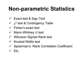
Non-parametric Statistics Exact test & Sign Test  2 test & Contingency Table Fisher’s exact test Mann-Whitney U test Wilcoxon Signed Rank test Kruskal -Wallis test Spearman’s Rank Correlation Coefficient Etc.

Why do we use nonparametric tests? Parametric tests are robust and versatile; are versatile to tests two or more variable & their interactions; use in several experimental designs;

Why do we use nonparametric tests? Parametric tests can’t use when data are extreme violation of assumptions; is inappropriate if scaling of data is not properly made so. can’t use when data are extreme violation of assumptions; Skewed data or data are not in normal distribution is inappropriate if scaling of data is not properly made so. Data are measured in nominal or rank scales

Exact test for Goodness of Fit ONE nominal variable Two or more mutually exclusive categories small N (  1,000) and independent observations Hypotheses Ho : The observed data in each category is equal to that predicted by biological theory H1 : The observed data in each category differs from that the expected Example – sex ratio as 1:1 or phenotypes ratio as 3:1

Exact test for Goodness of Fit Probability is directly calculated from the observed data under null hypothesis For binomial experiment, i.e. only 2 categories, the probability Y of k successes in n trials is obtained:   k = numbers of successes n = total number of trials p = the expected proportion of successes if Ho is true

Exact test for Goodness of Fit In Excel 2010+, Y can be calculated as: =BINOM.DIST( k,n,p,FALSE ) However, to test hypothesis, the probability P must include not only as extreme case as in observed data but also more extreme cases than in observed data; that is P = BINOM.DIST(k,n,p,TRUE)P from this function is the sum of Y for k, k-1, …, 0 successes and this P is an one-tailed PIf p is 0.5, the two-tailed P is 2(one-tailed P)

Exact test for Goodness of Fit A researcher wants to know if his cat use both paws (left & right ones) equally. A cat is irritated by a ribbon, and numbers of a left paws and a right paws used to catch a ribbon are counted The result is that a ribbon were caught 8 times by a right paw and only 2 by a left one Hypotheses Ho : A cat equally uses both paws H1 : A cat does not equally uses both paws Replace k =2, p =0.5, n=10 into BINOM.DIST(k,n,p,TRUE) yielded P = 0.055 for using a left paw 2, 1, 0 timesIf we consider the other extreme as well, i.e. using a right paws 2, 1, 0 times, it gives P = 0.110. Thus, accept Ho

Exact test for Goodness of Fit If p  0.5, two-tailed P must be calculated by another approaches A researcher knows that his cats are heterozygous at a hair-length gene, and the short-hair is dominant allele. So she expects to get short-hair kitten 75% and long-hair kittens 25% after crossing them The result is that she got 7 short-hair kittens and 5 long-hair kittens Hypotheses Ho : The ratio of short-hair kitten to long-hair kittens is 3 to 1H1 : The ratio of short-hair kitten to long-hair kittens is not 3 to 1SPSS calculates P by the “method of small P values”How, manually?

Exact test for Goodness of Fit p=0.75 for short-hair allele #kittens, k , for n =12 p=0.25 for long-hair allele P values for k P values for k 0.0000000596 0 0.0316763520 0.0000021458 1 0.12670540810.000035405220.23229324820.000354051630.25810360910.002389848240.19357770680.011471271550.10324144360.040149450360.04014945030.103241443670.01147127150.193577706880.00238984820.258103609190.00035405160.2322932482100.00003540520.1267054081110.00000214580.0316763520120.0000000596 0.157643676 0.031676352 0.157643676 0.031676352 P = 0.189320028, thus accept Ho = BINOM.DIST( k,n,p,FALSE )

Multinomial exact test for goodness-of-fit test Flower phenotypes from genetic cross in which the expect outcome of a 9:3:3:1 ratio of purple, red, blue, and white You get 72 purple , 38 red , 20 blue , and 18 white Analyzed in SPSS, you get a sig. of 0.0016  reject Ho: ratio of genetic cross is 9:3:3:1, then accept H1: ratio of genetic cross is NOT 9:3:3:1Next puzzles: which phenotype(s) is deviated from the expectation?Do Post-hoc test by conducting binomial exact tests for each category vs. the sum of all others categories with Bonferroni-correction significance level

Post-hoc test for multinomial exact test for goodness-of-fit test eg . Reject Ho: a ratio of purple, red, blue, and white is 9:3:3:1 Four tests Ho: purple : others is a ratio of 9:7 Ho: red : others is a ratio of 3:13 Ho: blue : others is a ratio of 3:13Ho: white : others is a ratio of 1:15Sig. for four testsSig. = 0.068Sig. = 0.035Sig. = 0.114Sig. = 0.005Bonferroni correction significant level for =0.05 is Only test#4 has Sig. < 0.0125  white is deviated from expected, i.e. more white than expected (18:130 ≈ 1:7.2)  

2 test – Goodness of Fit test ONE nominal variable; two or more mutually exclusive categories, large N (>1000), and independent observations Example: number of individuals with genotype TT , Tt , or tt those with pollen phenotype round and elliptic.Calculation: O i = observed value in category i E i = expected value in category i

2 test – Goodness of Fit test The shape of  2 distribution depending on degree of freedom Extrinsic null hypothesis : The predicted proportions are known from the null hypothesis before collecting data. The degree of freedom ( d.f. ) = n-1, where n is number of categories in a variableExample:- Sex ratio of male:female = 1:1, d.f. = 2-1 = 1 Reject Ho if 2cal  2crit

2 test – Goodness of Fit test The shape of  2 distribution depending on degree of freedom Intrinsic null hypothesis : One or more parameters are estimated from the data in order to get the values for the null hypothesis. The degree of freedom d.f. = n-parameter(s)-1 Ex. Genotypes of a codominant gene: LL, LS & SS, d.f. = 3-1-1 = 1Reject Ho if 2cal  2crit

Accept / Reject Ho

Example: Extrinsic null hypothesis TT Tt tt Observed 42 110 48 Expected H 0 : Ratio of genotypes TT : Tt : tt = 1:2:1 H 1 : Ratio of genotypes TT : Tt : tt ≠ 1:2:1 Total = 42 + 110 + 48 = 200 Ratio = 1 + 2 + 1 = 4 Thus, 1 part = 200  4 = 50

Example: Extrinsic null hypothesis TT Tt tt Total Observed 42 110 48 200 Expected 50 100 50 200 differences -8 10 -2  2 64 100 42crit = 5.991, df = 2,  = 0.05. Thus, ACCEPT Ho. 

Example: Intrinsic null hypothesis LL LS SS Observed 14 21 25 Expected H 0 : Population is in Hardy-Weinberg equilibrium H 1 : Population is not in Hardy-Weinberg equilibrium p + q = 1 p 2 + 2pg + q 2 = 1

Example: Intrinsic null hypothesis Allele frequencies ( for diploid): Total alleles = ( 14 + 21 + 25) 2 = 120 Thus, genotype frequencies is 0.167 LL , 0.483 LS , 0.350 SS Total = 14 + 21 + 25 = 60  LL = 0.167  60 = 10.02 LS = 0.483  60 = 28.98 SS = 0.350  60 = 21.00 

Example: Intrinsic null hypothesis LL LS SS Observed 14 21 25 Expected 10.02 28.98 21    2 crit = 3.841, df = 1,  = 0.05. Thus , REJECT Ho.

2 test for Contingency Table or R x C table Test of Homogeneity A test for the determination of whether or not the proportion are the same in two independent samples One set of marginal totals are fixed; the others are free to vary.

2 test for Contingency Table or R x C table Test of Independence or Test of association between/among variablesA test for the independence of two [or more] characteristics in the same sample when neither characteristic is particularly appropriate as a denominatorAll marginal totals are free to vary

Test of Homogeneity Age at first birth Status ≥30 ≤ 29 Total Case 683 2537 3,220 Control 1498 8747 10,245 Total 2,181 11,284 13,465 Variable A : Incidence of breast cancer Case : women with breast cancerControl : women without breast cancerVariable B: Age of women giving the first child≥30 : women with age at first birth ≥30≤29 : women with age at first birth ≤ 29Let p1 = the probability that age at first birth is ≥30 in CASE women with at least one birth p2 = the probability that age at first birth is ≥30 in CONTROL women with at least one birthThe problem is whether or not p1 = p2, or one want to test these hypotheses: Ho : p1 = p2 vs. H1 : p1 = p2

Test of Independence First food-frequency questionnaire Second food-frequency questionnaire High Normal Total High 15 5 20 Normal 9 21 30 Total 24 26 50 Question : Is there any relationship between the two reported measures of dietary cholesterol for the same person?

Variable B Variable A 1 2 3 … c 1 n 11 n 12 n 13 … n 1c n 1  2 n 21 n22n23…n2cn2:………………rnr1 n r2 n r3 … n rc n r  n  1 n  2 n  3 … n  c n Where n = total number of samples n ij = observed numbers in ( ij) th cell n i  = marginal total in i th row , I = 1, …, r n j = marginal total in j th column j = 1, …, c Calculating of E ij : Reject H o if  2 cal   2 crit at df = (r-1)(c-1)

Example: Test of Homogeneity Age at first birth Status ≥30 ≤ 29 Case 683 2537 Control 1498 8747 Let p 1 = the probability that age at first birth is ≥30 in CASE women with at least one birth p 2 = the probability that age at first birth is ≥30 in CONTROL women with at least one birth Ho : p1 = p2 vs. H1 : p1 = p2

Example: Test of Homogeneity Age at first birth Status ≥30 ≤ 29 Total Case 683 2537 3,220 Control 1498 8747 10,245 Total 2,181 11,284 13,465 Age at first birth Status ≥30≤29TotalCase3,220Control10,245Total2,18111,28413,4652cal = 78.37df = (2-1)(2-1) = 1p = 8.54 x 10⁻¹⁹2crit,  = 0.05 = 3.84p is function CHISQ.DIST.RT(2cal , df)

Experiencing flu Y N inoculated Y 150 200 N 300 250 900 Example: Test of Independence H0: Vaccine inoculation and flu susceptible are independent. H1: Vaccine inoculation and flu susceptible are NOT independent. Variable A : Experiencing flu? Yes No Variable B : Vaccinated Yes No

Experiencing flu Y N inoculated Y 150 175 200 175 350 N 300 275 250 275 550 450 450 900  2 cal = 11.68df = (2-1)(2-1) = 1p = 0.000632crit,  = 0.05 = 3.84

Pos-Hoc test for a table larger than 2x2 Method I : Calculating residual approach Calculate standardized residuals for each cell: More appropriately, adjusted standardized residuals should be used If absolute of adjusted standardized residuals are greater than 1.96  those cell are deviated from expected at sig. level of 0.05This is an uncorrected significance level as Method II : Partitioning approachAnalyze 2x2 subtables orthogonally partitioned from the original tableuse  2 tests with Bonferroni correction of the P valueAlternatives to Method IIConduct 2x2 tests for each category vs. the sum of all others categories with Bonferroni-correction significance level Conduct 2x2 test for each pair of categories with Bonferroni-correction significance level  

Criteria to partitioning approach(According to Agresti , A. (2013). Categorical data analysis (3rd ed.). Hoboken NJ: Wiley .) T he first rule is “The df for the subtables must sum to the df for the full table ”The second rule is “Each cell count in the full table must be a cell count in one and only one subtable” The third rule is “Each marginal total of the full table must be a marginal total for one and only one subtable” Finally, Agresti cautions that “for a certain partitioning, when the subtable df values sum properly but the G2 [Likelihood Ratio] values do not, the components are not independent”

Pos-Hoc test – Partitioning approach I II III A a b c B d e f C g h i I II III A a b c BdefCghiIIIIIIAabcBdefCghiIIIIIIAabcBdefCghiIIIIIIAabcBdefCghiPartitioning

Make sense?   Experiencing flu? Total Yes No Vaccine innoculation Yes Count 150 200 350 Expected Count 175.0 175.0 350.0 % within Vaccine innoculation 42.9% 57.1% 100.0% % within Experiencing flu? 33.3%44.4%38.9%Residual-25.025.0 Std. Residual-1.91.9 Adjusted Residual-3.43.4 NoCount300250550Expected Count275.0275.0550.0 % within Vaccine innoculation 54.5% 45.5% 100.0% % within Experiencing flu? 66.7% 55.6% 61.1% Residual 25.0 -25.0   Std. Residual 1.5 -1.5   Adjusted Residual 3.4 -3.4    

Example: 10 x 2 table Goiter test Positive Negative Bangkok 36 500 Chaingmai 17 350 Nan 12 300 Nakornsawan 1 300 Saraburi 4 350 Chonburi 14 500 Udonthani 7 200 Surin 27 500 Srisaket 2 200 Chumpon 4 200 H0: Proportion between positive goiter test in men in different province is the same H1: Proportion between positive goiter test in men in different province is not the same Variable A : Test result Positive negative Variable B : Location Bangkok Chiangmai …

Location observed expected Positive Negative Positive Negative Positive Negative Bangkok 36 464 18.23529 481.7647 17.30626 0.65506 Chaingmai 17 333 12.76471 337.2353 1.405259 0.053191 Nan1228810.94118289.05880.1024670.003878Nakornsawan 1 299 10.94118 289.0588 9.032574 0.341892 Saraburi 4 346 12.76471 337.2353 6.018162 0.227794 Chonburi 14 486 18.23529 481.7647 0.983681 0.037233 Udonthani 7 193 7.294118 192.7059 0.01186 0 0.000449 Surin 27 473 18.23529 481.7647 4.212713 0.159456 Srisaket 2 198 7.294118 192.7059 3.842505 0.145443 Chumpon 4 196 7.294118 192.7059 1.487666 0.05631 Location observed expected Positive Negative Positive Negative Positive Negative Bangkok 36 464 18.23529 481.7647 17.30626 0.65506 Chaingmai 17 333 12.76471 337.2353 1.405259 0.053191 Nan 12 288 10.94118 289.0588 0.102467 0.003878 Nakornsawan 1 299 10.94118 289.0588 9.032574 0.341892 Saraburi 4 346 12.76471 337.2353 6.018162 0.227794 Chonburi 14 486 18.23529 481.7647 0.983681 0.037233 Udonthani 7 1937.294118192.70590.0118600.000449Surin2747318.23529481.76474.2127130.159456Srisaket21987.294118192.70593.8425050.145443Chumpon41967.294118192.70591.4876660.05631 2cal = 46.08df = (10-1)(2-1) = 9p = 5.82 x 10⁻⁷  2 crit,  = 0.05 = 16.919

  Goiter test result Positive Negative Province Bangkok Count 36 464 Expected Count 18.2 481.8 Adjusted Residual 4.6 -4.6 Chaingmai Count 17 333 Expected Count 12.8 337.2 Adjusted Residual 1.3-1.3NanCount12288Expected Count10.9289.1Adjusted Residual.3-.3NakornsawanCount1299Expected Count10.9289.1Adjusted Residual-3.2 3.2 Saraburi Count 4 346 Expected Count 12.8 337.2 Adjusted Residual -2.6 2.6 Chonburi Count 14 486 Expected Count 18.2 481.8 Adjusted Residual -1.1 1.1 Udonthani Count 7 193 Expected Count 7.3 192.7 Adjusted Residual -.1 .1 Surin Count 27 473 Expected Count 18.2 481.8 Adjusted Residual 2.3 -2.3 Srisaket Count 2 198 Expected Count 7.3 192.7 Adjusted Residual -2.1 2.1 Chumpon Count 4 196 Expected Count 7.3 192.7 Adjusted Residual -1.3 1.3  

Tests of 2x2 subtablesone category vs. all others Location observed Positive Negative p-value Bangkok 36 464 0.000004 all others 88 2812 Chaingmai 17 333 0.202283 all others 107 2943 Nan 12 288 0.732711all others1122988Nakornsawan12990.001344all others1232977Saraburi43460.008323all others1202930LocationobservedPositiveNegativep-valueChonburi144860.273935all others1102790Udonthani71930.908954all others1173083Surin 27 473 0.023570 all others 97 2803 Srisaket 2 198 0.039547 all others 122 3078 Chumpon 4 196 0.200260 all others 120 3080  

Test of 2x2 subtables: two categories No disease Coronary artery disease ins/ins 268 807 ins/del 199 759 del/del 42 184 No disease Coronary artery disease ins/ins 268 807 ins/del 199 759 No disease Coronary artery disease ins/ins 268807del/del42184No diseaseCoronary artery diseaseins/del199759del/del421842=7.26, df=2, p=0.0272=4.95, df=1, p=0.0272=4.14, df=1, p=0.0422=0.54, df=1, p=0.4617 

Alternative to  2 test for RxC table: Fisher’s exact test A 2  2 contingency table (but can be applied to any m  n table)Expected values in any cell is less than 5 members of two independent groups can fall into one of two mutually exclusive categories. The test is used to determine whether the proportions of those falling into each category differs by groupsOne- or two-tail exact probabilities can be calculated

How to calculate Fisher’s p-value C 1 C 2 R 1 A B A+B R 2 C D C+D A+C B+D N In order to calculate the significance of the observed data, i.e. the total probability of observing data as extreme or more extreme if the null hypothesis is true, we have to calculate the values of p for both these tables, and add them together.

Example: Fisher’s p-value Men Women Dieting 1 9 10 Not dieting 11 3 14 12 12 24 Fisher showed that we could deal only with cases where the marginal totals are the same as in the observed table . Thus, there are 11 cases; one extreme data is here! In order to calculate the significance of the observed data, i.e. the total probability of observing data as extreme or more extreme if the null hypothesis is true, we have to calculate the values of p for both these tables, and add them together. Men WomenDieting01010Not dieting1221412 12 24 Observed data Extreme data

Example: More Fisher’s p-value 2 3 6 4 1 4 7 3 4 1 4 6 3 2 5 5 5 0 3 7 0 5 820.007 0.093 0.326 0.392 0.163 0.019 One-tail p = 0.007+0.093+0.326 = 0.426 Two-tail p = 0.007+0.093+0.326 + 0.163 +0.019 = 0.608

Example: Fisher’s p-value Cured Sicked Antibiotic treatment 4 9 13 Fecal transfer 13 3 16 17 12 29 Fisher showed that we could deal only with cases where the marginal totals are the same as in the observed table . Thus, there are 11 cases; one extreme data is here! In order to calculate the significance of the observed data, i.e. the total probability of observing data as extreme or more extreme if the null hypothesis is true, we have to calculate the values of p for both these tables, and add them together. Cured SickedAntibiotic treatment11213Fecal transfer1601617 12 29 Observed data Extreme data

Example: Fisher’s p-values 9 4 0.177317 8 8 8 5 0.283708 9 7 7 6 0.264794 10 6 6 7 0.144433 11 5 5 8 0.045135124490.0077151333100.00066114 2 2 11 0.000024 15 1 1 12 0.000000 16 0 13 0 0.000035 4 12 12 1 0.001094 5 11 11 2 0.012036 6 10 10 3 0.063046 7 9 One-tail p = 0.007715+[0.000661+0. 000024+0.000000] = 0.008401 Two-tail p = [ 0.007715+0.000661+0.000024+0.000000]+[0.001094+0.000035] = 0.009530

Testing your mind Suppose that we have a population of fungal spores which clearly fall into two size categories, large and small. We incubate these spores on agar and count the number of spores that germinate by producing a single outgrowth or multiple outgrowths . Spores counted : 120 large spores, of which 80 form multiple outgrowths and 40 produce single outgrowths 60 small spores, of which 18 form multiple outgrowths and 42 produce single outgrowths You want to know if there is any difference between two classes of spores, what test you should carry out? Why? What hypothesis to set up? How to do the test?

Another one… In order to test if these two genes are independently segregated, phenotypes in F2 generation were scored. The expected frequencies if genes being independently segregated should be 9:3:3:1 . Here is the result: Of 1,132 plants, 705 are tall with linear leaves, 145 are tall but broad leaves, 152 are stout with linear leaves, and 130 are stout with broad leaves. what test you should carry out? Why? What hypothesis to set up? How to do the test?

Another one… Two types of Vibrio botanicus strains have been suspected of causing diseases in squirrels. An experiment was conducted, and found that strain TSSciB54678 caused severe lesion in 9 out of 12 squirrels while strain TSSciB60125 caused mild lesion in 2 out of 20 squirrels. What kind of test should be carry out to indicate that these 2 strains causing diseases in different manner? Why? Are there any other test?