/
CS 240A:  Solving Ax = b in parallel CS 240A:  Solving Ax = b in parallel

CS 240A: Solving Ax = b in parallel - PowerPoint Presentation

celsa-spraggs
celsa-spraggs . @celsa-spraggs
Follow
391 views
Uploaded On 2017-11-03

CS 240A: Solving Ax = b in parallel - PPT Presentation

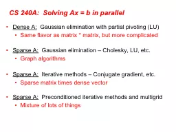
Dense A Gaussian elimination with partial pivoting LU Same flavor as matrix matrix but more complicated Sparse A Gaussian elimination Cholesky LU etc Graph algorithms Sparse A ID: 602072

matrix sparse graph solve sparse matrix solve graph methods iterative cholesky parallel gaussian elimination fill storage vector problem time

Share:

Link:

Embed:

Download Presentation from below link

Download Presentation The PPT/PDF document "CS 240A: Solving Ax = b in parallel" is the property of its rightful owner. Permission is granted to download and print the materials on this web site for personal, non-commercial use only, and to display it on your personal computer provided you do not modify the materials and that you retain all copyright notices contained in the materials. By downloading content from our website, you accept the terms of this agreement.


Presentation Transcript

Slide1

CS 240A: Solving Ax = b in parallel

Dense A:

Gaussian elimination with partial pivoting (LU)

Same flavor as matrix * matrix, but more complicated

Sparse A:

Gaussian elimination – Cholesky, LU, etc.

Graph algorithms

Sparse A:

Iterative methods – Conjugate gradient, etc.

Sparse matrix times dense vector

Sparse A:

Preconditioned iterative methods and multigrid

Mixture of lots of thingsSlide2

Matrix and Graph

Edge from row

i

to column j for nonzero A(i,j) No edges for diagonal nonzerosIf A is symmetric, G(A) is an undirected graph Symmetric permutation PAPT renumbers the vertices

1

2

3

4

7

6

5

A

G(A) Slide3

Compressed Sparse Matrix Storage

Full storage:

2-dimensional array.(nrows*ncols) memory.31

0

53

0

59

0

41

26

0

31

41

59

26

53

1

3

2

3

1

Sparse storage:

Compressed storage by columns

(CSC).

Three 1-dimensional arrays.

(2*nzs + ncols + 1) memory.

Similarly,

CSR.

1

3

5

6

value:

row:

colstart:Slide4

The Landscape of Ax=b Solvers

Direct

A = LU

Iterative

y

= Ay

Non-

symmetric

Symmetric

positive

definite

More Robust

Less Storage (if sparse)

More Robust

More GeneralSlide5

CS 240A: Solving Ax = b in parallel

Dense A: Gaussian elimination with partial pivoting (LU)

See April 15 slides

Same flavor as matrix * matrix, but more complicatedSparse A: Gaussian elimination – Cholesky, LU, etc.Graph algorithmsSparse A: Iterative methods – Conjugate gradient, etc.Sparse matrix times dense vectorSparse A: Preconditioned iterative methods and multigridMixture of lots of thingsSlide6

For a symmetric, positive definite matrix:

Matrix factorization

:

A = LLT (Cholesky factorization)Forward triangular solve: Ly =

b

Backward triangular solve: LT

x = y

For a nonsymmetric matrix:

Matrix factorization: PA = LU (Partial pivoting

). . .

Gaussian elimination to solve Ax = bSlide7

Sparse Column Cholesky Factorization

for

j = 1 : n

L(j:n, j) = A(j:n, j); for k < j with L(j, k) nonzero % sparse cmod(j,k) L(j:n, j) = L(j:n, j) – L(j, k) * L(j:n, k); end; % sparse cdiv(j)

L(j, j) = sqrt(L(j, j));

L(j+1:n, j) = L(j+1:n, j) / L(j, j);end;

Column j of A becomes column j of L

L

L

L

T

A

jSlide8

8

Irregular mesh: NASA Airfoil in 2DSlide9

Graphs and Sparse Matrices: Cholesky factorization

10

1

3

2

4

5

6

7

8

9

10

1

3

2

4

5

6

7

8

9

G(A)

G

+

(A)

[

chordal

]

Symmetric Gaussian elimination:

for j = 1 to n

add edges between j

s

higher-numbered neighbors

Fill

:

new

nonzeros

in factorSlide10

Permutations of the 2-D model problem

Theorem:

With the natural permutation, the n-vertex model problem has (n3/2) fill. (“order exactly”)Theorem:

With any permutation, the n-vertex model problem has

(n log n) fill. (“order at least

”)Theorem:

With a nested dissection permutation, the n-vertex model problem has O(n log n)

fill. (“order at most”)Slide11

Nested dissection ordering

A

separator in a graph G is a set S of vertices whose removal leaves at least two connected components.A nested dissection ordering for an n-vertex graph G numbers its vertices from 1 to n as follows:Find a separator S, whose removal leaves connected components T1, T2, …, T

kNumber the vertices of S from n-|S|+1 to n.

Recursively, number the vertices of each component:T1 from 1 to |T

1|, T2 from |T1

|+1 to |T1|+|T2|, etc.

If a component is small enough, number it arbitrarily.It all boils down to finding good separators!Slide12

Separators in theory

If

G

is a planar graph with n vertices, there exists a set of at most sqrt(6n) vertices whose removal leaves no connected component with more than 2n/3 vertices. (“Planar graphs have sqrt(n)-separators.”)

Well-shaped” finite element meshes in 3 dimensions have n2/3 -

separators. Also some other classes of graphs – trees, graphs of bounded genus, chordal graphs, bounded-excluded-minor graphs, …

Mostly these theorems come with efficient algorithms, but they aren’t used much.Slide13

Separators in practice

Graph partitioning heuristics have been an active research area for many years, often motivated by partitioning for parallel computation.

Some techniques:

Spectral partitioning (uses eigenvectors of Laplacian matrix of graph)Geometric partitioning (for meshes with specified vertex coordinates)Iterative-swapping (Kernighan-Lin, Fiduccia-Matheysses)Breadth-first search (fast but dated)Many popular modern codes (e.g. Metis, Chaco) use multilevel iterative swappingMatlab graph partitioning toolbox: see course web pageSlide14

Complexity of direct methods

n

1/2

n

1/3

2D

3D

Space (fill):

O(n log n)

O(n

4/3

)

Time (flops):

O(n

3/2

)

O(n

2

)

Time and space to solve any problem on any well-shaped finite element meshSlide15

CS 240A: Solving Ax = b in parallel

Dense A: Gaussian elimination with partial pivoting (LU)

See April 15 slides

Same flavor as matrix * matrix, but more complicatedSparse A: Gaussian elimination – Cholesky, LU, etc.Graph algorithmsSparse A: Iterative methods – Conjugate gradient, etc.Sparse matrix times dense vectorSparse A: Preconditioned iterative methods and multigridMixture of lots of thingsSlide16

The Landscape of Ax=b Solvers

Direct

A = LU

Iterative

y

= Ay

Non-

symmetric

Symmetric

positive

definite

More Robust

Less Storage (if sparse)

More Robust

More GeneralSlide17

Conjugate gradient iteration

One matrix-vector multiplication per iteration

Two vector dot products per iteration

Four n-vectors of working storagex0 = 0, r0 = b, d0

= r0

for k = 1, 2, 3, . . . α

k = (rTk-1r

k-1) / (dTk-1Adk-1

) step length xk

= xk-1 + αk d

k-1 approx solution rk

= rk-1 – αk Adk-1

residual β

k = (rTk rk

) / (rTk-1rk-1

) improvement d

k = rk + βk d

k-1 search directionSlide18

Sparse matrix data structure (stored by rows)

Full:

2-dimensional array of real or complex numbers(nrows*ncols) memory31

0

53

0

59

0

41

26

0

31

53

59

41

26

1

3

2

1

2

Sparse:

compressed row storage

about (2*nzs + nrows) memorySlide19

P

0

P

1

P

2

P

p-1

Each processor stores:

# of local nonzeros

range of local rows

nonzeros in CSR form

Distributed row sparse matrix data structureSlide20

Lay out matrix and vectors by rows

y(i) = sum(A(i,j)*x(j))

Skip terms with

A(i,j) = 0AlgorithmEach processor i: Broadcast x(i) Compute y(i) = A(i,:)*xOptimizations: reduce communication byOnly send as much of x as necessary to each proc Reorder matrix for better locality by graph partitioning

x

y

P0

P1

P2

P3

P0 P1 P2 P3

Matrix-vector product: Parallel implementationSlide21

Sparse Matrix-Vector MultiplicationSlide22

CS 240A: Solving Ax = b in parallel

Dense A: Gaussian elimination with partial pivoting (LU)

See April 15 slides

Same flavor as matrix * matrix, but more complicatedSparse A: Gaussian elimination – Cholesky, LU, etc.Graph algorithmsSparse A: Iterative methods – Conjugate gradient, etc.Sparse matrix times dense vectorSparse A: Preconditioned iterative methods and multigridMixture of lots of thingsSlide23

Conjugate gradient: Convergence

In exact arithmetic, CG converges in n steps

(completely unrealistic!!)Accuracy after k steps of CG is related to:consider polynomials of degree k that are equal to 1 at 0.how small can such a polynomial be at all the eigenvalues of A?Thus, eigenvalues close together are good.

Condition number:

κ(A) = ||A||2 ||A-1

||2 = λmax(A) / λ

min(A)Residual is reduced by a constant factor by

O( sqrt(κ(A)) ) iterations of CG.Slide24

Preconditioners

Suppose you had a matrix B such that:

condition number

κ(B-1A) is smallBy = z is easy to solveThen you could solve (B-1A)x = B

-1

b instead of Ax = bEach iteration of CG multiplies a vector by B-1

A:First multiply by AThen solve a system with BSlide25

Preconditioned conjugate gradient iteration

x

0

= 0, r0 = b, d0 = B-1 r0, y

0 = B

-1 r0

for k = 1, 2, 3, . . . αk

= (yTk-1rk-1

) / (dTk-1Adk-1)

step length xk = x

k-1 + αk dk-1 approx solution

rk = r

k-1 – αk Adk-1

residual yk = B

-1 rk

preconditioning solve βk

= (yTk rk) / (y

Tk-1rk-1)

improvement dk = y

k + βk dk-1

search direction

One matrix-vector multiplication per iterationOne solve with preconditioner per iterationSlide26

Choosing a good preconditioner

Suppose you had a matrix B such that:

condition number

κ(B-1A) is smallBy = z is easy to solveThen you could solve (B

-1A)x = B

-1b instead of Ax = bB = A is great for (1), not for (2)

B = I is great for (2), not for (1)Domain-specific approximations sometimes workB = diagonal of A sometimes works

Better: blend in some direct-methods ideas. . . Slide27

Incomplete Cholesky factorization (IC, ILU)

Compute factors of A by Gaussian elimination,

but ignore fill

Preconditioner B = RTR  A, not formed explicitlyCompute B-1z by triangular solves (in time nnz(A))

Total storage is O(nnz(A)), static data structure

Either symmetric (IC) or nonsymmetric (ILU)

x

A

R

T

RSlide28

Incomplete Cholesky and ILU: Variants

Allow one or more

levels of fill”unpredictable storage requirementsAllow fill whose magnitude exceeds a “drop tolerance”may get better approximate factors than levels of fillunpredictable storage requirements

choice of tolerance is ad hoc

Partial pivoting (for nonsymmetric A)“Modified ILU”

(MIC): Add dropped fill to diagonal of U or RA and RTR have same row sums

good in some PDE contexts

2

3

1

4

2

3

1

4Slide29

Incomplete Cholesky and ILU: Issues

Choice of parameters

good:

smooth transition from iterative to direct methodsbad: very ad hoc, problem-dependenttradeoff: time per iteration (more fill => more time) vs # of iterations (more fill => fewer iters)Effectiveness

condition number usually improves (only) by constant factor (except MIC for some problems from PDEs)

still, often good when tuned for a particular class of problemsParallelismTriangular solves are not very parallel

Reordering for parallel triangular solve by graph coloringSlide30

Coloring for parallel nonsymmetric preconditioning

[Aggarwal, Gibou, G]

Level set method for multiphase

interface problems in 3D

Nonsymmetric-structure,

second-order-accurate octree discretization.

BiCGSTAB preconditioned by parallel triangular solves.

263 million DOFSlide31

Sparse approximate inverses

Compute

B

-1  A explicitlyMinimize || B-1

A – I ||F

(in parallel, by columns)Variants: factored form of B

-1, more fill, . . Good: very parallel

Bad: effectiveness varies widely

A

B

-1Slide32

Other Krylov subspace methods

Nonsymmetric linear systems:

GMRES:

for i = 1, 2, 3, . . . find xi  Ki (A, b) such that ri

= (Axi

– b)  Ki (A, b)

But, no short recurrence => save old vectors => lots more space (Usually “restarted

” every k iterations to use less space.)BiCGStab, QMR, etc.:

Two spaces Ki (A, b) and K

i (AT, b)

w/ mutually orthogonal basesShort recurrences => O(n) space, but less robustConvergence and preconditioning more delicate than CG

Active area of current researchEigenvalues: Lanczos (symmetric),

Arnoldi (nonsymmetric)Slide33

Multigrid

For a PDE on a fine mesh, precondition using a solution on a coarser mesh

Use idea recursively on hierarchy of meshes

Solves the model problem (Poisson’s eqn) in linear time!Often useful when hierarchy of meshes can be builtHard to parallelize coarse meshes wellThis is just the intuition – lots of theory and technologySlide34

Complexity of linear solvers

2D

3D

Sparse Cholesky:

O(n

1.5

)

O(n

2

)

CG,

exact arithmetic:

O(n

2

)

O(n

2

)

CG,

no precond:

O(n

1.5

)

O(n

1.33

)

CG,

modified IC:

O(n

1.25

)

O(n

1.17

)

CG,

support trees:

O(n

1.20

) -> O(n

1+

)

O(n

1.75

) -> O(n1+ )

Multigrid:

O(n)

O(n)

n

1/2

n

1/3

Time to solve model problem (Poisson

s equation) on regular meshSlide35

Complexity of direct methods

n

1/2

n

1/3

2D

3D

Space (fill):

O(n log n)

O(n

4/3

)

Time (flops):

O(n

3/2

)

O(n

2

)

Time and space to solve any problem on any well-shaped finite element mesh