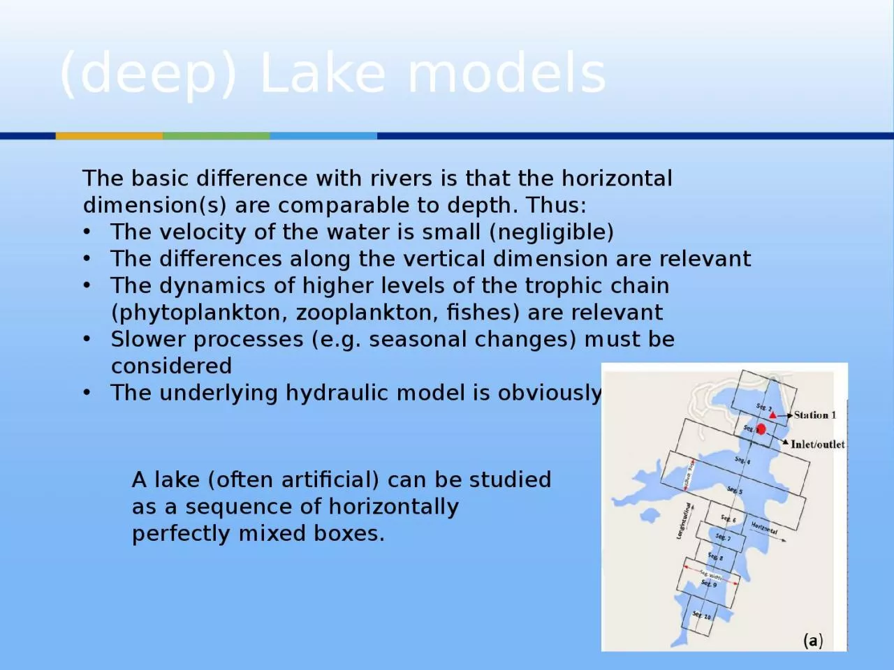
/
(deep ) Lake  models The basic difference with rivers is that the horizontal dimension(s) (deep ) Lake  models The basic difference with rivers is that the horizontal dimension(s)

(deep ) Lake models The basic difference with rivers is that the horizontal dimension(s) - PowerPoint Presentation

claire
claire . @claire
Follow
66 views
Uploaded On 2023-09-23

(deep ) Lake models The basic difference with rivers is that the horizontal dimension(s) - PPT Presentation

The velocity of the water is small negligible The differences along the vertical dimension are relevant The dynamics of higher levels of the trophic chain phytoplankton zooplankton fishes are relevant ID: 1019820

phytoplankton model input water model phytoplankton water input values temperature quality function rate output growth light random sensitivity control

Share:

Link:

Embed:

Download Presentation from below link

Download Presentation The PPT/PDF document "(deep ) Lake models The basic differenc..." is the property of its rightful owner. Permission is granted to download and print the materials on this web site for personal, non-commercial use only, and to display it on your personal computer provided you do not modify the materials and that you retain all copyright notices contained in the materials. By downloading content from our website, you accept the terms of this agreement.


Presentation Transcript

1. (deep) Lake modelsThe basic difference with rivers is that the horizontal dimension(s) are comparable to depth. Thus:The velocity of the water is small (negligible)The differences along the vertical dimension are relevantThe dynamics of higher levels of the trophic chain (phytoplankton, zooplankton, fishes) are relevantSlower processes (e.g. seasonal changes) must be consideredThe underlying hydraulic model is obviously different A lake (often artificial) can be studied as a sequence of horizontally perfectly mixed boxes.

2. LakesArtificialEx. Kariba Dam (Zambia-Zimbabwe) 128 m highNaturalEx. Miorina Dam, Lake Maggiore (Italy-Switzerland)3.3 m high

3. StratificationThe basic consequence of depth (in temperate climate) is water stratification.springwind heating faster than mixingsummersame temp. thus mixing warm water is less dense, thus floats, and needs lots of wind to mix

4. Stratification - 2Stratified lakes present three distinct zones. thermoclinedepth (m)temperature (°C)01030200103020region of rapid temperature changehypolimniumepilimniumsediments

5. Stratification - 3A typical yearly pattern in temperate countries (dimictic lakes  holomictic lakes)

6. Example 1: Lake Haag, OR, USA Surface area4.67 km2Average depth16 mMax. depth37 mWater volume73,900,000 m3

7. Example 2: Lake Pusiano, ItSurface area4.95 km2Average depth12.7 mMax. depth27 mCatchment area94.3 km2Water volume69,200,000 m3July temperature vs depth

8. EutrophicationNutrients feed phytoplankton causing its growthAbsense of circulation

9. Eutrophication consequencesLoss of water quality, fish death

10. Eutrophication processes (WASP7)PhytoplanktonNH3RespirationDis.Org. PDis.Org. NCBOD1CBOD2CBOD3PO4SSinorgSettlingPhotosynthesisDenitrificationNitrificationatmosphereDONO3AdsorptionOxidationMineralizationReaerationNNPCDetritusPeriphytonDeath&GazingPeriphyton is a mixture of algae, cyanobacteria, heterotrophic microbes attached to submerged surfaces

11. PhytoplanktonThe growth rate of a population of phytoplankton in a natural environment:is a complicated function of the species of phytoplankton present involves different reactions to solar radiation, temperature, and the balance between nutrient availability and phytoplankton requirementsDue to the lack of information to specify the growth kinetics for individual algal species all models characterizes the population as a whole by the total biomass of the phytoplankton present (measured in terms of chlorophyll concentration)

12. Phytoplankton - 2PhytNO3PO4NH3O C:N:PLightGrowth rate: Gmax = maximum specific growth rate constant at 20°C, 0.5 – 4.0 day-1 XT = temperature growth multiplier, dimensionless XL = light growth multiplier, dimensionless XN = nutrient growth multiplier, dimensionless

13. Phytoplankton growthwhere: G = temperature correction factor for growth (1.0 – 1.1) T = water temperature, °CTemperature multiplierNutrient multiplierDefines a limiting factorKMN semisaturation constant

14. Phytoplankton growth - 2XL depends on the light l(z) available for photosynthesis at depth z. It may be written using Michaelis-Menten formulationor Steele (1965) formulation where ls represents an optimal (maximum) light intensity.ButThe incident light on a water surface varies during the day and the seasonThe light intensity naturally decreases with depthThe presence of phytoplankton further increases light attenuation (self-shadowing)

15. Light attenuationThe light intensity dependence on depth l(z) can be expressed by the Beer-Lambert lawwhere l0 is the incident radiation on the surface and the functioncan be written as a polynomial function of phytoplankton concentration.

16. Typical seasonal patternsThe relation between phytoplankton and zooplankton is a typical predator-prey system.Algal blooms occur in spring.

17. Death rate:k1R = endogenous respiration rate constant, day-11R = temperature correction factor, dimensionlessk1D = mortality rate constant, day-1k1G = grazing rate constant, day-1, or m3/gZ-day if Z(t) specifiedZ(t) = zooplankton biomass time function, gZ/m3 (defaults to 1.0)Other components of phyoplankton dynamicsSettling rate:vS = settling velocity, m/dayAS = surface area, m2 V = segment volume, m3

18. Phosphorus cyclePhytoplanktonPO4Org. PDetr. PPhytoplankton PDetrital PGrowthDeathSettlingSettlingDeathDissolutionSettlingMineralizationGrowthDeathMineralizationDissolutionInorganic PDissolved organic P

19. Very high number of parametersDifficult to calibrate for a specific situation.Ex. Phosphorus cycle parameters

20. Fully distributed modelIt is necessary to compute all the internal processes for each volume in a grid and model the dispersion exchanges with the surrounding volumes (thousands of state variables)

21. Control of eutrophicationReduce loads (less detergents or fertilizers, better treatment,…)Artificial mixing Selective dischargesArtificial aeration

22. Defining the planning/control problemWater quality WQ is, in principle, a function of all the water components c1,…, cn in each location z1,z2,z3 and at any time instant t.In practice, we are not able to define the form of such a function.We thus define suitable indicators WQi for each components based on some kind of aggregation in time and/or space.where Stat() indicates some statistics over the spatial region Z and the time interval T.Examples:Summer average oxygen concentration in the hypolimniumYearly average of phytoplankton concentration in the upper 10 mNumber of times in a year in which the nitrogen concentration in the upper 1 m exceeds N.

23. Defining the planning/control problem - 2Additionally, we can assume that the overall water quality is some aggregation of the WQi . A common definition of the aggregation is an index formulated as a weighted sum:where the weights ai express some (subjective) measure of the importance of each factor in the assessment of water quality.The planning/control problem can be written: orwhere u are the decisions and Cost(u) their cost.

24. Defining the planning/control problem - 3As already noted (see slides on DPSIR), when used for planning/control, the model works in conditions different from those used for calibration/validation.The accuracy of the model cannot be proved.The model can thus be used to test the effect of an input (decision, parameter, boundary condition) on the output, to understand:the sense of the interaction (positive, negative)the entity of the interaction (larger, smaller than other input variables).To perform such Sensitivity/Uncertainty analysis, Monte Carlo simulation is normally used:Generate random numbers for model inputsRun the model with the randomized inputsStore the random input values and the corresponding model outputsRepeat a (high) number of times the steps (1-3)Calculate some output statistics (e.g. correlations between model outputs and random inputs)

25. Sensitivity/Uncertainty analysis- Define the input to be tested- Select a suitable distribution of values (normal, lognormal,…)- Generate a set of random values- Run the model- Store the results for the selected output- Analyse the output distribution- Compute the correlation I/O

26. Ex. YASAIw (US EPA)YASAIw is a free open-source framework for Monte Carlo simulation in Excel.Three main functions:1) To generate random model input values from a normal distribution:= GENNORMAL(mean, stdev)mean = nominal value for model input; stdev = e.g. 5% of mean for sensitivity analysis2) To save the random input values and use them in a sensitivity analysis:= SIMOUTPUT(x, name, code)x = cell address of the random inputname = unique name for the inputcode = 1 for input “assumption”3) To save the model output values and use them in a sensitivity analysis:= VBAOUTPUT(x, name, code)x = cell address of the model outputname = unique name for the outputcode = 2 for output “forecast”

27. Sensitivity analysis of QUAL2KwYASAIw GENNORMAL functions

28. YASAIw SIMOUTPUT functions

29. Links to the model output sheets

30.

31. Sensitivity average periphyton chlorophyll-ato the most sensitive model inputsSpearman's rank correlation coefficient (Spearman's rho), is a nonparametric measure of statistical dependence between two variables. It assesses how well the relationship between two variables can be described using a monotonic function.

32. An alternative approachThe solution of the planning/control problems requires the use of models to determine the link between decisions and water quality. However, a full quality model may not be necessary, since we are just interested in computing the link between decision and the defined water quality index.Develop a SURROGATE MODEL, i.e. a (simplified) model able to reproduce the required function, at least for a certain range of values of u, which means to substitute the original function WQ(u) with an approximation WQ=fs(u).

33. An alternative approach - 2The overall procedure is thus:Define the range of uDefine a structure for fsSimulate the original modelCalibrate the parameters of fsValidate fs Use fs in the optimization procedure Common forms for fs:A linear/polynomial functionA response surface A neural network…..It must be simple

34. The surrogate modelThe surrogate model:It’s NOT a copy of the systemIt’s based on the original model input and output and thus does not reproduce biochemical and physical phenomenaIt works correctly (the approximation is acceptable) only for the set of other input used for the original model simulation (design of experiments)It works correctly only within the range of u for what it has been calibratedIt’s faster to execute and thus can be repeated a high number of times within the optimization procedure

35. Surrogate modelling applicationDetermination of the «best» number and position of artificial aerators for an Australian artificial reservoir.suggested

36. Summary examplesSuppose you have to plan for the development of the agricultural activities along the Atbara river (Sudan):It is evident the this will impact on the water quality downstream, that must be maintained within reasonable values.Imagine you have a unlimited budget (unrealistic) for measurements, but no models is available.Determine the set of measurement necessary to calibrate a model that may be used to define the plan.

37. Water quality data will certainly represent different flow and temperature regimes.Even adopting a simple St-P model, we need to express the parameter values as a function of temperature T and flow Q.Thus, for instance,k1 (degradation)= k1(T,Q) = p1 p2(T-20) + p3 Qp4 k2 (reaeration)= k2(T,Q) = p5 Qp6 p7(T-20)The parameters to be estimated (assuming they are constant along each river reach) are 7 > 2. We need a at least 70-100 values + validation for every reach.