/
Graphics Volume 18, Number 3 July 1984 Graphics Volume 18, Number 3 July 1984

Graphics Volume 18, Number 3 July 1984 - PDF document

danika-pritchard
danika-pritchard . @danika-pritchard
Follow
419 views
Uploaded On 2015-11-18

Graphics Volume 18, Number 3 July 1984 - PPT Presentation

Ray Tracing L Cook Thomas Porter Loren Carpenter Division Lucasfilm Ltd tracing is one of the most elegant techniques in com puter graphics Many phenomena that are difficult or impossible with ot ID: 197187

Ray Tracing Cook Thomas

Share:

Link:

Embed:

Download Presentation from below link

Download Pdf The PPT/PDF document "Graphics Volume 18, Number 3 July 1984" is the property of its rightful owner. Permission is granted to download and print the materials on this web site for personal, non-commercial use only, and to display it on your personal computer provided you do not modify the materials and that you retain all copyright notices contained in the materials. By downloading content from our website, you accept the terms of this agreement.


Presentation Transcript

Graphics Volume 18, Number 3 July 1984 Ray Tracing L. Cook Thomas Porter Loren Carpenter Division Lucasfilm Ltd. tracing is one of the most elegant techniques in com- puter graphics. Many phenomena that are difficult or impossible with other techniques are simple with ray trac- ing, including shadows, reflections, and refracted light. Ray directions, however, have been determined precisely, and this has limited the capabilities of ray CATEGORIES AND SUBJECT DESCRIPTORS: ADDITIONAL KEY WORDS AND PHRASES: camera, constructive solid geometry, depth of field, focus, gloss, motion blur, penumbras, ray tracing, shadows, translucency, transparency Introduction tracing algorithms are elegant, simple, and powerful. They can render shadows, reflections, and refracted light, phenomena that are difficult or impossible with other techniquesIll. But ray tracing is currently limited to sharp shadows, sharp reflections, and sharp refraction. Permission to copy © 1984 ACM 0-89791-138-5/84/007/0137 $00.75 Ray traced images are sharp because ray directions are This approach has not been possible before because of aliasing. Ray tracing is a form of point Antialiasing opens up new possibilities ray tracing is a new approach to image syn- thesis. The key is that no extra rays are needed beyond those used for oversampling in space. For example, rather than taking multiple time samples at every spatial location, the rays are • Sampling the reflected ray according to the spec- ular distribution function produces gloss (blurred reflection). • Sampling the transmitted ray produces translu- cency (blurred transparency). • Sampling the solid angle of the light sources pro- duces penumbras. Sampling the camera lens area produces depth of field. • Sampling in time produces motion blur. 2. Shading The intensity I of the reflected light at a point on a sur- face is an integral over the hemisphere above the surface of an illumination function L and a reflection function R1. f f Oi)R(~i, Oi,~r, Or)d4bidOi (¢~.,0;) is the angle of incidence, and (¢~,0,) is the angle of reflection. The complexity of performing this integration has been avoided by making some simplifying assumptions. The following are some of these simplifications: • Assume that L is a 6 function, i.e., that L is zero except for light source directions and that the light sources can be treated as points. The integral is now replaced by a sum over certain discrete directions. This assumption causes sharp shadows. • Assume that all of the directions that are not light source directions can be grouped together into an ambient light source. This ambient light is the same in all directions, so that L is independent of ¢i and i may be removed from the integral. The integral of R may then be replaced by an average, or ambient, reflectance. • Assume that the reflectance function R is a 6 func- tion, i.e., that the surface is a mirror and reflects light only from the mirror direction. This assump- tion causes sharp reflections. A corresponding assumption for transmitted light causes sharp refrac- tion. The shading function may be too complex to compute analytically, but we can point sample its value by distri- buting the rays, thus avoiding these simplifying assump- tions. Illumination rays are not traced toward a single light direction, but are distributed according to the illumination function L. Reflected rays are not traced in a single mirror direction but are distributed according to the reflectance function R. 2.1. Gloss Reflections are mirror-like in computer graphics, but in real life reflections are often blurred or hazy. The dis- tinctness with which a surface reflects its environment is called reflections have been discussed by Whittedll and by Cook2. Any analytic simulation of these reflections must be based on the integral of the reflectance over some solid angle. Mirror reflections are determined by tracing rays from the surface in the mirror direction. Gloss can be calculated by distributing these secondary rays about the mirror direction. The distribution is weighted according to the same distribution function that determines the highlights. This method was originally suggested by Whitted11, and it replaces the usual specular component. Rays that reflect light sources produce highlights. 2.2. Translucency Light transmitted through an object is described by an equation similar to that for reflected light, except that the reflectance function R is replaced by a transmittance function T and the integral is performed over the hemi- sphere behind the surface. The transmitted light can have ambient, diffuse, and specular components5. Computer graphics has included transparency, in which T is assumed to be a 6 function and the images seen through transparent objects are sharp. Translucency differs from transparency in that the images seen through translucent objects are not distinct. The problem of translucency is analogous to the problem of gloss. Gloss requires an integral of the reflected light, and translu- cency requires a corresponding integral of the transmitted light. Translucency is calculated by distributing the secondary rays about the main direction of the transmitted light. Just as the distribution of the reflected rays is defined by the specular reflectance function, the distribution of the transmitted rays is defined by a specular transmittance function. 2.3. Penumbras Penumbras occur where a light source is partially obscured. The reflected intensity due to such a light is proportional to the solid angle of the visible portion of the light. The solid angle has been explicitly included in a shading model3, but no algorithms have been sug- gested for determining this solid angle because of the complexity of the computation involved. The only attempt at penumbras known to the authors seems to solve only a very special case7. Shadows can be calculated by tracing rays from the sur- face to the light sources, and penumbras can be calcu- lated by distributing these secondary rays. The shadow ray can be traced to any point on the light source, not just not to a single light source location. The distribu- tion of the shadow rays must be weighted according the projected area and brightness of different parts of the light source. The number of rays traced to each region should be proportional to the amount of the light's energy that would come from that region if the light was 138 Graphics Volume 18, Number 3 July 1984 D D ............ ---a.-............................ C image )lane lens focal plane Figure 1. Circle of Confusion. completely unobscured. The proportion of lighted sample points in a region of the surface is then equal to the pro- portion of that light's intensity that is visible in that region. Depth of Field and the eye have a finite lens aperture, and hence their images have a finite depth of field. Each point in the scene appears as a circle on the image plane. This circle is called the circle of confusion, and its size depends on the distance to the point and on the lens optics. Depth of field can be an unwanted artifact, but it can also be a desirable effect. Most computer graphics has been based on a pinhole camera model with every object in sharp focus. Potmesil simulated depth of field with a postprocessing technique. Each object is first rendered in sharp focus (i.e., with a pinhole camera model), and later each sharply rendered object is convolved with a filter the size of the circle of confusion8. The program spends most of its time in the focus postprocessor, and this time increases dramatically as the aperture decreases. Such a postprocessing approach can never be completely correct. This is because visibility is calculated from a sin- gle point, the center of tile lens. The view of the environ- ment is different from different parts of the lens, and the differences include changes in visibility and shading that cannot be accounted for by a postprocessing approach. For example, consider an object that is extremely out of focus in front of an object that is in focus. Visible sur- face calculations done with the pinhole model determine the visibility from the center of the lens. Because the front object is not in focus, parts of the focused object that are not visible from the center of the lens will be visible from other parts of the lens. Information about those parts will not available for the postprocessor, so the postprocessor cannot possibly get the correct result. There is another way to approach the depth of field prob- lem. Depth of field occurs because the lens is a finite size. Each point on the lens "looks" at the same point on the focal plane. The visible surfaces and the shading may be different as seen from different parts of the lens. The depth of field calculations should account for this and be an integral part of the visible surface and shading calcu- lations. Depth of field can be calculated by starting with the traditional ray from the center of the lens through point p on the focal plane. A point on the surface of the lens is selected and the ray from that point to p is traced. The camera specifications required for this calculation are the focal distance and the diameter of the lens F where F is n the focal length of the lens and n is the aperture number. This gives exactly the same circle of confusion as presented by Potmesil8. Because it integrates the depth of field calculations with the shading and visible surface calculations, this method gives a more accurate solution to the depth of field problem, with the exception that it does not account for diffraction effects. Figure 1 shows why this method gives the correct circle of confusion. The lens has a diameter of F and is n focused at a distance P so that the image plane is at a distance Vp, where = ~ for �PF. Points on the plane that is a distance D from the lens will focus at V D -~ ~ have a circle of confusion with diameter C of8 F C= IVD-V~I .v D For a point I on the image plane, the rays we trace lie inside the cone whose radius at D is F I P The image plane distance from a point on this cone to a point on the axis of the cone is r multiplied by the magnification of the lens. = r - ---~ . is easily shown that c' " Hence any points on the cone have a circle of confusion that just touches the image point /. Points outside the cone do not affect the image point and points inside the cone do. 4. Motion Blur Distributing the rays or sample points in time solves the motion blur problem. Before we discuss this method and how it works, let us first look in more detail at the motion blur problem and at previous attempts to solve it. The motion blur method described by Potmesil9 is not only expensive, it also separates the visible surface calcu- lation from the motion blur calculation. This is accept- able in some situations, but in most cases we cannot just calculate a still frame and blur the result. Some object entirely hidden in the still frame might be uncovered for part of the the time sampled by the blur. If we are to blur an object across a background, we have to know what the background is. Even if we know what the background is, there are prob- lems. For example, consider a biplane viewed from above, so that the lower wing is completely obscured by the upper wing. Because the upper wing is moving, the scenery below it would be seen through its blur, but unfortunately the lower wing would show through too. The lower wing should be hidden completely because it moves with the the upper wing and is obscured by it over the entire time interval. This particular problem can be solved by rendering the plane and background as separate elements, but not all pictures can easily be separated into elements. This solu- tion also does not allow for changes in visibility within a single object. This is particularly important for rotating objects. The situation is further complicated by the change in shading within a frame time. Consider a textured top spinning on a table. If we calculate only one shade per frame, the texture would be blurred properly, but unfortunately the highlights and shadows would be blurred too. On a real top, the highlights and shadows are not blurred at all by the spinning. They are blurred, of course, by any lateral motion of the top along the table or by the motion of a light source or the camera. The highlights should be blurred by the motion of the light and the camera, by the travel of the top along the table, and by the precession of the top, but not by the rotation of the top. Motion blurred shadows are also important and are not rendered correctly if we calculate only one shade per frame. Otherwise, for example, the blades of a fan could be motion blurred, but the shadows of those blades would strobe. All of this is simply to emphasize the tremendous com- plexity of the motion blur problem. The prospects for an analytic solution are dim. Such a solution would require solving the visible surface problem as a function of time as well as space. It would also involve integrating the texture and shading function of the visible surfaces over time. Point sampling seems to be the only approach that offers any promise of solving the motion blur problem. One point sampling solution was proposed by Korein and Badler6. Their method, however, point samples only in space, not in time. Changes in shading are not motion blurred. The method involves keeping a list of all objects that cross each sample point during the frame time, a list that could be quite long for a fast moving complex scene. They also impose the unfortunate restriction that both vertices of an edge must move at the same velocity. This creates holes in objects that change perspective severely during one frame, because the vertices move at drasti- cally different rates. Polygons with edges that share these vertices cannot remain adjoining. The algorithm is also limited to linear motion. If the motion is curved or if the vertices are allowed to move independently, the linear intersection equation becomes a higher order equa- tion. The resulting equation is expensive to solve and has multiple roots. Distributing the sample points in time solves the motion blur problem. The path of motion can be arbitrarily complex. The only requirement is the ability to calculate the position of the object at a specific time. Changes in visibility and shading are correctly accounted for. Sha- dows (umbras and penumbras), depth of field, reflections and intersections are all correctly motion blurred. By using different distributions of rays, the motion can be blurred with a box filter or a weighted filter or can be strobed. This distribution of the sample points in time does not involve adding any more sample points. Updating the object positions for each time is the only extra calculation needed for motion blur. Proper antialiasing is required or the picture will look strobed or have holes4. 140 Graphics Volume 18, Number 3 July 1984 Other Implications of the Algorithm surface calculation is straightforward. Since each ray occurs at a single instant of time, the first step is to update the positions of the objects for that instant of time. The next is to construct a ray from the lens the point and find the closest object that the ray intersects. Care must be taken in bounding moving" objects. The bound should depend on time so that of potentially visible objects does not grow unac- ceptably with their speed. Intersecting surfaces are handled trivially because we never have to calculate the line of intersection; we merely have to determine which is in front at a given location and time. At each sample point only one of the surfaces is visible. The intersections can even be motion blurred, a problem that would be terrifying with an analytic method. The union, intersection, difference problem is easily solved with ray tracing or point sampling10. These cal- culations are also correctly motion blurred. Transparency is easy even if the transparency is textured or varies with time. Let r be the transparency of a sur- face at the time and location it is pierced by the ray, and let R be the reflectance. R and r are wavelength depen- dent, and the color of the transparency is not necessarily the same as the color of the reflected light; for example, a red transparent plastic object may have a white highlight. If there are n-I transparent surfaces in front of the opaque surface, the light reaching the viewer is n-2 ~ + Rn-ll-Irl + " " " + + RI = ~ H ri. i=l i=l i~l i=l the surfaces form solid volumes, then each object has a r, and that r is scaled by the distance that the transmit- ted ray travels through that object. The motion blur and depth of field calculations work correctly for these tran- sparency calculations. The distributed approach can be adapted to a scanline algorithm as well as to ray tracing. The general motion blur and depth of field calculations have been incor- porated into a scanline algorithm using distributed sam- pling for the visible surface calculations. Special cases of penumbras, fuzzy reflections, and translucency have been successfully incorporated for fiat surfaces. Summary of the Algorithm intensity of a pixel on the screen is an analytic func- tion that involves several nested integrals: integrals over time, over the pixet region, and over the lens area, as well as an integral of reflectance times illumination over the reflected hemisphere and an integral of transmittance times illumination over the transmitted hemisphere. This integral can be tremendously complicated, but we can point sample the function regardless of how complicated it is. If the function depends on n parameters, the func- tion is sampled in the n dimensions defined by those parameters. Rather than adding more rays for each dimension, the existing rays are distributed in each dimension according to the values of the corresponding parameter. This summary of the distributed ray tracing algorithm is illustrated in Figure 2 for a single ray. • Choose a time for the ray and move the objects accordingly. The number of rays at a certain time is proportional to the value of the desired temporal filter at that time. 7 Light A Surface Lens Transmitted Ray Figure 2. Typical Distributed Ray Path on the toward the motion blurred green beveled the intersection faces is in in a 35 of focus, does the three on the an extended at any the paper and the Motion Blurred Balls in Graphics Volume 3 July 8 shows 5 billiard balls with motion blur and penumbras. Notice that the motion is not linear: the 9 ball changes direction abruptly in the middle of the frame, the 8 ball moves only during the middle of the frame, and the ,l ball only starts to move near the end of the frame. The shadows on the table are sharper where the balls are closer to the table; this most apparent in the stationary 1 ball. The reflections of the billiard balls and the room are motion blurred, as are the penumbras. Figures 3, 5, and 7 were rendered with a scanline adapta- tion of this algorithm. Figures 4, 6, and 8 were rendered with ray tracing. 8. Conclusions Distributed ray tracing a new paradigm for computer graphics which solves a number of hitherto unsolved or partially solved problems. The approach has also been successfully adapted to a scanline algorithm. It incor- porates depth of field calculations into the visible surface calculations, eliminating problems in previous methods. It makes possible blurred phenomena such as penumbras, gloss, and translucency. All of the above can be motion blurred by distributing the rays in time. These are not isolated solutions to isolated problems. This approach to image synthesis is practically no more expensive than standard ray tracing and solves all of these problems at once. The problems could not really be solved separately because they are all interrelated. Differences in shading, in penumbras, and in visibility are accounted for in the depth of field calculations. Changes in the depth of field and in visibility are motion blurred. The penumbra and shading calculations are motion blurred. All of these phenomena are related, and the new approach solves them all together by sampling the mul- tidimensional space they define. The key to this is the ability to antialias point sampling. References 1. COOK, ROBERT L., TURNER WHITTED, AND DONALD P. GREENBERG, Comprehensive Model for Image Synthesis. report 2. COOK, ROBERT L., "A Reflection Model for Realistic Image Synthesis," Master's thesis, Cornell Univer- sity, Ithaca, NY, December 1981. 3. COOK, ROBERT L. AND KENNETH E. TORRANCE, "A Reflection Model for Computer Graphics," Transactions on Graphics, 1, no. 1, pp. 7-24, January 1982. 4. COOK, ROBERT L., "Antialiased Point Sampling," Technical Memo #94, Lucasfilm Ltd, San Rafael, CA, October 3, 1983. 5. HUNTER, RICHARD S., Measurement of Appear- ance, Wiley & Sons, New York, 1975. 6. KOREIN, JONATHAN AND NORMAN BADLER, "Tem- poral Anti-Aliasing in Computer Generated Anima- tion," Graphics, 17, no. 3, pp. 377- 388, July 1983. 7. NISHITA, TOMOYUKI, ISAO OKAMURA, AND EIHACHIRO NAKAMAE, Art Show, 8. POTMESIL, MICHAEL AND INDRANIL CHAKRAVARTY, "Synthetic Image Generation with a Lens and Aper- ture Camera Model," Transactions on Graph- ics, 1, no. 2, pp. 85-108, April 1982. 9. POTMESIL, MICHAEL AND INDRANIL CtlAKRAVARTY, "Modeling Motion Blur in Computer-Generated Images," Graphics, 17, no. 3, pp. 389-399, July 1983. 10. ROTH, S. D., "Ray Casting for Modeling Solids," Graphics and Image Processing, 18, pp. 109-144, 1982. 11. WHITTED, TURNER, "An Improved Illumination Model for Shaded Display," of the ACM, 23, pp. 343-349, 1980. 9. Acknowledgements Rodney Stock proposed the approach to antialiased point sampling that formed the basis of the paradigm explored in this paper. John Lasseter drew the environment map of the pool hall for "1984". Ed Catmull worked with us in th~ image synthesis working group and helped develop and refine these ideas. He and Alvy Ray Smith provided invaluable suggestions along the way. Tom Duff wrote the ray tracing program that we adapted to distributed ray tracing. 144 Graphics Volume 3 July 8. 1984.