PDF-porous media Department of Environmental Sciences Riverside, CA, US

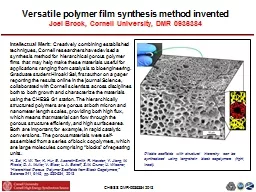
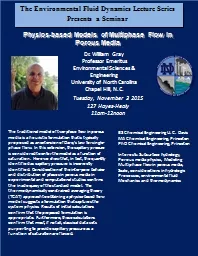
CEN Belgium EPORT OF THE Notes on HP1. & . Biomolecular. Engineering. University . of . Maryland. College Park, MD, 20742 . . 04/04/2013. Characterizing Porous Materials and Powders . Hao Wen. Prepared for defense practice talk. 3/29/2012. 2. Fuel cells - overview. Fuel cells convert . chemical. energy into . electricity. Applications varies from high temperature high power output to room temperature portable power sources.. ASEP MUHAMAD SAMSUDIN, S.T.,M.T.. MEMBRANE SEPARATION. MEMBRANE. Material . Source. Cross-section . Structure. Bulk . Structure. Geometry. Separation Regime. Organic/ Polymer. Inorganic. Symmetric. Asymmetric. Versatile . polymer film synthesis method . invented. Joel Brock, Cornell University, DMR 0936384. Pliable scaffolds with structural hierarchy can be synthesized using long-chain block . copolymers (right, inset).. OMICS Group International through its Open Access Initiative is committed to make genuine and reliable contributions to the scientific community. OMICS Group hosts over . 400. leading-edge peer reviewed Open Access Journals and organizes over . Series. Presents a Seminar. . Physics-based Models of Multiphase Flow in. Porous Media. The traditional model of two-phase flow in porous media is a heuristic formulation that is typically proposed as an extension of Darcy’s law for single-phase flow. In this extension, the capillary pressure is considered to enter the model as a function of saturation. Here we show that, in fact, the quantity identified as capillary pressure is incorrectly identified. Consideration of the inter-pore behavior and distribution of phases in porous media in experimental and computational studies confirms the inadequacy of the standard model. The thermodynamically constrained averaging theory (. and the . Mission Inn. Background image courtesy of the Library of Congress. Above. : Photograph of Main Street, Riverside, 1875. The future site of the Mission Inn is just out of frame, to the far right. . Non-vegetated GI and Effective Engineer-Contractor Communication. Presented to:. CWEA . Stormwater. Conference . Spring 2015 Seminar. Presented by:. April 17, 2015. Zack Knight, PE. Presentation Outline. HIGH DENSITY . TUNGSTEN BASE . POROUS . J. ETS. MEIR MAYSELESS & DOV . . IPS-15-7. 2. OUTLINE. INTRODUCTION. POWDERS. SIMULATIONS. CONCLUSIONS. 1. . The need to avoid plugging . in the . processing including filtration technology.. The Brinkman extension to Darcy’s law equation includes the effect of . wall. The introduction of 2. nd. order shear stress terms . ensures the variables like velocity and pressure to be continuous across the interface between . Department of Chemical & Biomolecular Engineering University of Maryland College Park, MD, 20742 04/04/2013 Characterizing Porous Materials and Powders 1 – Porous Pave® Background. In May 2016, APCC made a decision to install a relatively new asphaltalternative called “Porous Pave An application of acoat of the binder every threeyearswil May 13 2021seligibility to those 12 and older for COVID-19 vaccinationJuveniles under 18 will need to be accompanied by parent or legal guardian to get immunizationRiverside County health officials ar Lesson 5. Does the Bath Riverside development encourage sustainable communities?. Is Bath Riverside a sustainable community?. Active, inclusive and safe. Well run. Environmentally sensitive. Well designed and built.