/
Discrete Time and Discrete Event Modeling Formalisms and Th Discrete Time and Discrete Event Modeling Formalisms and Th

Discrete Time and Discrete Event Modeling Formalisms and Th - PowerPoint Presentation

debby-jeon
debby-jeon . @debby-jeon
Follow
492 views
Uploaded On 2016-04-22

Discrete Time and Discrete Event Modeling Formalisms and Th - PPT Presentation

Dr Feng Gu Way to study a system Cited from Simulation Modeling amp Analysis 3e by Law and Kelton 2000 p 4 Figure 11 Model taxonomy Modeling formalisms and their simulators Discrete time model and their simulators ID: 288536

discrete time event state time discrete state event model simulation cell automata cellular events life cells algorithm step scheduling

Share:

Link:

Embed:

Download Presentation from below link

Download Presentation The PPT/PDF document "Discrete Time and Discrete Event Modelin..." is the property of its rightful owner. Permission is granted to download and print the materials on this web site for personal, non-commercial use only, and to display it on your personal computer provided you do not modify the materials and that you retain all copyright notices contained in the materials. By downloading content from our website, you accept the terms of this agreement.


Presentation Transcript

Slide1

Discrete Time and Discrete Event Modeling Formalisms and Their Simulators

Dr. Feng GuSlide2

Way to study a system

Cited from Simulation, Modeling & Analysis (3/e) by Law and

Kelton, 2000, p. 4, Figure 1.1Slide3

Model taxonomySlide4

Modeling formalisms and their simulators

Discrete time model and their simulators

Differential equation models and their simulators

Discrete event models and their simulatorsSlide5

Discrete Time Models and Simulators

Discrete time models are usually the most intuitive to grasp all forms of dynamic models.

This formalism assumes a stepwise mode of execution.

At a particular time the model is in a particular state and it defines how its state changes. The next state usually depends on the current state and also what the environment’s influences currently are. Slide6

Discrete time model

Discrete time systems have numerous applications.

The most popular are in digital systems where the clock defines the discrete time steps.

It is also frequently used as approximations of continuous systems. To build a discrete time model, we have to define how the current state and the input from the environment determine the next state of the model. This can be done using a table.Slide7

Discrete time model

In discrete time models, time advances in discrete steps, which we assume are integer multiples of some basic period such as 1s, 1 day.

The transition/output table can also be described as follows: If the state at time t is q and the input at time t is x, then the state at time t+1 will be •(

q,x) and the output y at time t will be λ(q,x). Here • is called the state transition function and is the more abstract concept for the first three columns of the table. λ is called the output function. Slide8

Discrete time model

Question: specify •(

q,x

) and λ(q,x) for the table above •(q,x) = x λ(q,x) = xThe function •(q,x

) and λ(

q,x

) are more general than the table.

Now add time in the above specification.Slide9

Discrete time model

A sequent of state, q(0), q(1), q(2),… is called a

state trajectory. Having an arbitrary initial state q(0), subsequent states in the sequence are determined by

q(t+1) = •(q(t), x(t)) = x(t). Similarly, a corresponding output trajectory is given by y(t) = λ(q(t), x(t)) = x(t) .Question: write an algorithm to compute the state and output trajectories of a discrete time model given its input trajectory and its initial state.Slide10

Discrete time model

The following algorithm is an example of a simulator for a discrete time model:

Ti=0,

Tf=9 the starting and ending times, here 0 and 9 X(0) = 1, …, x(9) = 0 the input trajectory q(0) = 0 the initial state t=Ti While (t<=

T

f

){

y(t) =

λ(

q(t), x(t))

q(t+1) =

δ(

q(t), x(t))

t = t+1

}

Question: The computation complexity of this algorithm/Slide11

One-dimensional cell spaceSlide12

Cellular automata

A cellular automaton is an idealization of a physical phenomenon in which space and time are discredited and the state sets are discrete and finite.

Cellular automata have components, called cells, which are all identical with identical computational apparatus.

They are geometrically located on a one-, two-, or multidimensional grid and connected in a uniform way. The cells influencing a particular cell, called the neighborhood of the cell, are often chosen to be the cells located nearest in the geometrical sense. Time is also discrete, and the state of a cell at time t is a function of the states of a finite number of cells (called its neighborhood) at time t − 1. Each time the rules are applied to the whole grid a new generation is created.

Cellular automata were originally introduced by von Neumann and

Ulam

as idealization of biological self-production.Slide13

Example of CASlide14

One dimensional cellular automata

Below are tables defining the "rule 30 CA" and the "rule 110 CA" (in binary, 30 and 110 are written 11110 and 1101110, respectively) and graphical representations of them starting from a 1 in the center of each image:

Slide15

One dimensional cellular automata

Rule 110, like the Game of Life, exhibits what Wolfram calls class 4 behavior, which is neither completely random nor completely repetitive. Localized structures appear and interact in various complicated-looking ways. Slide16

One dimensional cellular automata

Rule 30 CA

http://modelingcommons.org/browse/one_model/1564#model_tabs_browse_applet

Rule 110 CAhttp://modelingcommons.org/browse/one_model/1562#model_tabs_browse_appletSlide17

Cellular automata

Wolfram systematically investigated all possible transition functions of one-dimensional cellular automata.

He found out that there exist four types of cellular automata that differ significantly in their behavior:

-Automata where any dynamic soon die out. -Automata that soon come to periodic behavior -Automata that show chaotic behavior -And the most interesting ones, automata whose behaviors are unpredictable and non-periodic but that showing interesting, regular patterns.Slide18

Class 1Slide19

Class 2Slide20

Class 3Slide21

Class 4Slide22

Game of life

Conway’s Game of Life is framed within a two-dimensional cell space structure

Each cell is in one of two possible states, live or dead. Every cell interacts with its eight neighbors, which are the cells that are directly horizontally, vertically, or diagonally adjacent. At each step in time, the following transitions occur:

-Any live cell with fewer than two live neighbors dies, as if by loneliness. -Any live cell with more than three live neighbors dies, as if by overcrowding. -Any live cell with two or three live neighbors lives, unchanged, to the next generation. -Any dead cell with exactly three live neighbors comes to life. Slide23

Game of life

http://en.wikipedia.org/wiki/Conway's_Game_of_Life

http://www.bitstorm.org/gameoflife http://math.com/students/wonders/life/life.htmlSlide24

Why is game of life interesting (http://math.com/students/wonders/life/life.html)

It is one of the simplest examples of what is sometimes called "emergent complexity" or "self-organizing systems."

It is the study of how elaborate patterns and behaviors can emerge from very simple rules. It helps us understand, for example, how the petals on a rose or the stripes on a zebra can arise from a tissue of living cells growing together. It can even help us understand the diversity of life that has evolved on earth.

In Life, as in nature, we observe many fascinating phenomena. Nature, however, is complicated and we aren't sure of all the rules. The game of Life lets us observe a system where we know all the rules. The rules described above are all that's needed to discover anything there is to know about Life, and we'll see that this includes a great deal. Unlike most computer games, the rules themselves create the patterns, rather than programmers creating a complex set of game situations.Slide25

Cellular automata simulation algorithm

How to develop a CA simulation algorithm?

The basic procedure for simulating a cellular automaton follows the discrete time simulation algorithm introduced earlier.

At every time step we scan all cells, applying the state transition function to each, and saving the next state in a second copy of the global state data structure. Then the clock advances to the next step. To do this we need to limit the space to a finite region. How to take care of the boundary cells? What is the computation complexity of this algorithm?Slide26

Discussion

Now consider an agent-based pedestrian crowd simulation. At each time step, each agent makes an decision of movement (based on its current state and its surrounding situation) and then carry out the movement. Slide27

DiscussionSlide28

Discussion

Now consider an agent-based pedestrian crowd simulation. At each time step, each agent makes an decision of movement (based on its current state and its surrounding situation) and then carry out the movement. Slide29

Cellular automata simulation algorithm

The basic procedure for simulating a cellular automaton follows the discrete time simulation algorithm introduced earlier.

At every time step we scan all cells, applying the state transition function to each, and saving the next state in a second copy of the global state data structure.

Then the clock advances to the next step. What is the computation complexity of this algorithm? A more efficient approach?Slide30

Discrete event approach to cellular automata simulation

In discrete time systems, at every time step each component undergoes a “state transition”; this occurs whether or not its state actually changes.

Often, only small number of components really change.

Define an event as a change in state (e.g.., births and deaths in the Game of Life). A discrete event simulation algorithm concentrates on processing events rather than cells and is inherently more efficient. How to design the algorithm?Slide31

Discrete event approach to cellular automata simulation

The basic idea is to try to predict whether a cell will possibly change state or will definitely be left unchanged in the next global state transition.

A cell will not change state at the next state transition time, if none of its neighboring cells changed state at the current state transition time.

Why?Slide32

Discrete event approach to cellular automata simulation

In a state transition mark those cells which actually changed state. From those, collect the cells that are their neighbors. The set collected contains all cells that can possibly change at the next step. All other cells will definitely be left unchanged.

Question: Analyze the computation complexity of this discrete event approach for cellular automata simulation.Slide33

Discrete event model

Discrete event models have many applications. Examples:

-Queue Model (Example: the service lines in a bank)

-Process workflow system such as manufactory system, supply chain -Control systems (Example: rail road dispatch control) -Ecological systems with the happenings of significant phenomenon (such as occurrence of a fire) -Computer networks (driven by arrival of packages or completion of tasks) -Any system where the concept of “change” is important even they are traditionally modeled by continuous models or discrete time models. (Example: decision making of a human being driven by changes in perception).

Discrete time model is a special case of discrete event model with each time step as an event.Slide34

A cellular automata with fitness

The original version of Game of Life assumes that all births and deaths take the same time (equal to a time step)

A more accurate representation assumes birth and death dependent on a quantity called fitness.

A cell attains positive fitness when its neighborhood is supportive, that is, when it has exactly 3 neighbors, and the fitness will diminish rapidly when its environment is hostile (<2 or >3 neighbors). Whenever the fitness reaches 0, the cell will die. A dead cell will have a negative fitness -2. When the environment is supportive and the fitness crosses the zero level, the cell will born. Assuming the fitness increase rate is 1 per second, decrease rate is -3 per second. A cell can have maximum fitness of 6.Slide35

An example

What is needed to model such a process?Slide36

Discussion

Discrete Time Modeling approach

-What are the q, x, y, delta function, and output function?

-(fitness should be part of q) Discrete Event Modeling approach -Consider one cell first -Then the whole cell spaceFor the discrete time model, what happens if the birth or death time is not integer? Slide37

Event-based approach

Concentrate on the interesting events only, namely births and deaths, as well as the changes in the neighborhood.

To do that, we need a means to determine when interesting things happen.

Events can be caused by the environment, such as the changes of the sum of alive neighbors. The occurrence of such external events are not under the control of the model component itself. On the other side, the component may schedule events to occur. Those are called internal events. Given a particular state, e.g., a particular fitness of the cell, a time advance is specified as the time it takes until the next internal event occurs, supposing that no external event happens in the meantime.Slide38

The exampleSlide39

Scheduling

How does time advance in a discrete time model and a discrete event model?

The concept of “scheduling” is central in discrete event modeling and simulation.

In a discrete time model, scheduling is implicit because the time advances in a fixed time step fashion. In a discrete event model, at any state, the model needs to explicitly schedule the next event. -Given a particular state, a time advance is specified as the time it takes until the next internal event occurs, supposing that no external event happens in the meantime. Slide40

Discrete event simulation

In discrete event simulation, one has to execute the scheduled internal events of the different cells at their event times.

Moreover, at any state change through an internal event we must take care to examine the cell’s neighbors for possible state changes.

A change in state may affect waiting times as well as result in scheduling of new events and cancellation of events. Slide41

Discrete event simulation

We see that the effect of a state transition may not only be to schedule new events, but also to cancel events that were scheduled in the past. (see from (a) to (b) in the figure)

Furthermore, see from (b) to (c) in the figure, the system can jump from the current time 1 to next event time 3. This illustrates efficiency advantage in discrete event simulation – during times when no events are scheduled, no components need to be scanned.

The situation at time 3 (Figure (b) also illustrates a problem in discrete event simulation – that of simultaneous events. Who goes first? -All simultaneous events undergo their state transitions together. -Define a priority among the components Slide42

Event scheduling

Event scheduling is a basic approach in discrete event simulation.

Because of its simplicity, event scheduling simulation is the preferred strategy when implementing customized simulation systems in procedural programming languages.

The event scheduling utilizes a event list, which stores a list of events that are ordered by increasing scheduling times. The event with earliest scheduled time is removed from the list and the clock is advanced to the time of this imminent event. The routine associated with the imminent event is executed. A tie-breaking procedure is employed if there is more than one such imminent events. Execution of the event routine may cause new events to be added in the proper place on the list. Also, existing events may be rescheduled or even canceled. The next cycle now begins with the clock advance to the earliest scheduled time.Slide43

Event schedulingSlide44

Event schedulingSlide45

Event list scheduling

Exercise: Hand execute the simulation algorithm for several cases: for example (1) inter-gen-time > service-time; (2) inter-gen-time = service-time; (3)inter-gen-time <service-time <2*inter-gen-timeSlide46

Discussion