/
RDF-3X: a RISC style Engine for RDF RDF-3X: a RISC style Engine for RDF

RDF-3X: a RISC style Engine for RDF - PowerPoint Presentation

ellena-manuel
ellena-manuel . @ellena-manuel
Follow
466 views
Uploaded On 2017-01-20

RDF-3X: a RISC style Engine for RDF - PPT Presentation

Ref Thomas Neumann and Gerhard Weikum PVLDB08 Presented by Pankaj Vanwari Course Advanced Databases CS 632 Motivation RDFResource Description Framework is schemafree structured information ID: 512092

query rdf triple data rdf query data triple indexes object sparql join selectivity graph joins storage triples index aggregated

Share:

Link:

Embed:

Download Presentation from below link

Download Presentation The PPT/PDF document "RDF-3X: a RISC style Engine for RDF" is the property of its rightful owner. Permission is granted to download and print the materials on this web site for personal, non-commercial use only, and to display it on your personal computer provided you do not modify the materials and that you retain all copyright notices contained in the materials. By downloading content from our website, you accept the terms of this agreement.


Presentation Transcript

Slide1

RDF-3X: a RISC style Engine for RDF

Ref: Thomas Neumann and Gerhard Weikum [PVLDB’08 ]

Presented by: Pankaj Vanwari

Course: Advanced Databases (CS 632)Slide2

Motivation

RDF(Resource Description Framework ) is schema-free structured information.

Increasingly popular in context of

Knowledge bases

Semantic Web

Life-Sciences and Online communities.

Managing large-scale RDF data includes challenges for

Storage layout, indexing and queryingSlide3

Overview

Introduction to RDF and SPARQL

Storage of RDF data

Query Translation and Processing

Query Optimization

Evaluation

Conclusion Slide4

Introduction to RDF

Standard model for data interchange on the Web.

Allows structured and semi-structured data to be mixed, exposed, and shared.

Conceptually a labeled graph

Linking structure forms a directed labeled graph where the edges represent the named link between two resources that are represented by the graph nodes.

Graph is stored as collection of facts. Each edge represents a fact (triple in RDF notation)

Triples have the form (subject; predicate; object)Slide5

RDF as labeled graph

Extends the linking structure of the Web by using URIs for relationship.

Subjects and predicates are identified by URI values.

Object can be another URI or a value (literal).Slide6

RDF Example: Conceptual View

id1

id11

id2

releaseYear

directedBy

hasTitle

roleName

hasCasting

actor

hasName

2008

Slumdog

Millionaire

Danny Boyle

Freida Pinto

id7

hasName

LatikaSlide7

RDF Eample

: Facts in triple form

(id1,

hasTitle

, "

Slumdog

Millionaire "),

(id1,

releaseYear

, "2009"),

(id1, directedBy,id7)

(id7,hasName,“Danny Boyle"),

(id1,

hasCasting

, id2),(id2, roleName, “

Latika"),(id2, actor, id11),(id11, hasName, " Freida Pinto"),and so on…RDF data is a (potentially huge) set of triples585 million triples – Size of data in Freebase120 million facts of 10 million entities in YAGO2Slide8

Introduction to SPARQL

SPARQL is used to query over RDF data.

Result can be result sets or RDF graphs.

SPARQL query for “The titles of all movies having

Freida

Pinto“ can be:

Select

?title

Where

{

?p

<

hasTitle

>

?title. ?p <hasCasting> ?s. ?s <actor> ?c. ?c<

hasName>“Freida Pinto“ }From the prevous example triples: ?c : id11 , ?s : id2, ?p : id1 and ?title : " Slumdog Millionaire "Slide9

SPARQL- Join graph

Each SPARQL query can be represented by a join graph. A possible join tree for the previous query:

Where P

1

= (

?p

<

hasTitle

>

?title

),

P

2

= (

?p <hasCasting>

?s), P3 = (?s <actor> ?c) and P4 =(?c <hasName> “Freida Pinto“ ) are triple patterns.Slide10

SPARQL: Query features

FROM clause to select a data set

PREFIX clause for Namespace Prefixes

WHERE clause supports

Star-shaped query

Long join path query

FILTER to restrict values by patterns/conditions

Union query

Optional query

For Result: ORDER BY, DISTINCT, CONSTRUCT, DESCRIBE and ASK clause Slide11

Problems in querying over RDF

RDF data storing, indexing and query processing is non-trivial:

Absence of global schema.

Very fine grained data items. instead of records or entities.

Execution plan optimization require statistics which is unsuitable for RDF due to no schema.

Physical design difficult as RDF triples form graph rather than a tree as in XML.Slide12

Solution Proposed

RDF-3X (RDF Triple

eXpress

), a RISC style execution engine based on three principles:

Physical design is workload independent. With exhaustive compressed indexes it eliminates need for physical-design tuning.

Query processor rely mostly on merge joins over sorted index lists.

Query optimizer focuses on join order in the execution plan. Slide13

Storage of RDF data- Raw

Raw RDF facts

i.e

set of triples are as shown

Literals can be very large and contains lot of redundancy

Facts

Subject

Predicate

Object

Object

214

hasColor

Blue

Object

214belongsTo

Object 352……

…Slide14

Storage of RDF data- Dictionary Compression

First step to reduce data is to provide ID to literals :Dictionary Compression

Facts

Subject

Predicate

Object

0

1

2

0

3

4

Strings

IDValue0

Object 2141

hasColor……Slide15

Storage of RDF data- RDF3X approach

Store everything in a clustered B

+

-Tree

Triples sorted in lexicographical order which allows SPARQL pattern into range scans.

Can be compressed well (delta encoding).

Efficient scan, fast lookup if prefix is known.

Structure of byte-level compressed triple is

Header value

1

value

2

value

3

GapPayload1 Bit7 BitsDelta

0-4 BytesDelta0-4 Bytes

Delta0-4 BytesSlide16

Storage of RDF data- RDF3X approach

Header byte denotes number of bytes used by the three values. (5*5*5=125 size combinations)

Gap bit is used when only value

3

changes and delta is less than 128 (that fits in in header)

Which sort order to choose?

6 possible orderings, store all of them (SPO, SOP, OSP, OPS, PSO, POS)

Will make merge joins very convenient

Each SPARQL triple pattern can be answered by a single range scan.Slide17

Storage of RDF data- Aggregated Indices

Sometimes we do not need the full triple:

Are object

4

and object

13

related? (by any predicate).

Maintain aggregated indexes with 2 out of the three columns in triple.

Six additional indexes (SP, PS, SO, OS, PO, OP)

Count is necessary for the third. Example: How many author annotations does object

14

have?

Aggregated index stores (value

1

, value2, count)Much smaller than full indexSlide18

Storage of RDF data- Aggregated Indices (2)

Finally three one-value indexes (S, P, O)

Store (value

1

, count) entries. Rare but size is very small.

Can afford another 6 two-value indexes and 3 one-value indexes as the full triple index is compressed.

Experimentally total size of all indexes is less than original data.

Smaller index provides faster scan and improves query performance significantly. Slide19

Query Translation and Processing

SPARQL query is transformed into calculus.

Each conjunctive query can be parsed into a set of triple patterns with each component either a literal (mapped to ids) or a variable.

Each triple pattern becomes an index scan.

With multiple triple patterns. Patterns with common variable induces joins.

All order indexes sorted in lexicographical order makes merge joins very attractive.Slide20

Query Translation and Processing (2)

Each triple corresponds to a node in query graph. Employ join ordering on query graph.

Cardinality of result is preserved (as per standard SPARQL semantics) using multiplicity as reported in aggregated index. Count=1 for

unaggregated

.

Disjunctive queries (UNION and OPTIONAL) are treated as nested subqueries and the results as base relation with special cost.Slide21

Query Optimization

Properties of SPARQL queries:

Star-shaped subqueries. (Star joins for an entity)

Star often occur at start and end of long join paths.

Key Issue : Join ordering. Two step process:

First, if a variable is unused, it can be projected away by using an aggregated index (preserving cardinality through count information).

In the second step the optimizer decides which of the applicable indexes to use. It focuses on optimizing join order in its query execution plans.

21Slide22

Query Optimization – Selectivity Estimates

Decision cost based, dynamic programming strategy.

A bit different from standard join ordering:

one big "relation", no schema

selectivity estimates are hard

Standard single attribute synopses are not very useful:

Only three attributes and one big relation

But (?a, ?b, ”Mumbai”) and (?a, ?b, ”1974-05-30”) produces vastly different values for ?a and ?b

Estimated cardinalities have huge impact on performance.

Two strategies proposed for selectivity estimation: Selectivity Histogram and Frequent PathsSlide23

Selectivity Estimates- Selectivity Histogram

Selectivity histogram (uses aggregated indexes): Generic but assumes predicates are independent.

Aggregate indexes until they fit into one page

Merge smallest buckets (

equi

-depth)

For each bucket (i.e. triple range) compute statistics

6 indexes, pick the best for each triple pattern

Assumes uniformity and independence, but works quite wellSlide24

Selectivity Estimates- Selectivity Histogram (2)

Example: bucket with (subject, predicate, object) statistics

Estimations:

(10,4,?a) => 1000 triples

(10,4,?a), (?

a,?b,?c

) => 2000 triples

range

(10,2,30) - (10,5,12000)

Length

1

2

3

#prefixes of length

1

3

3000Subject

PredicatObject#subject joins with40000200

#predicate joins with50400000200#object joins with

600009000Slide25

Selectivity Estimates- Frequent Paths

Still issues with (common) large correlated join patterns:

navigation:

{(?

a,[],?b),(?b,[],?c),(?c,[],?d

)}

(chain)

selection:

{(?

a,[],?b),(?a,[],?c),(?a,[],?d

)}

(star)

Frequent paths (pre-processed): Computes frequent join paths and gives accurate predictions for these long frequent joins.

Capture

common correlations: mine the most frequent paths (chains and stars) and count exact prediction or an upper bound for these paths.

Not as easily applicable as histograms, but very accurateSlide26

Evaluation

RDF-3X is compared with:

MonetDB

(column

store

approach)

PostgreSQL

(triple store

approach)

Three

different

data sets

:

Yago, Wikipedia-based ontology: 1.8GBLibraryThing : 3.1Barton library data : 4.1GBSame setup for all :Same preprocessing

Same dictionaryEquivalent queries Slide27

Evaluation -

Yago

sample query(B2) : select ?n1 ?n2 where { ?p1 <

isCalled

> ?n1.

?p1 <

bornInLocation

> ?city. ?p1 <

isMarriedTo

> ?p2.

?p2 <

isCalled

> ?n2. ?p2 <

bornInLocation

> ?city }Slide28

Evaluation – Library Thing

sample

query

(B3):

select

distinct

?u

where

{ ?u [] ?b1.

?u [] ?b2.?u [] ?b3.

?b1 [] <

german

> .?b2 [] <french> .?b3 [] <english>}Slide29

Evaluation – Barton Data Set [VLDB07]

sample query

(Q5)

select ?a ?c where

{ ?a <origin> <

marcorg

/DLC>. ?a <records> ?b.

?b <type >?c. filter (?c != <Text>) }Slide30

Conclusion

Avoids physical design tuning, generic storage of all orders and aggregated indexes.

Exhaustive triple indexes but due to compression overall cost is same as original database.

Estimation of cardinalities has

a huge

impact on query optimization.

Full paper includes managing updates: RDF and SPARQL standards do not include updates so far.

Optimization using SIP(Sideways Information Passing) and improved selectivity estimates in

Newmann

and

Weikum

[SIGMOD’09] “Scalable Join Processing on Very Large RDF Graphs”.Slide31

Questions?Slide32

Thank

You