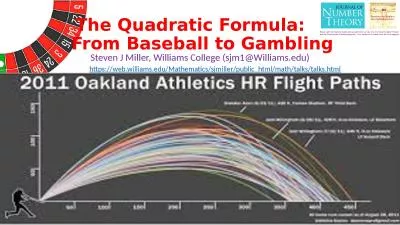
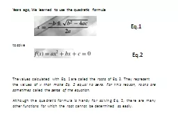
Years ago, We learned to use the quadratic formula - PowerPoint Presentation

Slide1

Years ago, We learned to use the quadratic formula

to solve

The values calculated with Eq. 1 are called the roots of Eq. 2. They represent

the values of

x that make Eq. 2 equal to zero. For this reason, roots are sometimes called the zeros of the equation.Although the quadratic formula is handy for solving Eq. 2, there are many other functions for which the root cannot be determined so easily.

Eq.1

Eq.2Slide2

Before the advent of digital computers, there were a number of ways to solve for the roots of such equations.

For some cases, the roots could be obtained by direct methods, as with Eq. 1.

Although there were equations like this that could be solved directly, there were many more that could not. In such instances, the only alternative is an approximate solution technique.

One method to obtain an approximate solution is to plot the function and determine where it crosses the x axis. This

point, which represents the x value for which f (x) = 0, is the root. Although graphical methods are useful for obtaining rough estimates of roots, they are limited because of their lack of precision. An alternative approach is to use trial and error. This technique consists of guessing a value of x and evaluating whether f (x) is zero. If not (as is almost always the case), another guess is made, and f (x) is again evaluated to determine whether the new value provides a better estimate of the root. The process is repeated until a guess results in an f (x) that is close to zero.Slide3

Numerical methods represent alternatives that are also approximate but employ systematic strategies to home in on the true root. The combination of these systematic methods and computers makes the solution of most applied roots-of-equations problems a simple and efficient task.

There are two methods for locating roots of a single nonlinear equation:

Bracketing

methods for finding roots: These are based on two initial guesses that bracket, or contain,

the root and then systematically reduce the width of the bracket. Two specific methods are covered: bisection and false position. The bracketing methods always work but converge slowly (i.e., they typically take more iterations to home in on the answer).Open methods for finding roots: These methods also involve systematic trial-and-error iterations but do not require that the initial guesses bracket the root. These methods are usually more computationally efficient than bracketing methods but that they do not always work. We will cover several open methods including the

fixed-point iteration, Newton-

Raphson

, and

secant

methods.

Always work (i.e., they can diverge), but when they do they usually converge quicker.Slide4

GRAPHICAL METHODS

A simple method for obtaining an estimate of the root of the equation

f(x) = 0 is to make a plot of the function and observe where it crosses the x axis. This point, which represents the x value for which f(x) = 0, provides a rough approximation of the root.

Graphical techniques are of limited practical value because they are not very precise. However, graphical methods can be utilized to obtain rough estimates of roots. These estimates can be employed as starting guesses for numerical methods.

Graphical interpretations are useful for understanding the properties of the functions and anticipating the pitfalls of the numerical methods.Slide5

Figure shows a number of ways in which roots can occur (or be absent) in an interval prescribed by a lower bound

xl

and an upper bound xu.

Figure (b) depicts the case where a single root is bracketed by negative and positive values of f(x).

Figure (d), where f(xl) and f (xu) are also on opposite sides of the x axis, shows three roots occurring within the interval. In general, if f(xl) and f (xu) have opposite signs, there are an odd number of roots in the interval.

As indicated by Fig. (a) and (c), if

f (xl)

and

f (

xu

)

have the same sign, there are either no roots or an even number of roots between the values.Slide6

For example, functions that are tangential to the

x

axis Fig. (a) and discontinuous functions Fig. (b) can violate these principles. An example of a function that is tangential to the axis is the cubic equation

f (x) = (x − 2)(x − 2

)(x − 4). Notice that x = 2 makes two terms in this polynomial equal to zero. Mathematically, x = 2 is called a multiple root, that occur when the function is tangential to the x axis. For this case, although the end points are of opposite signs, there are an even number of axis interceptions for the interval. Discontinuous functions where end points of opposite

sign bracket an even number of roots. Special strategiesare required for determining the roots for these cases.The existence of these makes it difficult to develop foolproof computer algorithms guaranteed to locate all the roots in an interval. However, when used in conjunction with graphical approaches, the numerical methods are extremely useful for solving many problems confronted routinely by engineers, scientists, and applied mathematicians.Slide7

BISECTION

The bisection method is a variation of the incremental search method in which the interval is always divided in half. If a function changes sign over an interval, the function value at the midpoint is evaluated. The location of the root is then determined as lying within the subinterval where the sign change occurs. The subinterval then becomes the interval for the next iteration. The process is repeated until the root is known to the required precisionSlide8
Slide9
Slide10

METHOD OF FALSE POSITION (

REGULA FALSI)False position (also called the linear interpolation method) is another well-known bracketing method. It is very similar to bisection with the exception that it uses a different strategy to come up with its new root estimate. Rather than bisecting the interval, it locates the root by joining

f(xl) and f(xu

) with a straight line. The intersection of this line with the x axis represents an improved estimate of the root. Thus, the shape of the function influences the new root estimate. Using similar triangles, the intersection of the straight line with the

x axis can be estimated.

This is the false-position formula. The value of xr computed with Eq. then replaces whichever of the two initial guesses,

xl

or

xu

, yields a function value with the same sign as

f (

xr

)

. In this way the values of

xl

and

xu

always bracket the true root. The process is repeated until the root is estimated adequately. The algorithm is identical to the one for bisection with the exception that the above Eq. is used.Slide11
Slide12
Slide13
Slide14

Applied Numerical Methods with MATLAB for Engineers and Scientists

Steven Chapra