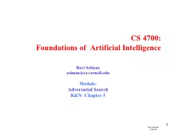
Prof Bart Selman selmancscornelledu Machine Learning Decision Trees RampN 183 Big Data Sensors Everywhere Data collected and stored at enormous speeds GBhour Cars Cellphones ID: 759708
Download Presentation The PPT/PDF document "CS 4700: Foundations of Artificial Inte..." is the property of its rightful owner. Permission is granted to download and print the materials on this web site for personal, non-commercial use only, and to display it on your personal computer provided you do not modify the materials and that you retain all copyright notices contained in the materials. By downloading content from our website, you accept the terms of this agreement.
Slide1
CS 4700:Foundations of Artificial Intelligence
Prof. Bart Selman
selman@cs.cornell.edu
Machine Learning:
Decision
Trees
R&N 18.3
Slide2Big Data:Sensors Everywhere
Data collected and stored at enormous speeds (GB/hour)CarsCellphonesRemote ControlsTraffic lights,ATM machinesAppliancesMotion sensorsSurveillance camerasetc etc
Slide3Big Data:
Scientific Domains
Data collected and stored at
enormous speeds (GB/hour)
remote sensors on a satellite
telescopes scanning the skies
microarrays generating gene
expression data
scientific simulations
generating terabytes of data
Traditional statistical techniques infeasible to deal with the data TUSNAMI – they don’t scale up!!!
Machine Learning Techniques
(adapted from
Vipin
Kumar)
Slide4Machine Learning Tasks
Prediction Methods
Use some variables to predict unknown or future values of other variables.
Description Methods
Find human-interpretable patterns that describe the data.
Slide5Machine Learning Tasks
Supervised learning:
We are given a set of examples with the correct answer - classification
and regression
Unsupervised
learning:
“
just make sense of the data
”
Slide66
Example: Supervised Learningobject recognitionClassification
x
f(x
)
Target
Function
giraffe
giraffe
giraffe
llama
llama
llama
From: Stuart
Russell
Slide77
Example: Supervised Learningobject recognitionClassification
x
giraffe
giraffe
giraffe
llama
llama
llama
X=
f(x)=?
From: Stuart
Russell
f(x
)
Target
Function
Slide8Classifying Galaxies
Early
Intermediate
Late
Data Size:
72 million stars, 20 million galaxies
Object Catalog: 9 GB
Image Database: 150 GB
Class: Stages of Formation
Attributes:Image features, Characteristics of light waves received, etc.
Courtesy: http://aps.umn.edu
Slide9Supervised learning: curve fittingRegression
9
Slide10Supervised learning: curve fittingRegression
10
Slide11Supervised learning: curve fittingRegression
11
Slide12Supervised learning: curve fittingRegression
12
Slide13Supervised learning: curve fittingRegression
13
Slide14Unsupervised Learning:Clustering
14
Ecoregion
Analysis of Alaska using clustering“Representativeness-based Sampling Network Design for the State of Alaska.” Hoffman, Forrest M., Jitendra Kumar, Richard T. Mills, and William W. Hargrove. 2013. Landscape Ecology
Slide15Machine Learning
In
classification
– inputs belong two or more classes.
Goal: the learner
must produce
a model that assigns unseen inputs
to one (or
multi-label classification
) or
more of these classes
. T
ypically supervised learning.
Example –
Spam
filtering is an example of classification, where the inputs are email (or other) messages and the classes are "spam" and "not spam
".
In
regression
, also typically supervised, the
outputs are continuous rather than discrete.
In
clustering
, a set of inputs is to be divided into groups.
Typically done in an
unsupervised
way (i.e., no labels, the
groups are not known
beforehand).
Slide16Supervised learning: Big Picture
Goal: To
learn an unknown
target function
f
Input:
a
training set
of
labeled examples
(
x
j
,y
j
)
where
y
j
= f(
x
j
)
E.g.,
x
j
is an image,
f(
x
j
)
is the label
“
giraffe
”
E.g.,
x
j
is a seismic signal,
f(
x
j
)
is the label
“
explosion
”
Output:
hypothesis
h
that is
“
close
”
to
f
, i.e., predicts well on unseen examples (
“
test set
”
)
Many possible
hypothesis families
for
h
Linear models, logistic regression, neural networks,
support vector machines, decision
trees, examples (nearest-neighbor), grammars,
kernelized
separators,
etc
etc
Slide17Big Picture of Supervised Learning
Learning can be seen as fitting a function to the data. We can consider different target functions and therefore different hypothesis spaces. Examples:Propositional if-then rulesDecision TreesFirst-order if-then rules First-order logic theoryLinear functionsPolynomials of degree at most kNeural networks Java programsTuring machineEtc
Tradeoff between expressiveness of a hypothesis space and the complexity of finding simple, consistent hypotheses within the space.
A learning problemis realizable if its hypothesis space contains the true function.
Today: Decision Trees!
Slide18New York Times
April 16, 2008
Can we learn how counties vote?
Decision Trees:
a sequence of
tests.
Representation very natural for
humans.
Style of many
“
How to
”
manuals
and trouble
-shooting
procedures
.
Slide19Note: order of tests
matters (in general)!
Slide20Decision tree
learning approach
can construct tree
(with test thresholds)
from example counties.
Slide21Decision Tree Learning
Slide22Decision Tree Learning
Input: an object or situation described by a set of attributes (or features) Output: a “decision” – the predicts output value for the input.The input attributes and the outputs can be discrete or continuous.We will focus on decision trees for Boolean classification: each example is classified as positive or negative.
Task:
Given
: collection of examples (x, f(x))
Return
: a function
h
(
hypothesis
) that approximates
f
h
is a
decision tree
Slide23Decision Tree
What is a decision tree?A tree with two types of nodes: Decision nodes Leaf nodes Decision node: Specifies a choice or test of some attribute with 2 or more alternatives; every decision node is part of a path to a leaf nodeLeaf node: Indicates classification of an example
Slide24Big Tip Example
Instance Space X:
Set of all possible objects described by attributes (often called features).
Target Function f: Mapping from Attributes to Target Feature (often called label) (f is unknown)Hypothesis Space H: Set of all classification rules hi we allow.Training Data D: Set of instances labeled with Target Feature
Etc.
Slide25Decision Tree Example: “BigTip”
Food
Price
Speedy
no
yes
no
no
yes
great
mediocre
yuck
yes
no
adequate
high
Is the decision tree we learned consistent?
Yes, it agrees with all the examples
!
Our data
Data: Not all 2x2x3 = 12 tuples
Also, some repeats! These are
literally “observations.”
Slide26Learning decision trees:Another example (waiting at a restaurant)
Problem: decide whether to wait for a table at a restaurant. What attributes would you use?Attributes used by R&NAlternate: is there an alternative restaurant nearby?Bar: is there a comfortable bar area to wait in?Fri/Sat: is today Friday or Saturday?Hungry: are we hungry?Patrons: number of people in the restaurant (None, Some, Full)Price: price range ($, $$, $$$)Raining: is it raining outside?Reservation: have we made a reservation?Type: kind of restaurant (French, Italian, Thai, Burger) WaitEstimate: estimated waiting time (0-10, 10-30, 30-60, >60)
Goal predicate: WillWait?
What about restaurant name?
It could be great for generating a small treebut …
I
t doesn
’
t
generalize!
Slide27Attribute-based representations
Examples described by attribute values (Boolean, discrete, continuous)E.g., situations where I will/won't wait for a table:
Slide28Decision trees
One possible representation for hypotheses
E.g., here is a tree for deciding whether to wait:
Slide29Decision trees can express any Boolean function. Goal: Finding a decision tree that agrees with training set. We could construct a decision tree that has one path to a leaf for each example, where the path tests sets each attribute value to the value of the example. Overall Goal: get a good classification with a small number of tests.
Decision tree learning Algorithm
Problem: This approach would just memorize example. How to deal with new examples? It doesn’t generalize!
We want a compact/smallest tree.But finding the smallest tree consistent with the examples is NP-hard!
(But sometimes hard to avoid --- e.g. parity function, 1, if an even number of inputs, or majority function, 1, if more than half of the inputs are 1).
What is the problem with this from a learning point of view?
Slide30Basic DT Learning Algorithm
Goal: find a small tree consistent with the training examplesIdea: (recursively) choose "most significant" attribute as root of (sub)tree; Use a top-down greedy search through the space of possible decision trees. Greedy because there is no backtracking. It picks highest values first.Variations of known algorithms ID3, C4.5 (Quinlan -86, -93)Top-down greedy constructionWhich attribute should be tested?Heuristics and Statistical testing with current dataRepeat for descendants
(ID3 Iterative Dichotomiser 3)
“most significant”
In what sense?
Slide31Big Tip Example
Let
’s build our decision tree starting with the attribute Food,(3 possible values: g, m, y).
10
8
7
4
3
1
2
5
6
9
10 examples:
6+
4-
Attributes:
Food with values g,m,y
Speedy? with values y,n
Price, with values a, h
Slide32Top-Down Induction of Decision Tree:
Big Tip Example
10 examples:
Food
y
g
m
How many + and - examples
per subclass, starting with y?
6+
4-
10
8
7
4
3
1
2
5
6
9
6
10
8
7
4
3
1
2
5
9
No
No
Let
’
s consider next
the attribute Speedy
Speedy
y
n
10
8
7
3
1
4
2
Yes
Price
a
h
4
2
Yes
No
Node “done” when uniform label, “no
further
Uncertainty,” or no features left
Slide33Top-Down Induction
of DT (simplified)
TDIDF(D,cdef)IF(all examples in D have same class c)Return leaf with class c (or class cdef, if D is empty)ELSE IF(no attributes left to test)Return leaf with class c of majority in DELSEPick A as the “best” decision attribute for next nodeFOR each value vi of A create a new descendent of node Subtree ti for vi is TDIDT(Di,cdef)RETURN tree with A as root and ti as subtrees
Training Data:
Yes
Slide34Picking the Best Attribute to Split
Ockham’s Razor:All other things being equal, choose the simplest explanationDecision Tree Induction:Find the smallest tree that classifies the training data correctlyProblemFinding the smallest tree is computationally hard !ApproachUse heuristic search (greedy search)
Key Heuristics:Pick attribute that maximizes information (Information Gain) i.e. “most informative”Other statistical tests
Slide35Attribute-based representations
Examples described by attribute values (Boolean, discrete, continuous)E.g., situations where I will/won't wait for a table:
Slide36Choosing an attribute:Information Gain
Which one should we pick?
A perfect attribute would
ideally
divide the examples into sub-sets that are all positive or all negative…i.e. maximum information gain.
Is this a good attributeto split on?
Goal: trees with short paths to leaf nodes
Slide37Information Gain
Most useful in classificationhow to measure the ‘worth’ of an attribute information gainhow well attribute separates examples according to their classificationNextprecise definition for gain
Shannon and Weaver 49
measure from Information Theory
One of the most successful and impactful
mathematical theories known.
Slide38Information
“Information” answers questions. Entropy is a measure of unpredictability of information content.The more clueless I am about a question, the more information the answer to the question contains. Example – fair coin prior <0.5,0.5> By definition Information of the prior (or entropy of the prior): I(P1,P2) = - P1 log2(P1) –P2 log2(P2) = I(0.5,0.5) = -0.5 log2(0.5) – 0.5 log2(0.5) = 1We need 1 bit to convey the outcome of the flip of a fair coin.Why does a biased coin have less information?
Scale: 1 bit = answer to Boolean question with prior <0.5, 0.5>
log
2
E
[-log
2
(P(x))]
Slide39Information(or Entropy)
Information in an answer given possible answers v1, v2, … vn:
Example – biased coin prior <1/100,99/100> I(1/100,99/100) = -1/100 log2(1/100) –99/100 log2(99/100) = 0.08 bits (so not much information gained from “answer.”)Example – fully biased coin prior <1,0> I(1,0) = -1 log2(1) – 0 log2(0) = 0 bits
0 log2(0) =0
i.e., no uncertainty left in source!
(Also called
entropy
of the prior.)
Slide40Shape of Entropy Function
Roll of an unbiased die
The more uniform the probability distribution, the greater is its entropy.
0
1
0
1/2
1
p
Slide41Information or Entropy
Information or Entropy measures the “randomness” of an arbitrary collection of examples.We don’t have exact probabilities but our training data provides an estimate of the probabilities of positive vs. negative examples given a set of values for the attributes.For a collection S, entropy is given as: For a collection S having positive and negative examples p - # positive examples; n - # negative examples
Slide42Attribute-based representations
Examples described by attribute values (Boolean, discrete, continuous)E.g., situations where I will/won't wait for a table:
Slide43Choosing an attribute:Information Gain
Intuition: Pick the attribute that reduces the entropy (the uncertainty) the most.So we measure the information gain after testing a given attribute A:
Remainder(A)
gives us
the remaining uncertainty
after getting info on attribute A.
Slide44Choosing an attribute:Information Gain
Remainder(A) gives us the amount information we still need after testing on A.Assume A divides the training set E into E1, E2, … Ev, corresponding to the different v distinct values of A.Each subset Ei has pi positive examples and ni negative examples.So for total information content, we need to weigh the contributions of the different subclasses induced by A
Weight
(relative size) of
each subclass
Slide45Choosing an attribute:Information Gain
Measures the expected reduction in entropy. The higher the Information Gain (IG), or just Gain, with respect to an attribute A , the more is the expected reduction in entropy. where Values(A) is the set of all possible values for attribute A, Sv is the subset of S for which attribute A has value v.
Weight of each subclass
Slide46Interpretations of gain
Gain(S,A)expected reduction in entropy caused by knowing Ainformation provided about the target function value given the value of Anumber of bits saved in the coding a member of S knowing the value of A
Used in ID3 (
Iterative
Dichotomiser
3
) Ross Quinlan
Slide47Information gain
For the training set, p = n = 6, I(6/12, 6/12) = 1 bitConsider the attributes Type and Patrons:Patrons has the highest IG of all attributes and so is chosen by the DTL algorithm as the root.
Info gain?
0.541 bits
Slide48Example contd.
Decision tree learned from the 12 examples:
Substantially simpler than
“
true” tree ---but a more complex hypothesis isn’t justifiedfrom just the data.
“
personal
R&N
Tree
”
Slide49Expressiveness of Decision Trees
Any particular decision tree hypothesis for WillWait goal predicate can be seen as a disjunction of a conjunction of tests, i.e., an assertion of the form: s WillWait(s) (P1(s) P2(s) … Pn(s))Where each condition Pi(s) is a conjunction of tests corresponding to the path from the root of the tree to a leaf with a positive outcome.
Slide50Expressiveness
Decision trees can express any Boolean function of the input attributes.E.g., for Boolean functions, truth table row → path to leaf:
Slide51Expressiveness:Boolean Function with 2 attributes DTs
A
B
B
F
F
T
F
T
F
T
F
T
F
A
B
B
T
F
T
F
T
F
T
F
T
F
A
B
B
T
F
T
T
T
F
T
F
T
F
A
B
B
T
T
F
T
T
F
T
F
T
F
A
B
B
F
F
T
T
T
F
T
F
T
F
A
B
B
F
T
F
T
T
F
T
F
T
F
A
B
B
F
T
F
F
T
F
T
F
T
F
A
B
B
T
T
F
F
T
F
T
F
T
F
AND
OR
XOR
A
NAND
NOR
XNOR
NOT A
2
2
2
Slide52Expressiveness:2 attribute DTs
A
B
F
T
F
T
F
T
F
A
B
B
T
F
T
F
T
F
T
F
T
F
A
B
T
F
T
T
F
F
T
A
B
T
F
T
T
F
T
F
A
F
T
T
F
A
B
B
F
T
F
T
T
F
T
F
T
F
A
B
F
T
F
T
F
F
T
A
T
F
T
F
AND
OR
XOR
NAND
NOR
A
XNOR
NOT A
2
2
2
Slide53A
B
B
F
F
F
T
T
F
T
F
T
F
A
B
B
T
F
T
F
T
F
T
F
T
F
A
B
B
T
F
F
F
T
F
T
F
T
F
A
B
B
T
T
T
F
T
F
T
F
T
F
A
B
B
F
T
F
T
T
F
T
F
T
F
A
B
B
T
T
T
T
T
F
T
F
T
F
A
B
B
F
T
T
T
T
F
T
F
T
F
A
B
B
F
F
F
F
T
F
T
F
T
F
A AND-NOT B
NOT A AND B
B
A OR NOT B
NOR A OR B
TRUE
FALSE
NOT B
Expressiveness:
2 attribute
DTs
2
2
2
Slide54A
B
F
F
T
T
F
T
F
A
B
T
F
F
T
F
F
T
A
B
T
T
F
T
F
T
F
T
A
B
F
T
T
T
F
F
T
F
A AND-NOT B
NOT A AND B
B
A OR NOT B
NOR A OR B
TRUE
FALSE
NOT B
Expressiveness:
2 attribute
DTs
2
2
2
B
F
T
T
F
B
T
F
T
F
Slide55Number of Distinct Decision Trees
How many distinct decision trees with 10 Boolean attributes?= number of Boolean functions with 10 propositional symbolsInput features Output0 0 0 0 0 0 0 0 0 0 0/10 0 0 0 0 0 0 0 0 1 0/10 0 0 0 0 0 0 0 1 0 0/10 0 0 0 0 0 0 1 0 0 0/1…1 1 1 1 1 1 1 1 1 1 0/1
How many entries does this table have?
2
10
So how many Boolean functions
with 10 Boolean attributes are there,given that each entry can be 0/1?
= 2
2
10
Slide56Hypothesis spaces
How many distinct decision trees with n Boolean attributes?= number of Boolean functions= number of distinct truth tables with 2n rows With 6 Boolean attributes, there are 18,446,744,073,709,551,616 possible trees!
= 22n
Googles calculator could not handle 10 attributes !
E.g. how many Boolean functions on 6 attributes? A lot…
Slide57Evaluation
Methodology
General for
Machine Learning
Slide58Evaluation Methodology
Standard methodology (“Holdout Cross-Validation”):1. Collect a large set of examples.2. Randomly divide collection into two disjoint sets: training set and test set.3. Apply learning algorithm to training set generating hypothesis h4. Measure performance of h w.r.t. test set (a form of cross-validation) measures generalization to unseen data Important: keep the training and test sets disjoint! “No peeking”!Note: The first two questions about any learning result: Can you describeyour training and your test set? What’s your error on the test set?
How to evaluate the quality of a learning algorithm, i.e.,:
How good are the hypotheses produce by the learning algorithm?
How good are they at classifying unseen examples?
Slide59Test/Training Split
Real-world Process
(x1,y1), …, (xn,yn)
Learner
(x1,y1),…(xk,yk)
Training Data
D
train
Test Data
D
test
split randomly
split randomly
h
Dtrain
Data D
drawn randomly
Also validation set for meta-
parametres
.
Slide60Measuring Prediction Performance
Slide61Performance Measures
Error Rate
Fraction (or percentage) of false predictions
Accuracy
Fraction (or percentage) of correct predictions
Precision/Recall
Example: binary
classification
problems (classes
pos
/
neg
)
Precision:
Fraction (or percentage) of
correct predictions
among all examples
predicted to be positive
Recall
: Fraction (or percentage) of
correct predictions
among all
real positive
examples
(Can be generalized to multi-class case.)
Slide62Extensions of the Decision Tree Learning Algorithm
Noisy data
Overfitting
and Model Selection
Cross Validation
Missing Data
(R&N, Section 18.3.6)
Using
gain ratios
(R&N, Section 18.3.6)
Real
-valued
data (R&N, Section 18.3.6)
Generation of
rules and pruning
DT Ensembles
Regression DT
Slide63How well does it work?
Many case studies have shown that decision trees are at least as accurate as human experts.
A study for
diagnosing breast cancer
had
humans
correctly classifying the examples
65%
of the time, and the
decision tree
classified
72%
correct.
British Petroleum
designed a
decision tree for gas-oil separation for offshore oil platforms
that replaced an earlier rule-based expert system.
Cessna
designed an
airplane flight controller
using
90,000 examples and 20 attributes
per example.
Bird Distributions Machine Learning and Citizen Science
Adaptive Spatio-Temporal Machine Learning Models and Algorithms(STEM Models)Relate environmental predictors to observed patterns of occurrences and absences
Land Cover
Weather
Remote
Sensing
Environmental Data
Patterns of occurrence
of
the Tree Swallow for different months of the year
Source : Daniel Fink
80,000
+
CPU Hours
(~ 10 Years!!!)
Bird Observations
State of the Birds
Report
(officially released by Secretary of Interior)
Bird Distribution Models, Revealing, at a fine resolution, Species’ Habitat Preferences
Novel Approaches
To Conservation
Based on
eBird
Models
300K+
volunteer birders
300M+
bird observations
22M+
hours of field work
(
2500+years)
Distribution Models for
400+ species with
weekly estimates at fine spatial resolution(3km2)
Boosted Regression
DT Ensemble
Slide65Summary:When to use Decision Trees
Instances presented as attribute-value pairsMethod of approximating discrete-valued functions Target function has discrete values: classification problemsRobust to noisy data: Training data may contain errorsmissing attribute valuesTypical bias: prefer smaller trees (Ockham's razor )
Widely used, practical and easy to interpret results
Slide66Inducing decision trees is one of the most widely used learning methods in practice Can outperform human experts in many problems Strengths includeFastsimple to implementhuman readablecan convert result to a set of easily interpretable rulesempirically valid in many commercial productshandles noisy data Weaknesses include:"Univariate" splits/partitioning using only one attribute at a time so limits types of possible treeslarge decision trees may be hard to understandrequires fixed-length feature vectors non-incremental (i.e., batch method)
Can be a legal requirement! Why?