PPT-Lecture 6A – Introduction to Trees & Optimality Criteria

Author : goldengirl | Published Date : 2020-06-17

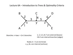
Branches n taxa gt 2 n 3 branches 1 2 4 6 amp 7 are external leaves 3 amp 5 are internal branches edges Nodes A E are terminals x y amp z are internal vertices

Presentation Embed Code

Download Presentation

Download Presentation The PPT/PDF document "Lecture 6A – Introduction to Trees &am..." is the property of its rightful owner. Permission is granted to download and print the materials on this website for personal, non-commercial use only, and to display it on your personal computer provided you do not modify the materials and that you retain all copyright notices contained in the materials. By downloading content from our website, you accept the terms of this agreement.

Lecture 6A – Introduction to Trees & Optimality Criteria: Transcript

Branches n taxa gt 2 n 3 branches 1 2 4 6 amp 7 are external leaves 3 amp 5 are internal branches edges Nodes A E are terminals x y amp z are internal vertices . http://www.fallenleaftree.com For a lot of people, their home is there most important investment they can make. Having a well maintained landscape is important to the overall property because it’s the first impression everybody gets. (Part 1). Daniel Kirschen. Economic . d. ispatch problem. Several generating units serving the load. What share of the load should each generating unit produce?. Consider the limits of the generating units. Baldrige Performance Excellence Program | www.nist.gov/baldrige. It . amazes me that U.S. businesses spend so much money on . “how-to” . books and . course work . to teach leaders how to build successful organizations. . Dwyane George. February 24, 2015. 18.434. Outline. Introduction & Motivation. Definition. Algorithm & Proof of Correctness. Unweighted. Pair Group Method with Arithmetic Mean (UPGMA). Algorithm Runtime. Approximate Algorithms. Alessandro Farinelli. Approximate Algorithms: outline. No guarantees. DSA-1, MGM-1 (exchange individual assignments). Max-Sum (exchange functions). Off-Line guarantees. K-optimality and extensions. CS/CNS/EE 155. Lecture 3:. Regularization, Sparsity & Lasso. 1. Homework 1. Check course website!. Some coding required. Some plotting . required. I recommend . Matlab. Has supplementary datasets. Tandy Warnow. Joint work with . Siavash. . Mirarab. , . Md. S. . Bayzid. , and others. Orangutan. Gorilla. Chimpanzee. Human. From the Tree of the Life Website. ,. . University . of . Arizona. Dates from Lock et al. Nature, 2011. NYC Watershed/. Tifft. Scientific and Technical Symposium. Ron . Entringer. w/Cliff . Callinan. Scott . Kishbaugh. NYSDEC Division of Water. September 19, 2013. Bridge Between. SWDA & CWA. Waste Load . Presented by ALIA Students and New Graduates Group (SNGG). Event Program. Introduction. Kylie Tran – The University of Melbourne. Georgina Earl – Whitehorse Manningham Libraries. Deborah Tout-Smith – Museum Victoria. Dr. Halimah Alshehri. 1. Introduction to Trees. DEFINITION 1 . A . tree. is a connected undirected graph with no simple circuits.. Because . a tree cannot have a simple circuit. , . a tree cannot contain multiple edges or loops. MISSION. GET INVOLVED. DONATE. ‘. Discover, educate, serve & inspire. ’ . NEWS & EVENTS. GARDEN PARTNERS. Research. : The UA Campus Arboretum is built upon the historical priorities of the Land Grant . Sultan Almuhammadi ICS 254: Graphs and Trees 1 Graph & Trees Chapters 10-11 Acknowledgement This is a modified version of Module#22 on Graph Theory by Michael Frank Sultan Almuhammadi ICS 254: Graphs and Trees C. linical . D. ecision . M. aking . Faith Rialem . Class of 2018. Objectives. Calculations. Maintenance fluids. Winters formula. Anion Gap. Corrected QT. Absolute neutrophil count. Criteria. Centor criteria. Identification . of . Dynamic Models . of . Biosystems. Julio R. . Banga. IIM-CSIC, Vigo, . Spain. julio@iim.csic.es. CUNY-Courant Seminar in Symbolic-Numeric Computing. CUNY . Graduate. . Center. , Friday, .

Download Document

Here is the link to download the presentation.
"Lecture 6A – Introduction to Trees & Optimality Criteria"The content belongs to its owner. You may download and print it for personal use, without modification, and keep all copyright notices. By downloading, you agree to these terms.