PDF-The Empirical Relationship betweenAverage Asset Correlation Firm Prob

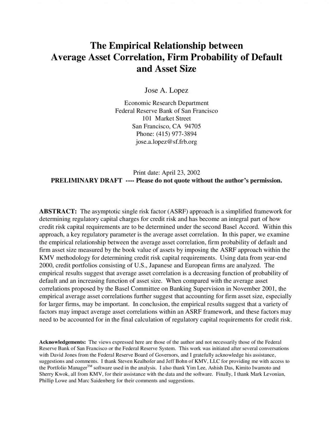
See Gordy 2000a b for further discussion of the ASRF approach The software firm KMV LLC is a leader in the field of credit risk modeling and capital budgeting Thisstudy

values asset portfolios edf asset values edf portfolios average size firms calibrated portfolio categories 20000 based correlation correlations 10000

Presentation Embed Code

<iframe width="560" height="315" src="https://www.docslides.com/embed/953019" frameborder="0" allowfullscreen></iframe>

Download Presentation

Download Presentation The PPT/PDF document "The Empirical Relationship betweenAverag..." is the property of its rightful owner. Permission is granted to download and print the materials on this web site for personal, non-commercial use only, and to display it on your personal computer provided you do not modify the materials and that you retain all copyright notices contained in the materials. By downloading content from our website, you accept the terms of this agreement.