/
Bayes net global semantics Bayes net global semantics

Bayes net global semantics - PowerPoint Presentation

jocelyn
jocelyn . @jocelyn
Follow
66 views
Uploaded On 2023-05-19

Bayes net global semantics - PPT Presentation

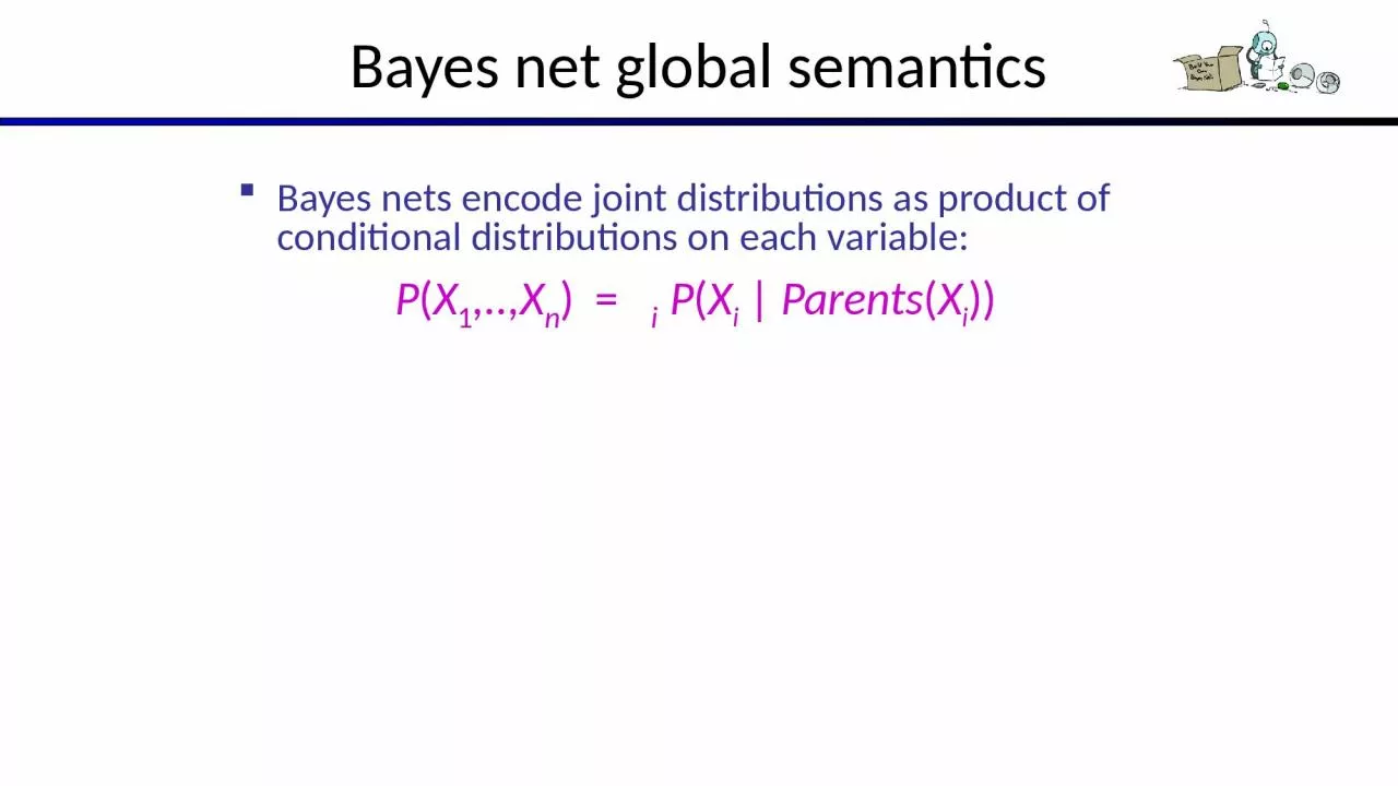
Bayes nets encode joint distributions as product of conditional distributions on each variable P X 1 X n i P X i Parents X i PB true false 0001 ID: 997877

variable factor joint conditional factor variable conditional joint jtruefalsetrue0 bayes elimination parents product factors 1false0 090 variables complexity numbers

Share:

Link:

Embed:

Download Presentation from below link

Download Presentation The PPT/PDF document "Bayes net global semantics" is the property of its rightful owner. Permission is granted to download and print the materials on this web site for personal, non-commercial use only, and to display it on your personal computer provided you do not modify the materials and that you retain all copyright notices contained in the materials. By downloading content from our website, you accept the terms of this agreement.


Presentation Transcript

1. Bayes net global semanticsBayes nets encode joint distributions as product of conditional distributions on each variable:P(X1,..,Xn) = i P(Xi | Parents(Xi))

2. P(B)truefalse0.0010.999ExampleP(b,e, a, j, m) =2BEP(A|B,E)truefalsetruetrue0.950.05truefalse0.940.06falsetrue0.290.71falsefalse0.0010.999AP(J|A)truefalsetrue0.90.1false0.050.95P(E)truefalse0.0020.998AP(M|A)truefalsetrue0.70.3false0.010.99P(b) P(e) P(a|b,e) P(j|a) P(m|a) =.001x.998x.94x.1x.3=.000028 BurglaryEarthquakeAlarmJohn callsMary calls

3. Conditional independence in BNsCompare the Bayes net global semantics P(X1,..,Xn) = i P(Xi | Parents(Xi)) with the chain rule identity P(X1,..,Xn) = i P(Xi | X1,…,Xi-1)Assume (without loss of generality) that X1,..,Xn sorted in topological order according to the graph (i.e., parents before children), so Parents(Xi)  X1,…,Xi-1So the Bayes net asserts conditional independences P(Xi | X1,…,Xi-1) = P(Xi | Parents(Xi))To ensure these are valid, choose parents for node Xi that “shield” it from other predecessors

4. Conditional independence semanticsEvery variable is conditionally independent of its non-descendants given its parentsConditional independence semantics <=> global semantics4

5. Example: BurglaryBurglaryEarthquakeAlarm5BurglaryEarthquakeAlarm???P(B)truefalse0.0010.999BEP(A|B,E)truefalsetruetrue0.950.05truefalse0.940.06falsetrue0.290.71falsefalse0.0010.999P(E)truefalse0.0020.998

6. Example: BurglaryAlarmBurglaryEarthquake6BurglaryEarthquakeAlarm???P(A)truefalseABP(E|A,B)truefalsetruetruetruefalsefalsetruefalsefalseAP(B|A)truefalsetruefalse??

7. SummaryIndependence and conditional independence are important forms of probabilistic knowledgeBayes net encode joint distributions efficiently by taking advantage of conditional independenceGlobal joint probability = product of local conditionalsExact inference = sums of products of conditional probabilities from the network

8. CS 188: Artificial IntelligenceBayes Nets: Exact InferenceInstructor: Stuart Russell and Dawn Song --- University of California, Berkeley

9. Examples:Posterior marginal probabilityP(Q|e1,..,ek) E.g., what disease might I have?Most likely explanation:argmaxq,r,s P(Q=q,R=r,S=s|e1,..,ek)E.g., what did they say? InferenceInference: calculating some useful quantity from a probability model (joint probability distribution)

10. Inference by Enumeration in Bayes NetReminder of inference by enumeration:Any probability of interest can be computed by summing entries from the joint distribution: P(Q | e) =  h P(Q , h, e)Entries from the joint distribution can be obtained from a BN by multiplying the corresponding conditional probabilitiesP(B | j, m) = α e,a P(B, e, a, j, m) = α e,a P(B) P(e) P(a|B,e) P(j|a) P(m|a)So inference in Bayes nets means computing sums of products of numbers: sounds easy!!Problem: sums of exponentially many products!BEAMJ

11. Can we do better?Consider uwy + uwz + uxy + uxz + vwy + vwz + vxy +vxz 16 multiplies, 7 addsLots of repeated subexpressions!Rewrite as (u+v)(w+x)(y+z)2 multiplies, 3 addse,a P(B) P(e) P(a|B,e) P(j|a) P(m|a)= P(B)P(e)P(a|B,e)P(j|a)P(m|a) + P(B)P(e)P(a|B,e)P(j|a)P(m|a) + P(B)P(e)P(a|B,e)P(j|a)P(m|a) + P(B)P(e)P(a|B,e)P(j|a)P(m|a) Lots of repeated subexpressions!11

12. Variable elimination: The basic ideasMove summations inwards as far as possibleP(B | j, m) = α e,a P(B) P(e) P(a|B,e) P(j|a) P(m|a) = α P(B) e P(e) a P(a|B,e) P(j|a) P(m|a)Do the calculation from the inside outI.e., sum over a first, then sum over eProblem: P(a|B,e) isn’t a single number, it’s a bunch of different numbers depending on the values of B and eSolution: use arrays of numbers (of various dimensions) with appropriate operations on them; these are called factors12

13. Factor Zoo

14. Factor Zoo IJoint distribution: P(X,Y)Entries P(x,y) for all x, y|X|x|Y| matrixSums to 1Projected joint: P(x,Y)A slice of the joint distributionEntries P(x,y) for one x, all y|Y|-element vectorSums to P(x)A \ Jtruefalsetrue0.090.01false0.0450.855P(A,J)P(a,J) = Pa(J)Number of variables (capitals) = dimensionality of the tableA \ Jtruefalsetrue0.090.01

15. Factor Zoo IISingle conditional: P(Y | x)Entries P(y | x) for fixed x, all ySums to 1Family of conditionals: P(X |Y)Multiple conditionalsEntries P(x | y) for all x, ySums to |Y|A \ Jtruefalsetrue0.90.1P(J|a)A \ Jtruefalsetrue0.90.1false0.050.95P(J|A)} - P(J|a)} - P(J|a)

16. Operation 1: Pointwise productFirst basic operation: pointwise product of factors (similar to a database join, not matrix multiply!)New factor has union of variables of the two original factorsEach entry is the product of the corresponding entries from the original factorsExample: P(J|A) x P(A) = P(A,J)P(J|A)P(A)P(A,J)A \ Jtruefalsetrue0.090.01false0.0450.855A \ Jtruefalsetrue0.90.1false0.050.95true0.1false0.9x=

17. Example: Making larger factorsExample: P(A,J) x P(A,M) = P(A,J,M)P(A,J)A \ Jtruefalsetrue0.090.01false0.0450.855x=P(A,M)A \ Mtruefalsetrue0.070.03false0.0090.891A=trueA=falseP(A,J,M)

18. Example: Making larger factorsExample: P(U,V) x P(V,W) x P(W,X) = P(U,V,W,X)Sizes: [10,10] x [10,10] x [10,10] = [10,10,10,10] I.e., 300 numbers blows up to 10,000 numbers!Factor blowup can make VE very expensive

19. Operation 2: Summing out a variableSecond basic operation: summing out (or eliminating) a variable from a factorShrinks a factor to a smaller oneExample: j P(A,J) = P(A,j) + P(A,j) = P(A) A \ Jtruefalsetrue0.090.01false0.0450.855true0.1false0.9P(A)P(A,J)Sum out J

20. Summing out from a product of factorsProject the factors each way first, then sum the productsExample: a P(a|B,e) x P(j|a) x P(m|a) = P(a|B,e) x P(j|a) x P(m|a) + P(a|B,e) x P(j|a) x P(m|a)

21. Variable Elimination

22. Variable EliminationQuery: P(Q|E1=e1,.., Ek=ek) Start with initial factors:Local CPTs (but instantiated by evidence)While there are still hidden variables (not Q or evidence):Pick a hidden variable HjEliminate (sum out) Hj from the product of all factors mentioning HjJoin all remaining factors and normalizeX α

23. ExampleChoose AP(B) P(E) P(A|B,E) P(j|A) P(m|A)Query P(B | j,m) P(A|B,E) P(j|A)P(m|A)P(j,m|B,E)P(B) P(E) P(j,m|B,E)

24. ExampleNormalizeChoose EP(E) P(j,m|B,E)P(j,m|B)P(B) P(E) P(j,m|B,E)Finish with BP(B) P(j,m|B)P(j,m,B)P(B) P(j,m|B)P(B | j,m)

25. Order mattersOrder the terms Z, A, B C, DP(D) = α z,a,b,c P(z) P(a|z) P(b|z) P(c|z) P(D|z) = α z P(z) a P(a|z) b P(b|z) c P(c|z) P(D|z)Largest factor has 2 variables (D,Z)Order the terms A, B C, D, ZP(D) = α a,b,c,z P(a|z) P(b|z) P(c|z) P(D|z) P(z) = α a b c z P(a|z) P(b|z) P(c|z) P(D|z) P(z)Largest factor has 4 variables (A,B,C,D)In general, with n leaves, factor of size 2nDZABC

26. VE: Computational and Space ComplexityThe computational and space complexity of variable elimination is determined by the largest factor (and it’s space that kills you)The elimination ordering can greatly affect the size of the largest factor. E.g., previous slide’s example 2n vs. 2Does there always exist an ordering that only results in small factors?No!

27. Worst Case Complexity? Reduction from SATVariables: W, X, Y, ZCNF clauses:C1 = W v X v YC2 = Y v Z v  WC3 = X v Y v ZSentence S = C1  C2  C3P(S) > 0 iff S is satisfiable=> NP-hardP(S) = K x 0.5n where K is the number of satisfying assignments for clauses=> #P-hardSC1C2C3  WXYZ0.50.50.50.5

28. PolytreesA polytree is a directed graph with no undirected cyclesFor poly-trees the complexity of variable elimination is linear in the network size if you eliminate from the leave towards the roots

29. Bayes NetsPart I: RepresentationPart II: Exact inferenceEnumeration (always exponential complexity)Variable elimination (worst-case exponential complexity, often better)Inference is NP-hard in generalPart III: Approximate InferenceLater: Learning Bayes nets from data