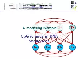
G T A C G T A modeling Example CpG islands in DNA sequences Methylation amp Silencing One way cells differentiate is methylation Addition of CH 3 in Cnucleotides Silences genes in region ID: 139681
Download Presentation The PPT/PDF document "A+ C+" is the property of its rightful owner. Permission is granted to download and print the materials on this web site for personal, non-commercial use only, and to display it on your personal computer provided you do not modify the materials and that you retain all copyright notices contained in the materials. By downloading content from our website, you accept the terms of this agreement.
Slide1
A+
C+
G+
T+
A-
C-
G-
T-
A modeling Example
CpG islands in DNA sequencesSlide2
Methylation & Silencing
One way cells differentiate is methylationAddition of CH3
in C-nucleotidesSilences genes in regionCG (denoted CpG) often mutates to TG, when methylatedIn each cell, one copy of X is silenced, methylation plays role
Methylation is inherited during cell divisionSlide3
Example: CpG Islands
CpG nucleotides in the genome are frequently methylated
(Write CpG not to confuse with CG base pair)
C
methyl-C T
Methylation often suppressed around genes, promoters
CpG islandsSlide4
Example: CpG Islands
In CpG islands,
CG is more frequentOther pairs (AA, AG, AT…) have different frequencies
Question: Detect CpG islands computationallySlide5
A model of CpG Islands – (1) Architecture
A+
C+
G+
T+
A-
C-
G-
T-
CpG Island
Not CpG IslandSlide6
A model of CpG Islands – (2) Transitions
How do we estimate parameters of the model?
Emission probabilities: 1/0Transition probabilities within CpG islands
Established from known CpG islands
(Training Set)Transition probabilities within other regions
Established from known non-CpG islands (Training Set)
Note: these transitions out of each state add up to one—no room for transitions between (+) and (-) states
+
A
C
G
T
A
.180
.274
.426
.120
C
.171
.368
.274
.188
G
.161
.339
.375
.125
T
.079
.355
.384
.182
-
A
C
G
T
A
.300
.205
.285
.210
C
.233
.298
.078
.302
G
.248
.246
.298
.208
T
.177
.239
.292
.292
= 1
= 1
= 1
= 1
= 1
= 1
= 1
= 1Slide7
Log Likehoods—
Telling “CpG Island” from “Non-CpG Island”
A
C
G
T
A
-0.740
+0.419
+0.580
-0.803
C
-0.913
+0.302
+1.812
-0.685
G
-0.624
+0.461
+0.331
-0.730
T
-1.169
+0.573
+0.393
-0.679
Another way to see effects of transitions:
Log likelihoods
L(u, v) = log[ P(uv | + ) / P(uv | -) ]
Given a region x = x
1
…x
N
A quick-&-dirty way to decide whether entire x is CpG
P(x is CpG) > P(x is not CpG)
i
L(x
i
, x
i+1
) > 0Slide8
A model of CpG Islands – (2) Transitions
What about transitions between (+) and (-) states?They affect
Avg. length of CpG islandAvg. separation between two CpG islands
X
Y
1-p
1-q
p
q
Length distribution of region X:
P[l
X
= 1] = 1-p
P[l
X
= 2] = p(1-p)
…
P[l
X
= k] = p
k-1
(1-p)
E[l
X
] = 1/(1-p)
Geometric distribution, with mean 1/(1-p)Slide9
Applications of the model
Given a DNA region x,
The Viterbi algorithm predicts locations of CpG islandsGiven a nucleotide xi
, (say xi = A)
The Viterbi parse tells whether xi is in a CpG island in the most likely general scenario
The Forward/Backward algorithms can calculate
P(xi is in CpG island) = P(
i = A+ | x)
Posterior Decoding can assign locally optimal predictions of CpG islands
^
i = argmaxk
P(i = k | x)
Advantage: ?Each nucleotide is more likely to be called correctly
Disadvantage: ?The overall parse will be “choppy”—CpG islands too short
Advantage/Disadvantage?Slide10
What if a new genome comes?
We just sequenced the porcupine genomeWe know CpG islands play the same role in this genome
However, we have no known CpG islands for porcupinesWe suspect the frequency and characteristics of CpG islands are quite different in porcupines
How do we adjust the parameters in our model? LEARNINGSlide11
Learning
Re-estimate the parameters of the model based on training dataSlide12
Two learning scenarios
Estimation when the “right answer” is known
Examples: GIVEN:
a genomic region x = x1…x1,000,000 where we have good (experimental) annotations of the CpG islands
GIVEN: the casino player allows us to observe him one evening, as he changes dice and produces 10,000 rolls
Estimation when the “right answer” is unknownExamples:
GIVEN: the porcupine genome; we don’t know how frequent are the CpG islands there, neither do we know their composition
GIVEN: 10,000 rolls of the casino player, but we don’t see when he changes dice
QUESTION: Update the parameters of the model to maximize P(x|
)Slide13
1. When the right answer is known
Given x = x1…xN
for which the true = 1…
N is known,Define:
Akl
= # times kl transition occurs in Ek(b) = # times state k in emits b in x
We can show that the maximum likelihood parameters
(maximize P(x|)) are:
Akl Ek(b)
akl = –––––
ek(b) = –––––––
i Aki
c Ek(c)Slide14
1. When the right answer is known
Intuition: When we know the underlying states,
Best estimate is the normalized frequency of transitions & emissions that occur in the training dataDrawback:
Given little data, there may be overfitting: P(x|
) is maximized, but is unreasonable 0 probabilities – BAD
Example: Given 10 casino rolls, we observe
x = 2, 1, 5, 6, 1, 2, 3, 6, 2, 3
= F, F, F, F, F, F, F, F, F, F Then:
aFF = 1; a
FL = 0 eF(1) = e
F(3) = .2; eF
(2) = .3; eF(4) = 0; eF(5) = e
F(6) = .1 Slide15
Pseudocounts
Solution for small training sets: Add pseudocounts
Akl = # times kl transition occurs in + r
kl Ek(b) = # times state k in emits b in x + r
k(b)rkl, r
k(b) are pseudocounts representing our prior beliefLarger pseudocounts Strong priof belief
Small pseudocounts ( < 1): just to avoid 0 probabilities Slide16
Pseudocounts
Example: dishonest casino
We will observe player for one day, 600 rolls Reasonable pseudocounts:
r0F = r0L = r
F0 = rL0 = 1; r
FL = rLF = rFF
= rLL = 1; rF
(1) = rF(2) = … = rF(6) = 20
(strong belief fair is fair) rL(1) = r
L(2) = … = rL(6) = 5 (wait and see for loaded)
Above #s are arbitrary – assigning priors is an artSlide17
2. When the right answer is unknown
We don’t know the true Akl
, Ek(b)Idea:
We estimate our “best guess” on what Akl, E
k(b) areOr, we start with random / uniform values
We update the parameters of the model, based on our guessWe repeatSlide18
2. When the right answer is unknown
Starting with our best guess of a model M, parameters :
Given x = x1…xN for which the true
= 1…N is unknown,
We can get to a provably more likely parameter set
i.e., that increases the probability P(x | )
Principle: EXPECTATION MAXIMIZATION
Estimate Akl, Ek(b) in the training data
Update according to Akl, Ek
(b)Repeat 1 & 2, until convergenceSlide19
Estimating new parameters
To estimate Akl:
(assume “|
CURRENT”, in all formulas below)
At each position i of sequence x, find probability transition kl is used:
P(i = k, i+1
= l | x) = [1/P(x)] P(i = k,
i+1 = l, x1…xN
) = Q/P(x)where Q = P(x1
…xi, i = k,
i+1 = l, xi+1…xN
) = = P(i+1 = l, xi+1
…xN | i = k) P(x
1…xi, i
= k) = = P(i+1 = l, x
i+1xi+2…xN |
i = k) fk(i) =
= P(xi+2…xN |
i+1 = l) P(xi+1 | i+1
= l) P(i+1 = l | i = k) f
k(i) = = bl(i+1) e
l(xi+1) akl
fk(i)
fk(i) akl e
l(xi+1) bl
(i+1)
So: P(i = k, i+1 = l | x, ) = ––––––––––––––––––
P(x | CURRENT
)Slide20
Estimating new parameters
So, Akl is the E[# times transition
kl, given current ] f
k(i) akl el(x
i+1) bl(i+1)
Akl = i P(
i = k, i+1 = l | x, ) =
i ––––––––––––––––– P(x | )
Similarly,
Ek(b) = [1/P(x | )]
{i | xi = b} f
k(i) bk(i)
k
l
x
i+1
a
kl
e
l
(x
i+1
)
b
l
(i+1)
f
k
(i)
x
1
………x
i-1
x
i+2
………x
N
x
iSlide21
The Baum-Welch Algorithm
Initialization: Pick the best-guess for model parameters
(or arbitrary)Iteration:
ForwardBackwardCalculate
Akl, Ek(b), given
CURRENT
Calculate new model parameters NEW : a
kl, ek(b)
Calculate new log-likelihood P(x | NEW)
GUARANTEED TO BE HIGHER BY EXPECTATION-MAXIMIZATION
Until P(x | ) does not change muchSlide22
The Baum-Welch Algorithm
Time Complexity:
# iterations O(K2N)
Guaranteed to increase the log likelihood P(x | )
Not guaranteed to find globally best parameters
Converges to local optimum, depending on initial conditions
Too many parameters / too large model: OvertrainingSlide23
Alternative: Viterbi Training
Initialization: Same
Iteration:Perform Viterbi, to find
*Calculate A
kl, Ek(b) according to *
+ pseudocountsCalculate the new parameters akl, ek(b)
Until convergenceNotes:
Not guaranteed to increase P(x | )Guaranteed to increase P(x |
, *)In general, worse performance than Baum-Welch