PDF-From Visibilities to Images

Author : kittie-lecroy | Published Date : 2015-12-03

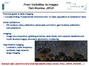
Tom Muxlow JBCA Practical guide to basic imaging x2013 omplimenting x2018Fundamental Interferometryx2019 x2018Data Acquisition alibrationx2019 talks Initial Calibration RFI

Presentation Embed Code

<iframe width="560" height="315" src="https://www.docslides.com/embed/213333" frameborder="0" allowfullscreen></iframe>

Download Presentation

Download Presentation The PPT/PDF document "From Visibilities to Images" is the property of its rightful owner. Permission is granted to download and print the materials on this website for personal, non-commercial use only, and to display it on your personal computer provided you do not modify the materials and that you retain all copyright notices contained in the materials. By downloading content from our website, you accept the terms of this agreement.

From Visibilities to Images: Transcript

Download Document

Here is the link to download the presentation.
"From Visibilities to Images"The content belongs to its owner. You may download and print it for personal use, without modification, and keep all copyright notices. By downloading, you agree to these terms.