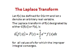
PPT-Using Laplace Transforms to Solve IVPs with Discontinuous Forcing Functions PowerPoint Presentation

MAT 275 Example Find the solution of the IVP Solution Rewrite the forcing function using the notation Now apply the Laplace Transform Operator to both sides and

Upload by kittie-lecroy
Published on 2018-09-21

Presentation Embed Code

<iframe width="560" height="315" src="https://www.docslides.com/embed/674705" frameborder="0" allowfullscreen></iframe>

Download Presentation

Download Presentation The PPT/PDF document "Using Laplace Transforms to Solve IVPs w..." is the property of its rightful owner. Permission is granted to download and print the materials on this web site for personal, non-commercial use only, and to display it on your personal computer provided you do not modify the materials and that you retain all copyright notices contained in the materials. By downloading content from our website, you accept the terms of this agreement.