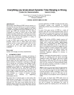
In spite of DTW’s great success, there are still several persiste - PDF document

In spite of DTW’s great success, there are still several persistent “myths” about it. These myths have caused confusion and led to much wasted research effort. In this work, we will dispel these myths with the most comprehensive set of time series experiments ever conducted. The steady flow of research papers on data mining with DTW became a torrent after it was shown that a simple lower bound allowed DTW to be indexed with no false The ability of DTW to handle sequences of different lengths is a great advantage, and therefore the simple lower bound that resequences to be reinterpolated to equal length is of limited utility [18][27][28]. In fact, as we will show, extensive empirical evidence presented here suggests that comparing sequences of different lengths and reinterpolating them to equal length produce no Myth 2 In this paper, we dispel these DTW myths above by empirically demonstrate our findings with a comprehensive set of experiments. In terms of number of objective datasets and size of datasets, our experiments are orders of magnitude greater than anything else in the literature. In particular, our experiments required more than eight billion DTW comparisons. Before beginning our deconstruction of these myths, it would be remiss of us not to note that several early papers by the second author are guilty of echoing them. This work is part of an effort to redress these mistakes. Likewise, we have taken advantage of the informal nature of a workshop to choose a tongue-in-cheek attention grabbing title. We do not really mean to imply that the entire community is ignorant of the intricacies of DTW. The rest of the paper is organized as follows. In Section 2, we give an overview of Dynamic Time Warping (DTW) and its related work. The next three sections consider each of the three myths above. Section 6 suggests some avenues for future researches, and Section 7 gives conclusions and directions for future work. Because we are testing on a wide range of real and synthetic datasets, we have placed the details about them in Appendix A to enhance the flow of the paper. 2. BACKGROUND AND RELATED WORK The measurement of similarity between two time series is an important subroutine in many data mining applications, including classification [11][14], clustering [1][10], anomaly detection [9], rule discovery [8], and motif discovery [7]. The superiority of DTW over Euclidean distance metric for these tasks has been demonstrated by many authors [1][2][5][29]. We will first begin with a review of some background material on DTW and its recent extensions, which contributes to our main motivation of this paper. 2.1 REVIEW OF DTW Suppose we have two time series, a sequence Q of length n, and a sequence C of length m, where Q = q1,q2,…,qi,…,qn (1) C = c1,c2,…,cj,…cm (2) To align these two sequences using DTW, we first construct an n-by-m matrix where the (ith , jth ) element of the matrix corresponds to the squared distance, d(qi , cj) = (qi – cj)2, which is the alignment between points qi and cj. To find the best match between these two sequences, we retrieve a path through the matrix that minimizes the total cumulative distance between them as illustrated in Figure 1. In particular, the optimal path is the path that minimizes the warping cost KkkwCQDTW1min),( (3) where wk is the matrix element (i,j)k that also belongs to kth element of a warping path W, a contiguous set of matrix elements that represent a mapping between Q and C. This warping path can be found using dynamic programming to evaluate the following recurrence. (i,j) = d(qi,cj) + min{ (i-1,j-1) , (i-1,j ) , (i,j-1) } (4) where d(i,j) is the distance found in the current cell, and (i,j) is the cumulative distance of d(i,j) and the minimum cumulative distances from the three adjacent cells. QCA) QCA) B)CQ B)CQ C)CQ C)CQ Figure 1. A) Two similar sequences Q and C, but out of phase. B) To align the sequences, we construct a warping matrix and search for the optimal warping path, shown with solid squares. Note that the 'corners' of the matrix (shown in dark gray) are excluded from the search path as part of an Adjustment Window condition. C) The resulting alignment. To reduce the number of paths to consider during the computation, several well-known constraints (Boundary Conditions, Continuity condition, Monotonic condition, and Adjustment Window Condition) have been applied to the problem to restrict the moves that can be made from any point in the path and so restrict the number of paths that need to be considered. Figure 1 B) illustrates a particular example of the Adjustment Window Condition (or Warping Window Constraints) with the Sakoe-Chiba Band [26]. The width of this constraint is often set to 10% of the length of the time series [1][22][26]. 2.2 LOWER BOUNDING THE DTW DISTANCE A recent extension to DTW that significantly speeds up the DTW calculation is a lower bounding technique based on the warping window (envelope) [15]. CQ Sakoe-Chiba Band CQ Itakura Parallelogram Figure 2. The two most common constraints in the literature are the Sakoe-Chiba Band and the Itakura Parallelogram Figure 2 illustrates two of the most frequently used global constraints in the literature, the Sakoe-Chiba Band [26] and could benefit from wider constraints, we found no evidence for this in a survey of more than 500 papers on the topic. More tellingly, in spite of extensive efforts, we could not even create a large synthetic dataset for classification that needs more than 10% warping. All the evidence suggests that narrow constraints are necessary for accurate DTW, and the “need” to support wide (or no) constraints is just a myth. 5. CAN DTW BE FURTHER SPEEDED UP? Smaller warping windows speed up the DTW calculations simply because there is less area of the warping matrix to be searched. Prior to the introduction of lower bounding, the amount of speedup was directly proportional to the width of the warping window. For example, a nearest neighbor search with a 10% warping constraint was almost exactly twice as fast as a search done with a 20% window. However, it is important to note that with the introduction of lower bounding based on warping constraints (i.e. 4S), the speedup is now highly nonlinear in the size of the warping window. For example, a nearest neighbor search with a 10% warping constraint may be many times faster than twice a search done with a 20% window. In spite of this, many recent papers still claim that there is a need and room for further improvement in speeding up DTW. For example, a recent paper suggested “dynamic time warping incurs a heavy CPU cost…” Surprisingly, as we will now show, the amortized CPU cost of DTW is essentially O(n) if we use the trivial 4S technique. To really understand what is going on, we will avoid measuring the efficiency of DTW when using index structures. The use of such index structures opens the possibility of implementation bias [17]; it is simply difficult to know if the claimed speedup truly reflects a clever algorithm, or simply the care in choice of buffer size, caching policy, etc. Instead, we measure the computation time of DTW for each pair of time series in terms of the amortized percentage of the warping matrix that needs to be visited for each pair of sequences in our database. This number depends only on the data itself and the usefulness of the lower bound. As a concrete example, if we are doing a one nearest neighbor search on 120 objects with a 10% warping window size, and the 4S algorithm only needs to examine 14 sequences (pruning the rest), then the amortized cost for this calculation would be (w * 14) / 120 = 0.12*w, where w is the area (in percentage) inside the warping window constraint along the diagonal (Sakoe-Chiba band). Note that 10% warping window size does not always occupy 10% of the warping matrix; it mainly depends on the length of the sequence as well (longer sequences give smaller w). In contrast, if 4S was able to prune all but 3 objects, the amortized cost would be (w * 3) / 120 = 0.03*w. The amount of pruning we should actually expect depends on the lower bounds. For example, if we used a trivial lower bound hard-coded to zero (pointless, but perfectly legal), then line 4 of Table 1 would always be true, and we would have to do DTW for every pair of sequences in our dataset. In this case, amortized percentage of the warping matrix that needs to be accessed for each sequence in our database would exactly be the area inside the warping window. If, on the other hand, we had a “magic” lower bound that returned the true DTW distance minus some tiny epsilon, then line 4 of the Table 1 would rarely be true, and we would have to do the full DTW calculation only rarely. In this case, the amortized percentage of the warping matrix that needs to be accessed would be very close to zero. We measured the amortized cost for all our datasets, and for every possible warping window size. The results are shown in Figure 7. Figure 8 shows the zoom-in of the results from 0 to 10 % warping window size 0 10 20 30 40 50 60 70 80 90 100 0 10 20 30 40 50 60 70 80 90 100 Warping Window Size (%)Amortized percentage of the O(n2) calculation required FaceGunLeafCtrlChrtTrace2-PatternWordSpotting 0 10 20 30 40 50 60 70 80 90 100 0 10 20 30 40 50 60 70 80 90 100 Warping Window Size (%)Amortized percentage of the O(n2) calculation required FaceGunLeafCtrlChrtTrace2-PatternWordSpotting FaceGunLeafCtrlChrtTrace2-PatternWordSpotting Figure 7. The amortized percentage of warping matrix that needs to be accessed during the DTW calculation for each warping window size. The use of a lower bound helps prune off numerous unnecessary calculations. The results are very surprising. For reasonably large datasets, simply using a good lower bound insures that we rarely have to use the full DTW calculation. In essence, we can say that DTW is effectively O(n), and not O(n2), when searching large datasets. For example, in the Gun, Trace, and 2-Pattern problems (all maximum accuracy at 3% warping), we only need to do much less than half a percent of the O(n2) work that we would have been forced to do without lower bounding. For some of the other datasets, it may appear that we need to do a significant percentage of the CPU work. However, as we will see below, these results are pessimistic in that they reflect the small size of these datasets. other applications or problems that can effectively benefit from DTW distance measure. 6.1 VIDEO RETRIEVAL Generally, research on content-based video retrieval represents the content of the video as a set of frames, leaving out the temporal features of frames in the shot. However, for some domains, including motion capture editing, gait analysis, and video surveillance, it may be fruitful to extract time series from the video, and index just the time series (with pointers back to the original video). Figure 10 shows an example of a video sequence that is transformed into a time series. This example is the basis for the Gun dataset discussed in Appendix A. Figure 10. Stills from a video sequence; the right hand is tracked, and converted into a time series One obvious reason why using time series representation may be superior to working with the original data is the massive reduction in dimensionality, which enhances the ease of storage, transmission, analysis, and indexing. Moreover, it is much easier to make the time series representation invariant to distortions in the data, such as time scaling and time warping. 6.2 IMAGE RETRIEVAL For some specialized domains, it can be useful to convert the images into “pseudo time series”. For example, consider Figure 11 Below. Here, we have converted an image of a leaf into a time series by measuring the local angle of a trace of its perimeter. The utility of such a transform is similar to that for video retrieval. Figure 11. An example of a leaf image converted into a "pseudo time series” 6.3 HANDWRITING RETRIEVAL The problem of transcribing and indexing existing historical archives is still a challenge. For even such a major historical figure as Isaac Newton, there exists a body of unpublished, handwritten work exceeding one million words. For other historical figures, there are even larger collections of handwritten text. Such collections are potential goldmines for researchers and biographers. Recent work by [24] suggests that DTW may be best solution to this problem. A) B)C) A) A) B)C) B)C) Figure 12. A) An example of handwritten text by George Washington. B) A zoom-in on the word “Alexandria”, after being processed to remove slant. C) Many techniques exist to convert 2-D handwriting into a time series; in this case, the projection profile is used (Fig. created by R. Manmatha). 6.4 TEXT MINING 0 10 20 30 40 50 60 70 80 90 Hand at restAiming gunHand moving toshoulder levelHand moving downto grasp gunHand movingabove holster 0 10 20 30 40 50 60 70 80 90 Hand at restAiming gunHand moving toshoulder levelHand moving downto grasp gunHand movingabove holster 0 10 20 30 40 50 60 70 80 90 Hand at restAiming gunHand moving toshoulder levelHand moving downto grasp gunHand movingabove holster 0 10 20 30 40 50 60 70 80 90 Hand at restAiming gunHand moving toshoulder levelHand moving downto grasp gunHand movingabove holster 0 10 20 30 40 50 60 70 80 90 Hand at restAiming gunHand moving toshoulder levelHand moving downto grasp gunHand movingabove holster 0 10 20 30 40 50 60 70 80 90 Hand at restAiming gunHand moving toshoulder levelHand moving downto grasp gunHand movingabove holster 0 10 20 30 40 50 60 70 80 90 Hand at restAiming gunHand moving toshoulder levelHand moving downto grasp gunHand movingabove holster Surprisingly, we can also transform text into a time series representation. For instance, we consider a problem of translating biblical text in two different languages (English and Spanish). The bible text is converted into bit streams according to the occurrences of the chosen word in the text. For example, subsection of the bible containing the word ‘God’ in “In the beginning God created the heaven and the earth” will be represented by “0001000000”. Then the bit streams are converted into time series by recording the number of word occurrences within the predefined sliding window. 0 1 2 3 4 5 6 7 8 9x 105 -2 0 2 4 6 0 1 2 3 4 5 6 7 8 9x 105 -2 0 2 4 6 GodDios 0 1 2 3 4 5 6 7 8 9x 105 -2 0 2 4 6 0 1 2 3 4 5 6 7 8 9x 105 -2 0 2 4 6 GodDios Figure 13. Times series of the number of occurrences of the word 'God' in English (top) and 'Dios' in Spanish (bottom) bible text using 6,000 words as the window size (z-normalized and reinterpolated to the same length). The two time series are almost identical. The intuition behind this approach is that for each appearance of each word in English, there must be a corresponding Spanish word that also appears in the same vicinity in the Spanish bible text. However, there can be some discrepancies in the number of words in the entire text as well as the position of the word within the sentence