/
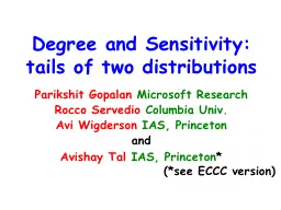
Degree and Sensitivity: tails of two distributions Degree and Sensitivity: tails of two distributions

Degree and Sensitivity: tails of two distributions - PowerPoint Presentation

lois-ondreau
lois-ondreau . @lois-ondreau
Follow
380 views
Uploaded On 2018-02-20

Degree and Sensitivity: tails of two distributions - PPT Presentation

Parikshit Gopalan Microsoft Research Rocco Servedio Columbia Univ Avi Wigderson IAS Princeton and Avishay Tal IAS Princeton see ECCC version Real degree of Boolean functions ID: 633390

sen deg sensitivity conj deg sen conj sensitivity sens fourier tree log degree degε min max real

Share:

Link:

Embed:

Download Presentation from below link

Download Presentation The PPT/PDF document "Degree and Sensitivity: tails of two dis..." is the property of its rightful owner. Permission is granted to download and print the materials on this web site for personal, non-commercial use only, and to display it on your personal computer provided you do not modify the materials and that you retain all copyright notices contained in the materials. By downloading content from our website, you accept the terms of this agreement.


Presentation Transcript

Slide1

Degree and Sensitivity: tails of two distributions

Parikshit

Gopalan

Microsoft Research

Rocco

Servedio

Columbia Univ.

Avi Wigderson

IAS

,

Princeton

and

Avishay

Tal

IAS

,

Princeton

*

(*see ECCC version)Slide2

(Real) degree of Boolean functions

f

: {-1,1

}

n

{-1,1

} in R

[

x

1

,

x

2

,…,

x

n

]

deg

(

f

) = min

d

:

Real polynomial

p

of degree

d

such that

p

(

x

)=

f

(

x

)

x

{

-1,1

}

n

Ex1

:

Maj

(

x

,

y

,

z

) =

½

(

x

+

y

+

z

xyz

)

deg

=3

Ex2

: NAE(

x

,

y

,

z

) =

½

(

xy

+

yz

+

xz

–1

)

deg

=2

p

f

=

unique

multilinear

p

s.t

.

p

(

x

)=

f

(

x

)

x

{-1,1

}

n

p

f

=

T

[

n

]

f’

(

T

)

i

T

x

i

f’

(

T

)

=

Fourier

coefficients

deg

(

f

)

=

deg

(

p

f

) = max |

T

|:

f’

(

T

)

0Slide3

Complexity measures

f

: {-1,1

}

n

 {-1,1}D(f) – Deterministic decision tree complexityR(f) – Probabilistic decision tree complexityQ(f) – Quantum decision tree complexityN(f) – Certificate complexitydeg(f) – Real degreedeg∞(f) – L∞ approximate degreebs(f) – Block sensitivity……[Nisan,…] All parameters are polynomially relatedsen(f) – Sensitivity ??

independent of nSlide4

Sensitivity

f

: {-1,1

}

n

 {-1,1}1-11-111-1-1Gfs(x) = sensitivity of x = vertex degree of x in G

f sen(

f)

=

max

x

s

(

x

)

[Nisan-

Szegedy

]

sen

(

f

) ≤

deg(f)2[Sens-Conjecture] deg(f) ≤ sen(f)c

Understand

G

f

!

!

New parameters

low sensitivity = smooth

Smooth

=

SimpleSlide5

Fourier dist. &

Real approx.

f

: {-1,1

}

n  {-1,1} L2-approximationdegε (f) = min d: ∃ Real polynomial q of degree d such that Ex {-1,1}n [|q(x)-f(x)|2] ≤ ε T f’(T)2 =1 Fourier dist: T [n] with prob

f’(T)2ε

t

=

|

T

|>

t

f’

(

T

)

2

:

Tails

of the Fourier

distribution

deg

ε

(f) = min d: εd ≤ ε - Best approximator q is a truncation of pf - deg0(f) = deg

(

f) Slide6

Main result

f

: {-1,1

}

n

 {-1,1}deg0(f) = deg(f) degε(f) = min d: εd ≤ ε (best approximation in L2)[Sens-Conj] deg0(f) ≤ sen(f)c[Thm1] ε>0 degε (f) ≤ sen(f) log(1/ε)

[Thm2] This is “optimal”:∃c>0,δ

<1 deg

ε

(

f

) ≤

sen

(

f

)

c

log

(1/

ε

)

δ

 [Sens-Conj] Slide7

1

-1

1

-1

1

1-1-1

Sensitive trees

f

: {-1,1

}

n

{-1,1

}

A sensitive tree in

G

f

is a

subgraph

H

of

G

f

H

is a tree

dimensions of edges(H) distinct ts(f) = max {dim H: H

sens

tree}

sen(f) = max

{dim H:

H sens

star}

[Thm3]

deg(f

) ≤ ts(

f)2

[TS-Conj]

deg(f

) ≤ ts

(f)

1

32

1

3

2

3

2Slide8

Moments: Fourier vs. Sensitivity

f

: {-1,1

}

n

 {-1,1}, pf = T f’(T)XT D: draw T [n] with probability f’(T)2Dk=ED[|T|k] : Fourier momentsS: draw x  {-1,1}n uniformly.Sk=Ex[s(x)k]:

Sensitivity moments[Moment-Conj] 

k

D

k

a

k

S

k

(independent of

f

,

n

)

[Fact]

D

1

=

S

1 (Total influence), [Kalai] D2 = S2[Thm4] deg(f) ≤ ts(f)  [Moment-Conj

]

Average-case

variants of deg(

f) & sens(

f)Slide9

Proof of the main result

f

: {-1,1

}

n

 {-1,1}degε(f) = min d: εd ≤ ε (best approximation in L2)[Thm1] ε>0 degε (f) ≤100 sen(f) log(1/ε) s k (t=100sk) εt = |T|>t f’(T)2 = Pr

D[|T|>t] =

PrD[

|

T

|

k

>

t

k

] ≤

≤ E

[

|

T

|

k

]/

t

k

………… ≤ exp(-k) ≤(n/t)k Pr[deg(fρ)

=

k] ≤

(1) (2)

Random restriction

Leaving k var

aliveSlide10

Random restrictions

ρ

:

{

x1,x2,…,xn}  {-1,1,*} at random fromRk= {ρ = (K,y) : K=ρ-1(*), |K|=k, y  {-1,1}n-K }(1) ED[|T|k] ≤ nk Prρ[deg(fρ) = k]Proof:

Prρ [deg(f

ρ) =

k

] =

Pr

[

f’

ρ

(

K

)

≠0]

≥ 2

-2

k

E[

f’

ρ

(

K

)2] Granularity of Fourier = T Prρ [KT] fρ(T)2 Heredity

of

Fourier = (

k/n

)k E

D[|T|

k]Slide11

A switching lemma

(2)

Pr

ρ

[

deg (fρ) = k] ≤ (10sk/n)k(2’) Prρ[ts (fρ) = k] ≤ (10sk/n)kBad = { ρ : ts (fρ) = k }  RkBad  [2n]×[s]k×[2]k ρ  A DFS path in the sensitive tree

|Bad|/|Rk| < (10

sk/n

)

k

[

Moment-

Conj

]

Hastad’s

switching lemma

Has max degree ≤

s

In paper we use

“proper walks”Slide12

Applications

Learning algorithm for low-sensitivity functions in time

(1/

ε

)

poly(s) Under uniform dist: Uses [LMN] Exact learning alg: Uses [GNSTW] New proof of the switching lemmaBetter bounds on Entropy-Influence conj: [EntInf-Conj] Ent(f) ≤ c.Inf(f) [Fact] Ent(f) ≤ c.Inf(f)

.log n

[EntInf-Conj

]

Ent

(

f

) ≤

c

.

Inf

(

f

)

.

log

sen

(

f

)Slide13

Conclusions & open problems

Prove consequences of

[

Sens-

Conj

] [GSTW] degε (f) ≤ sen(f) log(1/ε) [GNSTW] depth(f) ≤ poly(sen(f))Prove [Sens-Conj] !!!If not…deg(f) ≤ ts(f)? Relate new parametersk ED[|T|k] ≤ ak

Ex[s(x)

k] ?

k

E

x

[

s

(

x

)

k

] ≤

b

k

E

D

[|

T

|k] ?