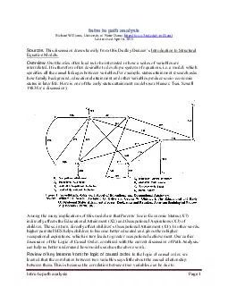
Intro to path analysis Sources This discussion draws heavily from Otis Dudley Duncans - PDF document

Intro to path analysisPage Intro to path analysisRichard Williams, University of Notre Dame, Last revised April 6, 2015 Sources Equation Models. Overview.Our theories often lead us to be interested in how a series of variables are interrelated. Intro to path analysisPage the direct effect of one variable on anotherindirect effects; one variable affects another variable which in turn affects a thirdcommon causes, e.g. X affects both Y and Z.This is spurious associationcorrelated causes, e.g. X is a cause of Z and X is correlated with Yreciprocal causation; each variable is a cause of the otherHence, a correlation can reflect many noncausal influences.Further, a correlation can’t tell you anything about the direction of causality.At the same time, only looking at the direct effect of one variable on another may also not be optimal.Direct effects tell you how a 1 unit change in X will affect Y, holding all other variables constant.However, it may be that other variables are not likely to remain constant if X changes, e.g. a change in X can produce a change in Z which in turn produces a change in Y.Put another way, both the direct and indirect effects of X on Y must be considered if we want to know what effect a change in X will have on Y, i.e. we want to know the total effects(direct + indirect). We have done all this conceptually.Now, we will see how, using path analysis, this is done mathematically and statistically.We will show how the correlation between two variables can be decomposedinto its component parts, i.e. we will show how much of a correlation is due to direct effects, indirect effects, common causes and correlated causesWe will further show how each of the structural effectsin a model affects the correlations in the model. Path analysis terminology.Consider the following diagram: X1X2X3X4 uvw In this diagram,X1 is an exogenous variable.Exogenous variables are those variables whose causes are not explicitly represented in the model.Exogenous variables are causally prior to all dependent variables in the model.There is no causal ordering of the exogenous variables.There can be more than one exogenous variable in a model.For example, if there was a 2headed arrow linking X1 and X2 instead of a 1headed arrow, then X1 and X2 would both be exogenous.Conversely, X2, X3, and X4 are endogenousvariables.The causes of endogenous variables are specified in the modelExogenous variables must always be independent variables.However, endogenous variables can be either dependent or independent.For example, X1 is a cause of X2, but X2 is itself a cause of X3 and X4. Intro to path analysisPage u, v, and w are disturbances, or, if you prefer, the residual terms. Many notations are used for disturbances; indeed, sometimes no notation is used at all, there is just an arrow coming in from out of nowhere., and would also be a good notation, given our past practices.The one way arrows represent the direct causal effects in the model, also known as the structural effectsSometimes, the names for these effects are specifically labeled, but other times they are left implicit.The structural equationsin the above diagram can be written as XXuXXXvXXXXw221133113224411422433 Note that we use 2 subscripts for each structural effect.The first subscript stands for the DV, the second stands for the IV.When there are multiple equations, this kind of notation is necessary to keep things straight.Note, too, that intercepts are not included.Discussions of path analysis are simplified by assuming that all variables are “centered,” i.e. the mean of the variable has been subtracted from each case.Finally, note that the paths linking the disturbances to their respective variables areset equal to 1.In the above example, each DV was affected by all the other predetermined variables, i.e. those variables which are causally prior to it.We refer to such a model as being fully recursive, for reasons we will explain later.There is no requirement that each DV be affected by all the predetermined variables, of course.For example, 43could equal zero, in which case that path would be deleted from the model.Indeed, it is fairly easy to include paths in a model; the theoretically difficult part is deciding which paths to leave out.Determining correlations and coefficients in a path model using standardized variables.We will now start to examine the mathematics behind a path model.For convenience, WE WILL ASSUME THAT ALL VARIABLES HAVE A MEAN OF 0 AND A VARIANCE OF 1, i.e. are standardized.This makes the math easier, and it is easy enough later on to go back to unstandardized variables.Recall that, when variables are standardized,E(X) = V(X) = 1, E(X) = COV(X) = 12(where 12is the population counterpart to the sample estimate r12Also, we assume (at least for now) that the disturbance in an equation is uncorrelated with any of the IVs in the equation. (Note, however, that the disturbance in each equation has a nonzero correlation with the dependent variable in that equation and (in general) with the dependent variable in each “later” equation.)Keeping the above in mind, if we know the structural parameters, it is fairly easy to compute the underlying correlations.Perhaps more importantly, it is possible to decompose the correlation between two variables into the sources of association noted above, e.g. correlation due to direct effects, correlation due to indirect effects, etc.And, of course, if we know the correlations, we can compute the structural parameters, although this is somewhat harder to do by hand.There are a couple of ways of doing this.The normal equations approach is more mathematical; while perhaps less intuitive, it is less prone to mistakes. second, Sewell Wright’s rule, is very Intro to path analysisPage diagramoriented and is perhaps more intuitive to most people once you understand it.I find that using both together is often helpful.(Both approaches are probably best learned via examples, so in class I will probably just skip to the examples and then let you reread the following explanations on your own).Normal equations.To get the normal equations, each structural equation is multiplied by its predetermined variables, and then expectations are taken. If the structural parameters are known, simple algebra then yields the correlations. We’ll show how to use normal equations in the more complicated example.Sewell Wright’s multiplication rule:To find the correlation between Xand X, where Xappears “later”in the model, begin at Xand read backto Xalong each distinct direct and indirect (compound) path, forming the product of the coefficients along that path.(This will give you the correlation between Xand Xthat is due to the direct and indirect effects of XAfter reading back, read forward(if necessary), but only one reversal from back to forward is permitted.(This will give you correlation that is due to common causes.)A doubleheaded arrow may be read either forward or backward, but you can only pass through 1 doubleheaded arrowon each transit.(This will give you correlation due to correlated causes)If you pass through a variable, you may not return to it on that transit.Sum the products obtained for all the linkages between Xand X(The main trick to using Wright’s rule is to make sure you don’t miss any linkages, count linkages twice, or make illegal double reversals.)This will give you the total correlation between the 2 variables.To illustrate path analysis principles, we’ll first go over a generic and complicated example.We’ll then present a fairly simple substantive (albeit hypothetical) example similar to what we’ve discussed before. Generic, Complicated Example(pretty much stolen from Duncan)We will illustrate both the Wright rule and the use of normal equations for each of the 3 structural equations in the modelpresented earlier X1X2X3X4 uvw Intro to path analysisPage (1)X2.For X2, the structural equation is XXu2211 吀桥湬y⁰re摥ter洀i湥搠癡ria扬e⁩s⁘ㄮ䠀敮捥Ⰰ⁩昀眀e畬ti灬y⁢潴栠si摥s昀⁴桥⁡扯癥⁥煵ati潮 戀y⁘ㄠa湤⁴桥渠ta步 e砀灥挀tati潮sⰠ眀e get⁴桥潲洀al⁥煵ati潮 uXEXEXXE NOTE: How did we get from the structural equation to the normal equation?First, we multiplied both sides of the structural equation by X1, and then we took the expectations of both sides, i.e. 2121121212112121211212)()()(uXEXEXXEuXXXXuXX Again, remember that when variables are standardized,E(X) = 1 and E(X) = (where is the population counterpart to the sample estimate rAlso remember that we are assuming that the disturbance in an equation is uncorrelated with any of the IVs in the equation, ergo E(Xu) = 0. Hence, as we have seen before, in a bivariate regression, the correlation is the same as the standardized regression coefficient.Also, all of the correlation between X1 and X2 is causal. X1X2X3X4 uvw SW Rule: Go back from X2 to X1.(2)X3.For X3, the structural equation is XXXv3311322 吀h敲攠慲攠t眀o⁰r敤整敲洀in敤⁶慲i慢l敳Ⰰ 堀1⁡n搀⁘2⸀吀a歩湧 ea挀栠i渠t畲測⁴he潲洀al⁥煵ati潮s⁡re vXEXXEXEXXE (Remember that 2112As the above makes clear, there are two sources of correlation between X1 and X3: Intro to path analysisPage (a)There is a direct effect of X1 on X3 (represented in 31 X1X2X3X4 uvw SW Rule: Go back from X3 to X1.(b)An indirect effect of X1 operating through X2 (reflected by 3221All of the association between X1 and X3 is causal. X1X2X3X4 uvw SW Rule: Go back from X3 to X2, and then back from X2 to X1. NOTE: Recall that the sum of a variable’s direct effect and its indirect effects is known as its total effectSo, in this case, the total effect of X1 on X3 is 213231 䐀潩湧⁴桥⁳a洀e⁴桩湧 昀潲⁘㈠a湤⁘㌬⁷e 来t vXEXEXXEXXE Again, as the above makes clear, there are two sources of correlation between X2 and X3:(a)There is a direct effect of X2 on X3 (represented in 32). X1X2X3X4 uvw SW Rule: Go back from X3 to X2. Intro to path analysisPage (b)But, there is also correlation due to a common cause, X1 (reflected by 31Hence, part of the correlation between X2 and X3 is spurious. X1X2X3X4 uvw SW Rule: Go back from X3 to X1, go forward from X1 to X2.(3)X4.For X4, the predetermined variables are X1, X2, and X3.The structural equation is XXXXw4411422433 吀桥潲洀al⁥煵ati潮s⁡reⰠ昀irstⰠ昀潲⁘ㄬ wXEXXEXXEXEXXE This shows there are 4 sources of association between X1 and X4:(a) Association due to the direct effect of X1 on X4 (41 X1X2X3X4 uvw SW Rule: Go back from X4 to X1. Intro to path analysisPage (b) Association due to indirect effectX1 affectsX2 which then affects X44221 X1X2X3X4 uvw SW Rule: Go back from X4 to X2, go back from X2 to X1.(c) Association due to anotherindirect effectX1 affectsX3 which then affects X44331 X1X2X3X4 uvw SW Rule: Go back from X4 to X3, go back from X3 to X1.(d) Association due to yet anotherindirect effectX1 affectsX2, which then affects X3, which then affects X4 (433221 X1X2X3X4 uvw SW Rule: Go back from X4 toX3, back from X3 to X2, back from X2 to X1.Note that you sum (b), (c) and (d) to get the total indirect effect of X1 on X4.Note too that all of the correlation between X1 and X4 is causal. Intro to path analysisPage The normal equations for X2 and X4 are 213143324342214121313243422141234342124142232432242124142)()()()()()(wXEXXEXEXXEXXE This shows there are 4 sources of association between X2 and X4:(a) Association due to X1 being a common cause of X2 and X4 (4121 X1X2X3X4 uvw SW Rule: GO back from X4 to X1, go forward from X1 to X2.(b) Association due to the direct effect of X2 on X4 (42 X1X2X3X4 uvw SW Rule: Go back from X4 to X2.(c) Association due to the indirect effect of X2 affecting X3 which in turn affects X4 4332 X1X2X3X4 uvw SW Rule: Go back from X4 to X3, go back from X3 to X2. Intro to path analysisPage (d) Associationdue to X1 being a common cause of X2 and X4: X1 directly affects X2 and indirectly affects X4 through X3 (433121 X1X2X3X4 uvw SW Rule: Go back from X4 to X3, back from X3 to X1, forward from X1 to X2.Note that you sum (a) and (d) to get the correlation due to common causes.This represents spurious association, while (b) + (c) represents causal association.The normal equations for X3 and X4 are, 4321314232422132413141432131324221323141432342134143323432342134143)()()()()()()(wXEXEXXEXXEXXE This shows there are 5 sources of association between X3 and X4:(a) Association due to X1 being a common cause of X3 and X4 (4131 X1X2X3X4 uvw SW Rule: Go back from X4 to X1, go forward from X1 to X3. Intro to path analysisPage (b) Association due to X1 being a common cause of X3 (by first affecting X2, which in turn affects X3) and X4 (4121 32 X1X2X3X4 uvw SW rule: Go back from X4 to X1, forward from X1 to X2, forward from X2 to X3.(c) Association due to X2 being a common cause of X3 and X4 (4232 X1X2X3X4 uvw SW Rule: Back from X4 to X2, go forward from X2 to X3.(d)Association due to X1 being a common cause of X3 and X4: X1 directly affects X3 and indirectly affects X4 through X2 (422131 X1X2X3X4 uvw SW Rule: Go back from X4 to X2, back from X2 to X1, forward from X1 to X3. Intro to path analysisPage (e) Association due to X3 being a direct cause of X4 (43 X1X2X3X4 uvw SW Rule: Go back from X4 to X3.Note that you sum (a),(b) (c) and (d) to get the correlation due to common causes.This is the spurious association.There are no indirect effects of X3 on X4. In reviewing the above, note that, if there are no doubleheaded arrows in the model If you go back once and then stop, it is a direct effect If you go back 2 or more times and never come forward, it is an indirect effect If you go back and later come forward, it is correlation due to a common cause Correlated causes.Suppose that, in the above model, X1 and X2 were both exogenous, i.e. there was a doubleheaded arrow between them instead of a 1way arrow.This would not have any significant effect on the math, but it would affect our interpretation of the sources of correlation.Anything involving 12would then have to be interpreted as correlation due to correlated causes.Further, we could not always say what effect changes in X1 would have on other variables, since we wouldn’t know whether changes in X1 would also produce changes in X2 (unless we have good reasons for believing that that couldn’t be the case, e.g. gender and racemight both be exogeneous variables in a model, but we are pretty confidentthat changes in one are not going to produce changes in the other.That is, with twoheaded arrows we often can’t be sure what the indirect effects are, which also means that we can’t be sure what the total effects are.Ergo, he fewer 2headed arrows in a model, the more powerful the model is in terms of the statements it makes.For example: X1X2X3X4 vw Instead of X1 and X3 being correlated because of the indirect effect of X1 affecting X2 which in turn affects X3 (which is a causal relationship) X1 and X3 are correlated because of the Intro to path analysisPage correlated causes of X1 and X2 (which we do not assume to be causal), i.e. X1 is correlated with a cause of X3.Or, X1X2X3X4 vw Instead of X2 and X3 being correlated because they share a common cause, they are correlated because of a correlated cause, i.e. X1 is a cause of X3 and X2 is correlated with X1. SUBSTANTIVE HYPOTHETICALEXAMPLE(Adapted From the 1995 Soc 593 Exam 2):A demographer believes that the following model describes the relationship between Income, Health of the Mother, Use of Infant formula, and Infant deaths.All variables are in standardized form.The hypothesized value of each path is included in the diagram. IncomeMother's HealthInfant Formula UsageInfant Deaths uvw .7-.8-.5-.8 Write out the structural equation for each endogenous variable. IncomeIncomeInc 䐀整敲洀in攠th攠捯洀pl整攠捯rr敬慴ion慴ri砀⸀
刀敭敭戀敲Ⰰ⁶ari慢l敳⁡r攠a湤ar摩稀e搮夀潵⁣a渠畳e⁥it桥r潲洀al⁥煵ati潮sr⁓e眀ell⁗rig桴Ⱐ扵t yo甠洀ig桴⁷a湴⁴漠畳e 扯t栠as⁡⁤潵扬e捨散欀⸀⤀ Intro to path analysisPage Correlation Sewell - Wright Approach r mh,inc = .7 Go back from Mother’s health to Income. (Direct effect of Income on MH) r if,MH = - .8 Go back from IF to MH. (Direct effect of MH on IF) r IF,Inc = - .8 * .7 = - .56 Go back from IF to MH, then back from MH to income. (Indirect effect of Income Income affects mother’s health which in turn affects Infant formula usage) r id,IF = - .5 + - .8* - .8 = .14 Go back from ID to IF. (Direct effect of Infant formula on infant deaths) Then, go back from ID to MH, then go forward from MH to IF.(Mother’s health is a common cause of both Infant formula usage and infant deaths)Note that, even though the direct effect of infant formula usage on infant deaths is negative (which means that using formula reduces infant deaths) the correlation between infant formula usage and infant deaths is positive (which means that those who use formula are more likely to experience infant deaths).We discuss this further below. r id,MH = - .8 + - .8* - .5 = - .4 Go back from ID to MH. (Direct effect of Mother’s Health on Infant deaths) Then, go back from ID to IF to MH. (Indirect effect of Mother’s health on infant deaths Mother’s health affects infant formula usage which in turn affects infant deaths) r id,INC = - .8*.7 + - .5* - .8*.7 .28 Go back from Infant Death to Mother’s Health, then back to Income.(Income is an indirect cause of Infant deaths Income affects mother’s health which in turn affects infant deaths.) Then go back from Infant deaths, then back to Mother’s Health, then back to Income.(Income is yet again an indirect cause Income affects Mother’s Health, which affects Infant Formula Usage, which affects Infant Deaths.) Intro to path analysisPage Decompose the correlation between Infant deaths and Usage of Infant formula intoCorrelation due to direct effects.5 (see path from IF to ID)Correlation due to common causes.8 * .8 = .64 (Mother’s health is a cause of both IF and ID)Suppose the above model is correct, but instead the researcher believed in and estimated the following model: Infant Formula UsageInfant Deaths What conclusions would the researcher likely draw?Why would he make these mistakes?Discuss the consequences of this misspecification.The correlation between IF and ID is positive, hence, if the above model was estimated, the expected value of the coefficient would be .14.This would imply that infant formula usage increases infant deaths, when in reality the correct model shows that it decreases them.The correlation is positive because of the common cause of Mother’s health: less healthy mothers are more likely to use infant formula, and they are also more likely to have higher infant death rates.Belief in the above model could lead to a reduction in infant formula usage, which would have exactly the opposite effect of what was intended. Intro to path analysisPage Appendix: Basic Path Analysiswith StataWe have been doing things a bit backwards here. We have been starting with the coefficients, and then figured out what the correlations must be. Normally, of course, we start with the data/correlations and then estimate the coefficients. Nonetheless, we can use Stata to verify we have calculated the correlations correctly.Just give Stata the correlations we computed by hand and then use one of the methods below to estimate thevarious regressions.If we’ve done everything right, the regression parameters should come out the same as in the path diagram.Remember, this is easier if you use the “input matrix by hand” submenu.lick Data/ Matrices / Input matrix by hand.) There are now at least three ways to estimate the path models (or at least, the simplemodels we are estimating here; approach 2, the semcommands, is probably best for more complicated models.)I. Estimate separate regressions for each dependent variable. Intro to path analysisPage &#x/MCI; 11;&#x 000;&#x/MCI; 11;&#x 000;-------------+---------------------------------------------------------------- &#x/MCI; 12;&#x 000;&#x/MCI; 12;&#x 000; income | 1.63e-09 .1237684 0.00 1.000 -.2456784 .2456784 &#x/MCI; 13;&#x 000;&#x/MCI; 13;&#x 000; mhealth | -.8 .1709021 -4.68 0.000 -1.139238 -.4607621 &#x/MCI; 14;&#x 000;&#x/MCI; 14;&#x 000; formula | -.5 .1473139 -3.39 0.001 -.7924158 -.2075842 &#x/MCI; 15;&#x 000;&#x/MCI; 15;&#x 000; _cons | -6.54e-09 .0879453 -0.00 1.000 -.17457 .17457 &#x/MCI; 16;&#x 000;&#x/MCI; 16;&#x 000;------------------------------------------------------------------------------ &#x/MCI; 17;&#x 000;&#x/MCI; 17;&#x 000; &#x/MCI; 18;&#x 000;&#x/MCI; 18;&#x 000;. * The mis-specified model &#x/MCI; 19;&#x 000;&#x/MCI; 19;&#x 000;. reg death formula &#x/MCI; 20;&#x 000;&#x/MCI; 20;&#x 000; &#x/MCI; 21;&#x 000;&#x/MCI; 21;&#x 000; Source | SS df MS Number of obs = 100 &#x/MCI; 22;&#x 000;&#x/MCI; 22;&#x 000;-------------+------------------------------ F( 1, 98) = 1.96 &#x/MCI; 23;&#x 000;&#x/MCI; 23;&#x 000; &#x/MCI; 23;&#x 000;Model | 1.94039993 1 1.94039993 Prob F = 0.1648 &#x/MCI; 24;&#x 000;&#x/MCI; 24;&#x 000; Residual | 97.0596001 98 .990404083 R-squared = 0.0196 &#x/MCI; 25;&#x 000;&#x/MCI; 25;&#x 000;-------------+------------------------------ Adj R-squared = 0.0096 &#x/MCI; 26;&#x 000;&#x/MCI; 26;&#x 000; Total | 99.0000001 99 1 Root MSE = .99519 &#x/MCI; 27;&#x 000;&#x/MCI; 27;&#x 000; &#x/MCI; 28;&#x 000;&#x/MCI; 28;&#x 000;------------------------------------------------------------------------------ &#x/MCI; 29;&#x 000;&#x/MCI; 29;&#x 000; &#x/MCI; 29;&#x 000;death | Coef. Std. Err. t P|t| [95% Conf. Interval] &#x/MCI; 30;&#x 000;&#x/MCI; 30;&#x 000;-------------+---------------------------------------------------------------- &#x/MCI; 31;&#x 000;&#x/MCI; 31;&#x 000; formula | .14 .1000204 1.40 0.165 -.0584872 .3384872 &#x/MCI; 32;&#x 000;&#x/MCI; 32;&#x 000; _cons | -5.23e-09 .099519 -0.00 1.000 -.1974923 .1974923 &#x/MCI; 33;&#x 000;&#x/MCI; 33;&#x 000;------------------------------------------------------------------------------ &#x/MCI; 34;&#x 000;&#x/MCI; 34;&#x 000; &#x/MCI; 35;&#x 000;&#x/MCI; 35;&#x 000;II. The sem commandWe can also use the sem(Structural Equation Modeling) commands that were introduced in Stata 11. This example is pretty simple so it isn’t too hard to do. Among the nice features of sem is that you can specify all the equations at once, and you can get estimates of the direct, indirect and total effectsTime permitting, we will talk about more later in the semester. Intro to path analysisPage ------------------------------------------------------------------------------ ------------- ------------- ------------------------------------------------------------------------------ . * Estimate the direct, indirect, and total effects of each variable. estat teffects Direct effec------------------------------------------------------------------------------ ------------- Intro to path analysisPage Indirect effects------------------------------------------------------------------------------ Structural | ---------------------------- ------------- ----------------------------------- . * Incorrect model. sem death Endogenous variables Observed: death Exogenous variables Fitting target model: Iteration 0: log likelihood = Iteration 1: lo Structural equation model Number of obs = 100Estimation method = ml Intro to path analysisPage &#x/MCI; 3 ;&#x/MCI; 3 ;-------------+---------------------------------------------------------------- &#x/MCI; 4 ;&#x/MCI; 4 ;Structural | &#x/MCI; 5 ;&#x/MCI; 5 ; death - | &#x/MCI; 6 ;&#x/MCI; 6 ; formula | .14 .0990152 1.41 0.157 -.0540661 .3340661 &#x/MCI; 7 ;&#x/MCI; 7 ; _cons | -5.23e-09 .0985188 -0.00 1.000 -.1930934 .1930934 &#x/MCI; 8 ;&#x/MCI; 8 ;-------------+---------------------------------------------------------------- &#x/MCI; 9 ;&#x/MCI; 9 ;Variance | &#x/MCI; 10;&#x 000;&#x/MCI; 10;&#x 000; e.death | .970596 .137263 .7356317 1.280609 &#x/MCI; 11;&#x 000;&#x/MCI; 11;&#x 000;------------------------------------------------------------------------------ &#x/MCI; 12;&#x 000;&#x/MCI; 12;&#x 000;&#x/MCI; 12;&#x 000;LR test of model vs. saturated: chi2(0) = 0.00, Prob chi2 = . &#x/MCI; 13;&#x 000;&#x/MCI; 13;&#x 000; &#x/MCI; 14;&#x 000;&#x/MCI; 14;&#x 000;III. UCLA’s pathreg commandYou can get this with the command.Again, it lets you specify all the equations at once, but doesn’t offer the many additional features that does. Also, does not support factor variables as of March 2013.