PDF-Evaluating the Effectof RoadHump on Traffic Volume and Noise Level at

Author : pamella-moone | Published Date : 2016-06-13

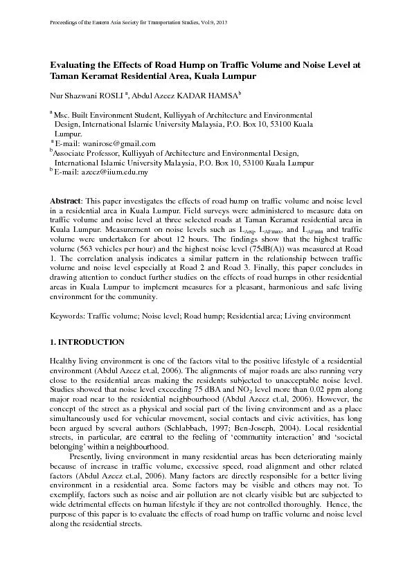
Nur Shazwani ROSLI Abdul Azeez KADAR HAMSA Msc Built Environment Student Kulliyyah of Architecture and Environmental Design International Islamic Unive mail azeeziiumedumy

Presentation Embed Code

<iframe width="560" height="315" src="https://www.docslides.com/embed/359966" frameborder="0" allowfullscreen></iframe>

Download Presentation

Download Presentation The PPT/PDF document "Evaluating the Effectof RoadHump on Traf..." is the property of its rightful owner. Permission is granted to download and print the materials on this website for personal, non-commercial use only, and to display it on your personal computer provided you do not modify the materials and that you retain all copyright notices contained in the materials. By downloading content from our website, you accept the terms of this agreement.

Evaluating the Effectof RoadHump on Traffic Volume and Noise Level at: Transcript

Download Document

Here is the link to download the presentation.
"Evaluating the Effectof RoadHump on Traffic Volume and Noise Level at"The content belongs to its owner. You may download and print it for personal use, without modification, and keep all copyright notices. By downloading, you agree to these terms.