/
Chapter 5 A Closer Look at Instruction Set Architectures Chapter 5 A Closer Look at Instruction Set Architectures

Chapter 5 A Closer Look at Instruction Set Architectures - PowerPoint Presentation

pasty-toler
pasty-toler . @pasty-toler
Follow
369 views
Uploaded On 2018-09-21

Chapter 5 A Closer Look at Instruction Set Architectures - PPT Presentation

2 Chapter 5 Objectives Understand the factors involved in instruction set architecture design Gain familiarity with memory addressing modes Understand the concepts of instructionlevel pipelining and its affect upon execution performance ID: 673387

formats instruction addressing address instruction formats address addressing instructions operands pipeline memory stack register architecture operand bit store expression

Share:

Link:

Embed:

Download Presentation from below link

Download Presentation The PPT/PDF document "Chapter 5 A Closer Look at Instruction S..." is the property of its rightful owner. Permission is granted to download and print the materials on this web site for personal, non-commercial use only, and to display it on your personal computer provided you do not modify the materials and that you retain all copyright notices contained in the materials. By downloading content from our website, you accept the terms of this agreement.


Presentation Transcript

Slide1

Chapter 5

A Closer Look at Instruction Set ArchitecturesSlide2

2

Chapter 5 Objectives

Understand the factors involved in instruction set architecture design.

Gain familiarity with memory addressing modes.

Understand the concepts of instruction-level pipelining and its affect upon execution performance.Slide3

3

5.1 Introduction

This chapter builds upon the ideas in Chapter 4

.

We present a detailed look at different instruction formats, operand types, and memory access methods.

We will see the interrelation between machine organization and instruction formats.

This leads to a deeper understanding of computer architecture in general.Slide4

4

5.2 Instruction Formats

Instruction sets are differentiated by the following:

Number of bits per instruction.

Stack-based or register-based.

Number of explicit operands per instruction.

Operand location.

Types of operations.

Type and size of operands.Slide5

5

5.2 Instruction Formats

Instruction set architectures are measured according to:

Main memory space occupied by a program.

Instruction complexity.

Instruction length (in bits).

Total number of instructions in the instruction set.Slide6

6

5.2 Instruction Formats

In designing an instruction set, consideration is given to:

Instruction length.

Whether short, long, or variable.

Number of operands.

Number of addressable registers.

Memory organization.

Whether byte- or word addressable.

Addressing modes.

Choose any or all: direct, indirect or indexed.Slide7

7

Byte ordering, or

endianness

, is another major architectural consideration.

If we have a two-byte integer, the integer may be stored so that the least significant byte is followed by the most significant byte or vice versa.

In

little endian

machines,

the least significant byte is followed by the most significant byte.

Big endian

machines store the most significant byte first (at the lower address).

5.2 Instruction FormatsSlide8

8

As an example, suppose we have the hexadecimal number

0x12345678

.

The big endian and small endian arrangements of the bytes are shown below.

5.2 Instruction FormatsSlide9

9

A larger example: A computer uses 32-bit integers. The values 0xABCD1234, 0x00FE4321, and 0x10 would be stored sequentially in memory, starting at address 0x200 as below.

5.2 Instruction FormatsSlide10

10

5.2 Instruction Formats

Big endian:

Is more natural.

The sign of the number can be determined by looking at the byte at address offset 0.

Strings and integers are stored in the same order.

Little endian:

Makes it easier to place values on non-word boundaries.

Conversion from a 16-bit integer address to a 32-bit integer address does not require any arithmetic.Slide11

11

5.2 Instruction Formats

The next consideration for architecture design concerns how the CPU will store data.

We have three choices:

1. A stack architecture

2. An accumulator architecture

3. A general purpose register architecture.

In choosing one over the other, the tradeoffs are simplicity (and cost) of hardware design with execution speed and ease of use.Slide12

12

5.2 Instruction Formats

In a stack architecture, instructions and operands are implicitly taken from the stack.

A stack cannot be accessed randomly.

In an accumulator architecture, one operand of a binary operation is implicitly in the accumulator.

One operand is in memory, creating lots of bus traffic

.

In a general purpose register (GPR) architecture, registers can be used instead of memory.

Faster than accumulator architecture.

Efficient implementation for compilers.

Results in longer instructions.Slide13

13

5.2 Instruction Formats

Most systems today are GPR systems.

There are three types:

Memory-memory where two or three operands may be in memory.

Register-memory where at least one operand must be in a register.

Load-store where no operands may be in memory.

The number of operands and the number of available registers has a direct affect on instruction length.Slide14

14

5.2 Instruction Formats

Stack machines use one

- and zero-operand instructions.

LOAD

and

STORE

instructions require a single memory address operand.

Other instructions use operands from the stack implicitly.

PUSH

and

POP

operations involve only the stack’s top element.

Binary instructions (e.g.,

ADD

,

MULT

) use the top two items on the stack.Slide15

15

5.2 Instruction Formats

Stack architectures require us to think about arithmetic expressions a little differently.

We are accustomed to writing expressions using

infix

notation, such as: Z = X + Y.

Stack arithmetic requires that we use

postfix

notation: Z = XY+.

This is also called

reverse Polish notation

, (somewhat) in honor of its Polish inventor, Jan Lukasiewicz (1878 - 1956).Slide16

16

5.2 Instruction Formats

The principal advantage of postfix notation is that parentheses are not used.

For example, the infix expression,

Z = (X

Y) + (W

U),

becomes:

Z = X Y

W U

+

in postfix notation.Slide17

17

5.2 Instruction Formats

Example: Convert the infix expression (2+3) - 6/3 to postfix:

The sum 2 + 3 in parentheses takes precedence; we replace the term with

2 3 +.

2 3+ - 6/3 Slide18

18

5.2 Instruction Formats

Example: Convert the infix expression (2+3) - 6/3 to postfix:

The division operator takes next precedence; we replace 6/3 with

6 3 /.

2 3+ - 6 3/ Slide19

19

5.2 Instruction Formats

Example: Convert the infix expression (2+3) - 6/3 to postfix:

The quotient 6/3 is subtracted from the sum of 2 + 3, so we move the - operator to the end.

2 3+ 6 3/ - Slide20

20

5.2 Instruction Formats

Example: Use a stack to evaluate the postfix expression 2 3 + 6 3 / - :

Scanning the expression from left to right, push operands onto the stack, until an operator is found

6

2

3

3

+

-

/

3

2 Slide21

21

5.2 Instruction Formats

Example: Use a stack to evaluate the postfix expression 2 3 + 6 3 / - :

Pop the two operands and carry out the operation indicated by the operator. Push the result back on the stack.

6

5

3

+

-

/

3

2 Slide22

22

5.2 Instruction Formats

Example: Use a stack to evaluate the postfix expression 2 3 + 6 3 / - :

Push operands until another operator is found.

6

5

3

+

-

/

3

2

3

6 Slide23

23

5.2 Instruction Formats

Example: Use a stack to evaluate the postfix expression 2 3 + 6 3 / - :

Carry out the operation and push the result.

6

5

3

+

-

/

3

2

2 Slide24

24

5.2 Instruction Formats

Example: Use a stack to evaluate the postfix expression 2 3 + 6 3 / - :

Finding another operator, carry out the operation and push the result.

The answer is at the top of the stack.

6

3

3

+

-

/

3

2 Slide25

25

5.2 Instruction Formats

Let's see how to evaluate an infix expression using different instruction formats.

With a three-address ISA, (e.g.,mainframes), the infix expression,

Z = X

Y + W

U

might look like this:

MULT R1,X,Y

MULT R2,W,U

ADD Z,R1,R2Slide26

26

5.2 Instruction Formats

In a two-address ISA, (e.g.,Intel, Motorola), the infix expression,

Z = X

Y + W

U

might look like this:

LOAD R1,X

MULT R1,Y

LOAD R2,W

MULT R2,U

ADD R1,R2

STORE Z,R1

Note: One-address ISAs usually require one operand to be a register.Slide27

27

5.2 Instruction Formats

In a one-address ISA, like MARIE, the infix expression,

Z = X

Y + W

U

looks like this:

LOAD X

MULT Y

STORE TEMP

LOAD W

MULT U

ADD TEMP

STORE ZSlide28

28

5.2 Instruction Formats

In a stack ISA, the postfix expression,

Z = X Y

W U

+

might look like this:

PUSH X

PUSH Y

MULT

PUSH W

PUSH U

MULT

ADD

PUSH Z

Would this program require more execution time than the corresponding (shorter) program that we saw in the 3-address ISA?Slide29

29

5.2 Instruction Formats

We have seen how instruction length is affected by the number of operands supported by the ISA.

In any instruction set, not all instructions require the same number of operands.

Operations that require no operands, such as

HALT

, necessarily waste some space when fixed-length instructions are used.

One way to recover some of this space is to use expanding opcodes.Slide30

30

5.2 Instruction Formats

A system has 16 registers and 4K of memory.

We need 4 bits to access one of the registers. We also need 12 bits for a memory address.

If the system is to have 16-bit instructions, we have two choices for our instructions:Slide31

31

5.2 Instruction Formats

If we allow the length of the

opcode

to vary, we could create a very rich instruction set:Slide32

32

5.2 Instruction Formats

Example: Given 8-bit instructions, is it possible to allow the following to be encoded?

3 instructions with two 3-bit operands.

2 instructions with one 4-bit operand.

4 instructions with one 3-bit operand.

3

2

3

= 192 bits for the 3-bit operands

2

2

4

= 32 bits for the 4-bit operands

4

2

3

= 32 bits for the 3-bit operands.

We need:

Total: 256 bits.Slide33

33

5.2 Instruction Formats

With a total of 256 bits required, we can exactly encode our instruction set in 8 bits!

3

2

3

= 192 bits for the 3-bit operands

2

2

4

= 32 bits for the 4-bit operands

4

2

3

= 32 bits for the 3-bit operands.

We need:

Total: 256 bits.

One such encoding is shown on the next slide.Slide34

34

5.2 Instruction FormatsSlide35

35

5.3 Instruction types

Instructions fall into several broad categories that you should be familiar with:

Data movement.

Arithmetic.

Boolean.

Bit manipulation.

I/O.

Control transfer.

Special purpose.

Can you think of some examples of each of these?Slide36

36

5.4 Addressing

Addressing modes specify where an operand is located.

They can specify a constant, a register, or a memory location.

The actual location of an operand is its

effective address

.

Certain addressing modes allow us to determine the address of an operand dynamically.Slide37

37

5.4 Addressing

Immediate addressing

is where the data is part of the instruction.

Direct addressing

is where the address of the data is given in the instruction.

Register addressing

is where the data is located in a register.

Indirect addressing

gives the address of the address of the data in the instruction.

Register indirect addressing

uses a register to store the address of the address of the data.Slide38

38

5.4 Addressing

Indexed addressing

uses a register (implicitly or explicitly) as an offset, which is added to the address in the operand to determine the effective address of the data.

Based addressing

is similar except that a base register is used instead of an index register.

The difference between these two is that an index register holds an offset relative to the address given in the instruction, a base register holds a base address where the address field represents a displacement from this base.Slide39

39

5.4 Addressing

In

stack addressing

the operand is assumed to be on top of the stack.

There are many variations to these addressing modes including:

Indirect indexed.

Base/offset.

Self-relative

Auto increment - decrement.

We won’t cover these in detail.

Let’s look at an example of the principal addressing modes.Slide40

40

5.4 Addressing

For the instruction shown, what value is loaded into the accumulator for each addressing mode?Slide41

41

5.4 Addressing

For the instruction shown, what value is loaded into the accumulator for each addressing mode?Slide42

42

5.5 Instruction Pipelining

Some CPUs divide the fetch-decode-execute cycle into smaller steps.

These smaller steps can often be executed in parallel to increase throughput.

Such parallel execution is called

instruction pipelining

.

Instruction pipelining provides for

instruction level parallelism

(

ILP

)

The next slide shows an example of instruction pipelining.Slide43

43

Suppose a fetch-decode-execute cycle were broken into the following smaller steps:

Suppose we have a six-stage pipeline. S1 fetches the instruction, S2 decodes it, S3 determines the address of the operands, S4 fetches them, S5 executes the instruction, and S6 stores the result.

1. Fetch instruction. 4. Fetch operands.

2. Decode opcode. 5. Execute instruction.

3. Calculate effective 6. Store result.

address of operands.

5.5 Instruction PipeliningSlide44

44

5.5 Instruction Pipelining

For every clock cycle, one small step is carried out, and the stages are overlapped.

S1. Fetch instruction. S4. Fetch operands.

S2. Decode opcode. S5. Execute.

S3. Calculate effective S6. Store result.

address of operands.Slide45

45

5.5 Instruction Pipelining

The theoretical speedup offered by a pipeline can be determined as follows:

Let

t

p

be the time per stage. Each instruction represents a task,

T

, in the pipeline.

The first task (instruction) requires

k

t

p

time to complete in a

k

-stage pipeline. The remaining (

n

- 1) tasks emerge from the pipeline one per cycle. So the total time to complete the remaining tasks is (

n

- 1)

t

p

.

Thus, to complete

n

tasks using a

k

-stage pipeline requires:

(

k

t

p

) + (

n

- 1)

t

p

= (

k

+

n

- 1)

t

p

.Slide46

46

5.5 Instruction Pipelining

If we take the time required to complete

n

tasks without a pipeline and divide it by the time it takes to complete

n

tasks using a pipeline, we find:

If we take the limit as

n

approaches infinity, (

k

+

n

- 1) approaches

n,

which results in a theoretical speedup of:Slide47

47

5.5 Instruction Pipelining

Our neat equations take a number of things for granted.

First, we have to assume that the architecture supports fetching instructions and data in parallel.

Second, we assume that the pipeline can be kept filled at all times. This is not always the case. Pipeline

hazards

arise that cause pipeline conflicts and stalls.Slide48

48

5.5 Instruction Pipelining

An instruction pipeline may stall, or be flushed for any of the following reasons:

Resource conflicts.

Data dependencies.

Conditional branching.

Measures can be taken at the software level as well as at the hardware level to reduce the effects of these hazards, but they cannot be totally eliminated.Slide49

49

5.6

Real-World Examples of ISAs

We return briefly to the Intel and MIPS architectures from the last chapter, using some of the ideas introduced in this chapter.

Intel introduced pipelining to their processor line with its Pentium chip.

The first Pentium had two five-stage pipelines. Each subsequent Pentium processor had a longer pipeline than its predecessor with the Pentium IV having a 24-stage pipeline.

The Itanium (IA-64) has only a 10-stage pipeline.Slide50

50

5.6

Real-World Examples of ISAs

Intel processors support a wide array of addressing modes.

The original 8086 provided 17 ways to address memory, most of them variants on the methods presented in this chapter.

Owing to their need for backward compatibility, the Pentium chips also support these 17 addressing modes.

The Itanium, having a RISC core, supports only one: register indirect addressing with optional post increment.Slide51

51

5.6

Real-World Examples of ISAs

MIPS was an acronym for

Microprocessor Without Interlocked Pipeline Stages

.

The architecture is little endian and word-addressable with three-address, fixed-length instructions.

Like Intel, the pipeline size of the MIPS processors has grown: The R2000 and R3000 have five-stage pipelines.; the R4000 and R4400 have 8-stage pipelines.Slide52

52

5.6

Real-World Examples of ISAs

The R10000 has three pipelines: A five-stage pipeline for integer instructions, a seven-stage pipeline for floating-point instructions, and a six-state pipeline for

LOAD/STORE

instructions.

In all MIPS ISAs, only the

LOAD

and

STORE

instructions can access memory.

The ISA uses only base addressing mode.

The assembler accommodates programmers who need to use immediate, register, direct, indirect register, base, or indexed addressing modes.Slide53

53

5.6

Real-World Examples of ISAs

The Java programming language is an interpreted language that runs in a software machine called the

Java Virtual Machine

(JVM).

A JVM is written in a native language for a wide array of processors, including MIPS and Intel.

Like a real machine, the JVM has an ISA all of its own, called

bytecode

. This ISA was designed to be compatible with the architecture of any machine on which the JVM is running.

The next slide shows how the pieces fit together.Slide54

54

5.6

Real-World Examples of ISAsSlide55

55

5.6

Real-World Examples of ISAs

Java

bytecode

is a stack-based language.

Most instructions are zero address instructions.

The JVM has four registers that provide access to five regions of main memory.

All references to memory are offsets from these registers. Java uses no pointers or absolute memory references.

Java was designed for platform interoperability, not performance!Slide56

56

5.6

Real-World Examples of ISAs

Y

ou may not have heard of ARM but most likely use an ARM

processor every day. It is the most widely used 32-bit instruction architecture:

95%+ of smartphones,

80%+ of digital cameras

40%+ of all digital television sets

Founded in 1990, by Apple and others, ARM (Advanced RISC Machine) is now a British firm, ARM Holdings.

ARM Holdings does not manufacture these processors; it sells licenses to manufacture.Slide57

57

5.6

Real-World Examples of ISAs

ARM is a load/store architecture : all data processing must be performed on values in registers, not in memory.

It uses fixed-length, three-operand instructions and simple addressing modes

ARM processors have a minimum of a three-stage pipeline (consisting of fetch, decode, and execute);

Newer

ARM processors

have deeper pipelines (more stages). Some ARM8 implementations have 13-stage integer pipelinesSlide58

58

5.6

Real-World Examples of ISAs

ARM has 37 total registers but their visibility depends on the processor mode.

ARM allows multiple register transfers.

It can simultaneously load or store any subset of the16 general-purpose registers from/to sequential memory addresses.

Control flow instructions include unconditional and conditional branching and procedure calls

Most ARM instructions execute in a single cycle, provided there are no pipeline hazards or memory accesses.Slide59

59

ISAs are distinguished according to their bits per instruction, number of operands per instruction, operand location and types and sizes of operands.

Endianness as another major architectural consideration.

CPU can store store data based on

1. A stack architecture

2. An accumulator architecture

3. A general purpose register architecture

.

Chapter 5 ConclusionSlide60

60

Instructions can be fixed length or variable length.

To enrich the instruction set for a fixed length instruction set, expanding opcodes can be used.

The addressing mode of an ISA is also another important factor. We looked at:

Immediate – Direct

Register – Register Indirect

Indirect – Indexed

Based – Stack

Chapter 5 ConclusionSlide61

61

A

k

-stage pipeline can theoretically produce execution speedup of

k

as compared to a non-pipelined machine.

Pipeline hazards such as resource conflicts and conditional branching prevents this speedup from being achieved in practice.

The Intel, MIPS,

JVM, and ARM

architectures provide good examples of the concepts presented in this chapter.

Chapter 5 Conclusion