PPT-Auto-Regressive HMM PowerPoint Presentation

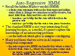
Recall the hidden Markov model HMM a finite state automata with nodes that represent hidden states that is things we cannot necessarily observe but must infer from

Upload by sherrill-nordquist
Published on 2016-11-01

Presentation Embed Code

<iframe width="560" height="315" src="https://www.docslides.com/embed/483088" frameborder="0" allowfullscreen></iframe>

Download Presentation

Download Presentation The PPT/PDF document "Auto-Regressive HMM" is the property of its rightful owner. Permission is granted to download and print the materials on this web site for personal, non-commercial use only, and to display it on your personal computer provided you do not modify the materials and that you retain all copyright notices contained in the materials. By downloading content from our website, you accept the terms of this agreement.