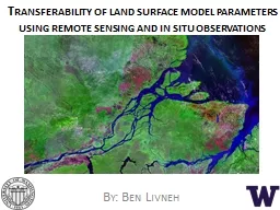
By Ben Livneh Overview Unified Land Model ULM was developed 1 Rigorous calibrations performed at 220 basins 2 Regionalizetransfer calibrated parameters Domain and catchment attribute data sets ID: 648470
Download Presentation The PPT/PDF document "Transferability of land surface model pa..." is the property of its rightful owner. Permission is granted to download and print the materials on this web site for personal, non-commercial use only, and to display it on your personal computer provided you do not modify the materials and that you retain all copyright notices contained in the materials. By downloading content from our website, you accept the terms of this agreement.
Slide1
Transferability of land surface model parameters using remote sensing and in situ observations
By: Ben
LivnehSlide2
Overview
Unified Land Model (ULM) was developed1Rigorous calibrations performed at 220 basins2Regionalize/transfer calibrated parameters
Domain and catchment attribute data setsExperimental set-upResultsConclusions
1.
Livneh et al. 2011; 2.
Livneh
et al., 2012Slide3
Unified Land Model (ULM) Regionalization
Goal: establish a predictive relationship between ULM parameters,
Θ, and observable catchment features, η (e.g.
θ= a + bη) for a new model, ULM.Motivation: extend recent model calibrations to new
domains; calibration
is often
impractical/impossible.
3
ULM field capacity parameter
θ
η
Greenness Fraction (satellite)Slide4
Experimental domain and predictands,
Θ220 MOPEX
1 basins, spanning a wide range of hydro-climatologyCalibrated model parameters, Θ, for each basin were obtained from a recent study
2 as inputs to the regionalization procedure (predictands).
1.
Schaake
et al., 2006; 2.
Livneh
et al., 2012Slide5
Summary of candidate catchment attributes,
η
Meteorological attributes
Description
Quantity
Precipitation, Temperature, Wind – monthly, seasonal, annual means, standard deviations, minima, and maxima
Derived from station co-op data and reanalysis fields (wind
only)
1
16
Geomorphic attributes
Basin area, mean elevation, maximum relief, approx. length of main stream, relief ratio, shape factor, length-to-width ratio, elongation ratio
Defined from DEM and USGS GIS HUC 250K
database
2
8
Land surface characteristic attributes
Percentage of basin covered in forest; Satellite-based greenness fraction and albedo – monthly, seasonal, annual means, standard deviations, minimums, and maximums
Required as inputs into
ULM
3
22
Soil texture attributes
Tension and free water storages, hydraulic conductivities, impervious areas, percolation constant, recession slope.Sacramento model a priori values from soil texture relationship413Remote sensing attributesEvapotranspiration – monthly, seasonal, annual means, standard deviations, minima, and maximaDerived entirely from satellite data (MODIS, SRB)58TWSC – monthly, seasonal, annual means, standard deviations, minima, and maximaGRACE data, mean of 3 processing streams68GAGES-II attributesSoils data, climatic, land-use, morphology transitionary data, population density, drainage density classes, and anthropogenic disturbance factorsA single basin-average value for each field, only floating point data considered (i.e. no integer class data)7313
Total: 388
1.
Livneh et al. 2012b; 2.
Seaber
et al. 1987; 2.
Gutman
and
Ivanov
, 1998; 4.
Koren
et al. 2003; 5. Tang et al. 2009; 6. Swenson and
Wahr
, 2006, Falcone et al. 2010 Slide6
Regionalization methodology
Step-wise principal components regression (PCR) procedure1,2 was selected to maximize explanatory
skill and minimize potential redundancy/inter-correlation. Jack-knifing validation chosen.
θ1=a+b1η1+b
2
η
2
+…+
b
n
η
n
Additional experiment:
resample calibrated model parameters prior to developing the equation, based on their zonal representativeness, i.e. Zonalization
θ’1=c+d1
η1+d2η2+…+
dnηn1. Garen, 1992; 2. Rosenberg et al. 2011
θ1-LOCAL=θ1-ZONAL=
“classic” regionalizationSlide7
Zonalization
procedure
10 calibrated parameter sets per basin1
that are Pareto-optimal, ΘP, i.e. non-dominant multiple-objective functions: streamflow correlation
,
R
, diff. in means
,
α
,
diff in std. deviations
,
β
.Compute an additional objective function Nash-Sutcliffe Efficiency2, NSE (-∞,1)Exp 1: Select local optimum: based on highest NSE
Θ
P1
ΘP2ΘP3ΘP4
ΘP5ΘP6ΘP7
Θ
P8
Θ
P9
Θ
P10
Highest NSE
Lowest NSElocal optimum ΘP,LOCAL = ΘP1Local performance ranking1. Livneh et al. 2012a; Nash and Sutcliffe, 1970θi-LOCAL=a+b1η1+b2η2+…+bnηnSlide8
Zonalization
procedure
10 calibrated parameter sets
per basin1 that are Pareto-optimal, ΘP
, i.e. non-dominant multiple-objective functions: streamflow
correlation
,
R
, diff. in means
,
α
,
diff in std. deviations
, β.Compute an additional objective function Nash-Sutcliffe Efficiency (NSE)Exp 1: Select local optimum: based on highest NSE
Exp 2: Select zonal optimum, based on highest zonal
ΘP1ΘP2ΘP3
ΘP4ΘP5ΘP6
Θ
P7
Θ
P8
Θ
P9
Θ
P10Highest NSELowest NSElocal optimum ΘP,LOCAL = ΘP1Exp 1Re-run ULM with each ΘP, at neighboring basins within a zoning radius (5°). Compute and rank the a mean statistic for each parameter set
Highest NSE
Lowest NSE
z
onal optimum
Θ
P,ZONAL
=
Exp
2
5°
Zonal performance ranking
1.
Livneh et al. 2012a; Nash and Sutcliffe, 1970
θ
i
-LOCAL
=a+b
1
η
1
+b
2
η
2
+…+
b
n
η
n
θ
i
-ZONAL
=c+d
1
η
1
+d
2
η
2
+…+
d
n
η
n
Local performance rankingSlide9
Zonalization increases spatial coherence
ULM field capacity parameter,
θ
local predictand
zonal
predictand
Spatial coherence increased. Verified visually and by variograms (not shown)
θ
i
-LOCAL
=a+b
1
η
1
+b
2
η2+…+bnηnθi-ZONAL=c+d1η1+d2η2+…+dnηn
PCR derived relationships
θ
LOCAL
θ
ZONALSlide10
ULM skill (NSE) using zonal versus local parameters
Penalty in
streamflow
prediction skill for using zonal parameters at a given basin (i.e. locally) is comparatively smaller than the penalty for using local parameters
zonally
Local NSE
Zonal
NSE
Mean (5° radius)
220 basins ranked by NSE
Example of zoning radius
l
ocal optima
zonal optima
zonal optima
local optimaSlide11
PCR regionalization results
Jack-knifing method to test regionalization
.
LOCAL-ZONAL
Rank
l
ocal optima
Θ
ZONAL
l
ocal optima
Θ
LOCAL
Local basin NSE
Local basin NSE
ULMSlide12
PCR regionalization results
Jack-knifing method to test regionalization
.
Rank
l
ocal optima
l
ocal optima
ULM
LOCAL-ZONAL
Local basin NSE
Local basin NSE
ULM regionalized
ULM regionalized
Zonal
predictands
leads to best performance; exceeding local calibrations in a few places.
Θ
ZONAL
Θ
LOCAL
Slide13
PCR regionalization results
Jack-knifing method to test regionalization.
Zonal predictands leads to best performance; exceeding local calibrations in a few places
.
Rank
l
ocal optima
l
ocal optima
LOCAL
Θ
ULM
LOCAL-ZONAL
Local basin NSE
Local basin NSE
ULM regionalized
ULM regionalized
Repeated the experiment, using only those attributes available globally (i.e. remove GAGES-II variables).
Approach worked surprisingly well, when only globally-available data were used.
Θ
ZONALSlide14
PCR regionalization results
Jack-knifing method to test regionalization.
Zonal predictands leads to best performance; exceeding local calibrations in a few places
.
Rank
l
ocal optima
l
ocal optima
LOCAL
Θ
ULM
LOCAL-ZONAL
Local basin NSE
Local basin NSE
ULM regionalized
ULM regionalized
Repeated the experiment, using only those attributes available globally (i.e. remove GAGES-II variables).
Approach worked surprisingly well, when only globally-available data were used.
Calibration period
(20
yrs
)
Validation period
(20
yrs)MeanSdv.MeanSdv.ULM0.53850.56620.52280.5526ULMR0.43850.49030.44660.4847ULMRG0.41480.46980.4323
0.4741
Nash-Sutcliffe Efficiency (NSE) over 220 basins
ULM regionalized-Global
Θ
ZONALSlide15
Conclusions/Recommendations
New data sets were incorporated into regionalizationSearching for zonally representative parameters proved to be the most effective regionalization. Future work should continue searching for ways to re-sample model parameters prior to regionalization, as this was shown effective.
Modest loss in skill for the global experiment are a testament to the robustness of the step-wise PCR method.Future work is underway looking at alternate domains, models, and catchment attributes.Slide16
Acknowledgements
Dennis Lettenmaier (co-author)Dr
Bart Nijssen, Eric Rosenberg for their advise and assistanceThe work on which this paper is based was supported by NOAA Grant No. NA070AR4310210 to the University of WashingtonThis work has been submitted to Water Resources
Research as:Livneh.B, and D.P. Lettenmaier, 2012: Regional parameter estimation for the Unified Land
Model, Water Resources Research (submitted).
D
raft available on website: www.hydro.washington.edu/~blivnehSlide17
Thank you
Contact: Ben Livneh: blivneh@hydro.washington.edu