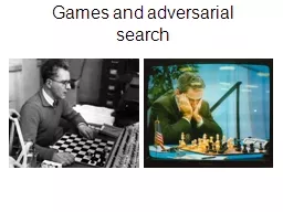
/
Games Outline I. Game as adversarial search Games Outline I. Game as adversarial search

Games Outline I. Game as adversarial search - PowerPoint Presentation

stella
stella . @stella
Follow
65 views
Uploaded On 2023-11-03

Games Outline I. Game as adversarial search - PPT Presentation

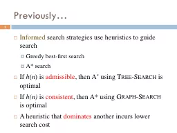
II The minimax algorithm Figuresimages are from the textbook site or by the instructor Otherwise the source is specifically cited unless citation would make little sense due to the triviality of generating such an image ID: 1028054

state game max min game state min max player move minimax chess players node games tree optimal utility search

Share:

Link:

Embed:

Download Presentation from below link

Download Presentation The PPT/PDF document "Games Outline I. Game as adversarial sea..." is the property of its rightful owner. Permission is granted to download and print the materials on this web site for personal, non-commercial use only, and to display it on your personal computer provided you do not modify the materials and that you retain all copyright notices contained in the materials. By downloading content from our website, you accept the terms of this agreement.


Presentation Transcript

1. GamesOutlineI. Game as adversarial searchII. The minimax algorithm* Figures/images are from the textbook site (or by the instructor) . Otherwise, the source is specifically cited unless citation would make little sense due to the triviality of generating such an image.III. Alpha-beta pruning

2. I. GamesCompetitive environments: goals are in conflict. Adversarial search problems (games)

3. Why Study Games?  Multiagent environment Aggregate of a large number of agents for predictions (e.g., price rise). Nondeterminism made by adversarial agents.  Introduction of new modeling techniques.  Mathematical game theory – an important branch of economics. Appealing subject for study in AI. Hard – engaging the intellectual faculties of humans.  Abstract nature – easy to represent with small number of actions.  Fun and entertaining. Each player has chosen a strategy and no player can increase own expected payoff by changing their strategy while the other players keep theirs unchanged,.Nash equilibrium for a non-cooperative game:Nobel Prize in Economics (1994)John Nash (Princeton)* Photo from https://www.nobelprize.org/prizes/economic-sciences/1994/nash/facts/ .

4. History of Computer Games 1950 Claude Shannon, Programming a Computer for Playing Chess.“Father of information theory”National Medal of Science (1966)Claude Shannon (MIT)* Photo from https://en.wikipedia.org/wiki/Claude_Shannon. 1956 John McCarthy conceives alpha-beta search. 1982 BELLE becomes the first chess program to achieve master status. 1997 Deep Blue (IBM) defeats world chess champion Garry Kasparov. 2017 AlphaGo (Alphabet) defeats world’s no. 1 Go player Ke Jie.  Visual pattern recognition Reinforcement learning Neural networks Monte Carlo tree search 2018 AlphaZero (Alphabet) defeats top programs in Go, chess, shogi. 2019 Pluribus (CMU) defeats top-ranked players in Texas hold’em games with six players. 1984 Judea Pearl, Heuristics.

5. Types of Games Games with deterministic, perfect information (e.g., chess, go, checkers) Stochastic games (e.g., backgammon) Partially observable games (e.g., bridge, poker)

6. II. Two-Player Game Perfect information – fully observable. Zero sum – what is good for one player is just as bad for the other.move action position state MAX and MIN: two players.

7. Formal Definition of a Game : initial state – game setup.  TO-MOVE: the player to move in the state.  ACTIONS: the set of legal moves in the state. At a state :   RESULT: the transition model defining the next state from taking action .   IS-TERMINAL: to test if the game is over, i.e., if is a terminal state.   UTILITY : a utility function to return a value to the player if the game ends in terminal state . e.g., in chess, win (1), loss (0), draw (1/2)Total payoff for all players is constant (zero-sum game):  

8. State Space Graph (Tic-Tac-Toe)Vertices states and edges moves  terminal nodes ( distinct states)  for chess! 

9. Two-Ply Game TreeUtility valuesPly: one move by a player

10. Optimal StrategyWork out the minimax value of every state in the tree, MINIMAX assuming both players play optimally:  MAX moves to a state of maximum value at its turn; MIN moves to a state of minimum value at its turn.MINIMAX  UTILITY MAX if IS-TERMINAL RESULT if TO-MOVE MAX RESULT if TO-MOVE MIN 

11. Minimax Value at Min NodesMIN: choose a move to a MAX node with the lowest value.Minimax values

12. Minimax Value at a Max NodeMAX: choose a move to a MIN node with the highest value.

13. Solution of the GameBest move for MAX:  Best move for MIN in response:  

14. The Minimax Search Algorithm

15. Algorithm ExecutionDepth-first search with backed-up value on return from a node.    

16. Summary on MinimaxTime:  Space:  max depthbranchingfactor Complete if the game tree is finite. Optimal against an optimal opponent. If MIN does not play optimally, 1) MAX will play at least as well as an optimal player; 2) but there may be a better strategy against the suboptimal MIN. Complexities: Chess: and for a reasonable game.Exact optimal solution infeasible!  

17. Multiplayer Games Every node now has a vector of values. Extend the minimax algorithm: for three players , ,  Backed-up value at a node utility vector of the successor state with the highest value for the player choosing at  Utility vector

18. III. Alpha-Beta Cutoff #states is exponential in the depth of the game tree. But we can often compute the correct minimax decision by pruning large parts of the tree that do not affect the outcome.

19. Re-examining the Game Tree  MIN node returns a value   Fig. 5.5 in the textbook incorrectly executes the algorithm in Fig. 5.7.possible range of the returned value]     

20. Cont’d  ) pruned ]   ]  (no change in value)  

21. Cont’d   MINIMAXroot maxminminmin maxmin max where = min               (no changein value) 

22. A Larger Example (Wikipedia)Current min value (4) current max value (5) at parent; no need for further exploration  Current min (5) at node current max (6) at parent