/
What to remember from exercises What to remember from exercises

What to remember from exercises - PowerPoint Presentation

tatiana-dople
tatiana-dople . @tatiana-dople
Follow
372 views
Uploaded On 2017-06-08

What to remember from exercises - PPT Presentation

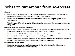
General Cluster results are sensitive to the parameter settings threshold to cut the tree for hierarchical clustering and number of clusters for K means Cluster results can be visualized by a ID: 557421

space clustering tmp rescaled clustering space rescaled tmp hierarchical correlation data clusters cluster original distance results golub means plotted

Share:

Link:

Embed:

Download Presentation from below link

Download Presentation The PPT/PDF document "What to remember from exercises" is the property of its rightful owner. Permission is granted to download and print the materials on this web site for personal, non-commercial use only, and to display it on your personal computer provided you do not modify the materials and that you retain all copyright notices contained in the materials. By downloading content from our website, you accept the terms of this agreement.


Presentation Transcript

Slide1

What to remember from exercises

General

Cluster

results are sensitive to the parameter settings (threshold to cut the tree for hierarchical clustering and number of clusters for K means

)

Cluster results can be visualized by a

heatmap

in either the ‘original space’ or the ‘rescaled space

With K means different runs give different results even when the same parameters are being

used

Rescaling data and effect on clustering

Cluster results with correlation distance on the original space and the rescaled space are exactly the same (also best visible with hierarchical clustering)

Cluster results with Euclidean distance in the rescaled space and correlation are exactly the same (a least when using hierarchical clustering p 9 and 20)

Cluster results with Euclidean distance on the original space and the rescaled space are different (also best visible with hierarchical clustering) (see slides)

Directionality of the matrix

Clustering

can be performed in the gene or in the patient

direction

(depends on whether the

datamatrix

was transposed)Slide2

P1 P2 P3 P4 … Pm

G1

G2

G3

G4

Gn

Patient profiles

Patients/conditions =observations

Genes = variables

P1 P2 P3 P4 … Pm

G1

G2

G3

G4

Gn

Gene profiles

Patients/conditions = variables

Genes = observationsSlide3

expressie

A’’

1

2

3

n

X=0

x

11

x

12

x

1n

x

13

x

14

expressie

A’’

1

2

3

n

X=0

x

11

x

12

x

1n

x

13

x

14

Mean centering

Variance rescaling

rescalingSlide4

A’

A’’

X2

X 1

A

A’

A’’

X2

X 1

A

Euclidean distance = 0

Pearson correlation = 1

Euclidean distance <> 0

Pearson correlation = 1Slide5

Effect of distance metrics/rescaling on cluster results

Cluster results with correlation distance on the original space and the rescaled space are exactly the same (also best visible with hierarchical clustering) p2

Cluster results with Euclidean distance in the rescaled space and correlation are exactly the same (a least when using hierarchical clustering p 9 and 20)

Cluster results with Euclidean distance on the original space and the rescaled space are different (also best visible with hierarchical clustering)

Why would this best be visible with the hierarchical clustering?Slide6

Hierarchical clustering using Euclidean distance on the rescaled data (100 clusters, query gene)

Hierarchical clustering using Euclidean distance on the original data

Plotted in the original space

Plotted in the original space

Plotted in the rescaled space

Plotted in the rescaled spaceSlide7

K-Means clustering using Euclidian distance on the original data (500 clusters, query gene)

K-means clustering using Euclidian distance on the rescaled data

Plotted in the original space

Plotted in the original space

Plotted in the rescaled space

Plotted in the rescaled space

This one could never be detected by clustering in the original spaceSlide8

kmeangolub100$cluster[1042]

tmp.data

<-

golub

breaks.tmp

<-

seq

(min(tmp.data

), max(

tmp.data), length=(40+1) )

heatmap.2(golub

[which(

kmeangolub100$cluster == kmeangolub100$cluster[1042] ),], col=

bluered(40), scale="none", density.info='none', trace="none", breaks=breaks.tmp

)

K-means (correlation)

What is this code doing. If you rerun K means, will the query gene end up in the same cluster? Why/ why not

Run1

Run2

If you look at the gene level: some genes reoccur together with the query genes

in the different clusters : stable signals!Slide9

c

u

c

v

Hierarchical clusteringSlide10

Hierarchical clustering

W

hat is the following code doing?, what happens if I choose k=100?

d.correlation <- as.dist(1 -

cor(t(golub)))hclust.correlation

<- hclust(d.correlation, method = ‘complete’)

clusters.correlation10 <- cutree(hclust.correlation, k=10)

table(clusters.correlation10)#1 2 3 4 5 6 7 8 9 10 #308 237 258 580 315 464 345 238 235 71

 #308 + 237+ 258 +580+ 315 +464+ 345+ 238+ 235 + 71 =3051Slide11

table(clusters.correlation100)

1 2 3 4 5 6 7 8 9 10 11 12 13 14 15 16 17 18 19 20

23 62 45 68 29 9 16 75 101 52 29 114 32 10 11 26 30 28 19 24

21 22 23 24 25 26 27 28 29 30 31 32 33 34 35 36 37 38 39 40

68 34 27 35 22 60 15 49 42 81 39 55 72 26 70 54 44 48 25 22

41 42 43 44 45 46 47 48 49 50 51 52 53 54 55 56 57 58 59 60

33 45 36 29 25 19 85 22 19 11 23 26 7 44 33 15 28 42 18 34

61 62 63 64 65 66 67 68 69 70 71 72 73 74 75 76 77 78 79 80

25 27 12 23 26 46 24 19 12 14 13 11 28 24 17 50 15 13 22 44

81 82 83 84 85 86 87 88 89 90 91 92 93 94 95 96 97 98 99 100

13 8 28 18 24 15 16 10 7 18 15 26 16 12 14 17 14 10 12 8

Hierarchical clusteringSlide12

heatmap.2(

golub_rescaled

[which(clusters.correlation100==1),], scale="none", cexRow=0.5, cexCol=0.8, col=

topo.colors(20), trace="none", Colv=FALSE, dendrogram = ‘row’)

Hierarchical clustering

Default plot in the rescaled spaceSlide13

Hierarchical clustering

#color scheme

fixed based on the global

rescaled dataset (-5 en 5 is de range)tmp.data <-golub_rescaled

breaks.tmp <- seq(min(tmp.data), max(tmp.data

), length=(40+1) )heatmap.2(golub_rescaled[which(clusters.correlation100==1),], col=

bluered(40), scale="none", density.info='none', trace="none", breaks=breaks.tmp)

Advantage of the rescaled plots:

Comparison between cluster results possible

Cluster to which biomarker belongs

Cluster 1Slide14
Slide15

kmeangolub10 =

kmeans

(d.correlation,10)

table(kmeangolub10$cluster

)

1 2 3 4 5 6 7 8 9 10

183 234 282 365 302 338 327 431 250 339

183 + 234 + 282 + 365 + 302 + 338+ 327+ 431 +250 +339 =3051 (dim(

golub

)

kmeangolub100

=

kmeans(d.correlation,100)

table(kmeangolub100$cluster) 1 2 3 4 5 6 7 8 9 10 11 12 13 14 15 16 17 18 19 20

38 28 40 25 36 42 37 27 36 30 17 21 25 25 24 34 33 38 23 28 21 22 23 24 25 26 27 28 29 30 31 32 33 34 35 36 37 38 39 40

24 39 30 24 61 31 27 25 28 30 25 29 43 21 28 17 49 48 24 29

41 42 43 44 45 46 47 48 49 50 51 52 53 54 55 56 57 58 59 60

32 35 28 23 29 21 18 25 34 36 26 27 24 32 33 30 29 41 57 46 61 62 63 64 65 66 67 68 69 70 71 72 73 74 75 76 77 78 79 80

K-means

Similar to hierarchical clustering K means assigns all genes to clusters/ the number of clusters you define determines the size of the clustersSlide16
Slide17

What to expected from exam

General questions:

What is guilt by

associationYes/ no questionsClustering with K Means and the correlation metric gives different results when applied to the original versus the rescaled data

ExercisesWhat is this code doingd.correlation <- as.dist(1 -

cor(t(golub)))hclust.correlation

<- hclust(d.correlation, method = ‘complete’)

clusters.correlation10 <- cutree(hclust.correlation, k=10)Slide18

PCASlide19

#

color scheme

fixed based on the global dataset (-1.6, 3.8)

tmp.data <-golubbreaks.tmp <-

seq(min(tmp.data), max(tmp.data), length=(40+1) )

heatmap.2(golub[which(clusters.correlation100==1),], col=

bluered(40), scale="none", density.info='none', trace="none", breaks=breaks.tmp,

Colv=FALSE, dendrogram = ‘row’)

Hierarchical clustering

#

color scheme fixed based on the global rescaled dataset (-1.6, 3.8)

tmp.data <-golub_rescaledbreaks.tmp <-

seq(min(tmp.data), max(tmp.data), length=(40+1) )heatmap.2(

golub_rescaled[which(clusters.correlation100==1),], col=bluered(40), scale="none", density.info='none', trace="none", breaks=breaks.tmp,

Colv=FALSE, dendrogram = ‘row’)

Given two codes and their results. What is the difference ?What can you observe from the different plotsSlide20

Hierarchical clustering

Hierarchical clustering/ correlation/500 clusters (p10)

golub.gnames

[which(clusters.correlation500 == clusters.correlation500[1042]),2]

[1] "KIAA0216 gene"

*[2] "

Calmodulin

Type I" [3] "Terminal transferase

mRNA" *[4] "CCND3 Cyclin D3"

[5] "TFIID subunit TAFII55 (TAFII55) mRNA" [6] "Hlark

mRNA" [7] "mRNA (clone C-2k) mRNA for serine/threonine protein kinase" [8] "NUCLEAR FACTOR RIP140"

* [9] "PROBABLE G PROTEIN-COUPLED RECEPTOR LCR1 HOMOLOG" [10] "Transcriptional activator hSNF2b"

Genes closest to the ‘query gene

’ in the absolute space and in the rescaled space (on which the clustering was based) -> rescaling will affect the clustering