Basic pulse sequences Gradient Echo GRE A class of pulse sequences that is primarily used for fast scanning 3D volume imaging Cardiac imaging Gradient reversal on the frequencyencoded axis forms the echo ID: 409327
Download Presentation The PPT/PDF document "G16.4427 Practical MRI 1" is the property of its rightful owner. Permission is granted to download and print the materials on this web site for personal, non-commercial use only, and to display it on your personal computer provided you do not modify the materials and that you retain all copyright notices contained in the materials. By downloading content from our website, you accept the terms of this agreement.
Slide1
G16.4427 Practical MRI 1
Basic pulse sequencesSlide2
Gradient Echo (GRE)
A class of pulse sequences that is primarily used for fast scanning
3D volume imaging
Cardiac imaging
Gradient reversal on the frequency-encoded axis forms the echo
A readout
prephasing
gradient lobe
dephases
the spins, then they are
rephased
with a readout gradient with opposite polarity
Can be fast because the flip angle is less than 90°
Why does that allows GRE to be fast?Slide3
Gradient Echo (GRE)
A class of pulse sequences that is primarily used for fast scanning
3D volume imaging
Cardiac imaging
Gradient reversal on the frequency-encoded axis forms the echo
A readout
prephasing
gradient lobe
dephases
the spins, then they are
rephased
with a readout gradient with opposite polarity
Can be fast because the flip angle is less than 90°
Fast T
1
recovery
short TR can be used (e.g. 2-50 ms)Slide4
Small Flip-Angle RF Pulse
What property of the small flip angle RF pulse is evident from this illustration?
Bernstein et al
. (2004) Handbook
of MRI
Pulse SequencesSlide5
Example of a GRE Pulse Sequence
The peak of the GRE occurs when the area under the two gradient lobes is equal.
Bernstein et al
. (2004) Handbook
of MRI
Pulse SequencesSlide6
T2 and T
2
*
Dephasing
T
2
dephasing
:
Inherent to tissue typeMolecular environment
Magnetic fields constantly changing in timeT2
* dephasingImperfect static magnetic fieldAir pockets (e.g. lungs) in bodyMetal parts in body (e.g. stents, clips)Magnetic fields that are constant in time
All of this PLUS T2 dephasingSlide7
Transverse Relaxation
T
2
* is always shorter than T
2
Bernstein et al
. (2004) Handbook
of MRI
Pulse SequencesSlide8
Response to a Series of RF Excitations
The excitation pulse is the only RF pulse in each TR (unless preparation pulses are used)
With a sufficient number of excitation pulses,
M
z
reaches a steady state
GRE sequences can be classified by the response of the transverse magnetization
M
xy
Spoiled: if ~0 just before each excitation
Steady-state free precession (SSFP): if reaches a nonzero steady stateSlide9
Spoiling
Spoiling can be accomplished in different ways
The simplest method is to use TR ~ 5T
2
Practical only with interleaved multi-slice acquisitions
End-of-sequence gradient spoiler
Not effective at spoiling the transverse steady state
Spatially non uniform because gradients produce spatially varying fields
RF spoiling
Phase-cycle the RF excitation pulses according to a predetermined schedule (i.e. flip the magnetization down in a different direction each time)Slide10
RF Spoiling
Stripe pattern artifact due to the spatially varying field produced by the gradients. (e.g. when the phase-encoding gradient is used as a spoiler, so no phase rewinding lobe is used)
(Bright stripes are unspoiled regions)
Bernstein et al
. (2004) Handbook
of MRI
Pulse SequencesSlide11
RF Spoiling
Stripe pattern artifact due to the spatially varying field produced by the gradients. (e.g. when the phase-encoding gradient is used as a spoiler, so no phase rewinding lobe is used)
RF spoiling:
phase of the B
1
field for the
j
th
RF pulse in the rotating frame:
(equivalent to the phase twist imparted by the phase-encoding gradient)
The recommended value for the starting phase increment is ϕ
0
= 117
°
During each TR the received MR signal must be shifted by the same phase, so
that
k
-space data are consistent
(Bright stripes are unspoiled regions)
Bernstein et al
. (2004) Handbook
of MRI
Pulse SequencesSlide12
Steady State Mz
for Spoiled GRE
If the longitudinal magnetization at point A is
M
zA
, after the excitation pulse
M
zB
=
M
zAcosθIn the TR between points B and C, T1 relaxation occurs, so:
When a steady state is reached MzA =
M
zC
Bernstein et al
. (2004) Handbook
of MRI
Pulse SequencesSlide13
The signal
S
spoil
is caused by the gradient
rephasing
the FID at an echo time TE, so it is given by:
Which is equal to:
Ernst Angle
Richard Ernst
August 14, 1933
1991
Nobel Prize in Chemistry
“Ernst angle”
The flip angle that maximize the signal is:Slide14
SSFP-FID (FISP) And SSFP-Echo
Standard GRE with greater signal than spoiled pulse sequences
Often at the cost of less contrast
SSFP-Echo less used
Conditions for SSFP:
phase coherent (RF pulses have the
same phase, or sign alternation, in
the rotating frame)
TR < T
2
Accumulated phase is the same in
each TR (
same gradient area)
If met, than steady states for both
M
z
and
M
xy
will be established
(A FID-like signal just after the RF and a
time-reversed just before each pulse)
Bernstein et al
. (2004) Handbook
of MRI
Pulse SequencesSlide15
SSFP-FID (FISP) And SSFP-Echo
Chavhan
GB et
al
. (2008)
Radiographics
vol. 28(4)
Phase-coherent RF pulses with same flip-angle and constant TR < T
2
steady state
Post-excitation signal (S+), FID arising from most recent RF pulse
Echo reformation signal (S-) when residual echo is refocused at the time of the subsequent RF pulseSlide16
SSFP-FID And SSFP-Echo Signals
If TR >> T
2
Slide17
SSFP-FID And SSFP-Echo Signals
If TR >> T
2
If
θ
<< 1
(PD-weighting at low flip angles)Slide18
Balanced SSFP (True FISP)
For SSFP the gradient area on any axis must not vary among TR intervals
For Balanced SSFP the gradient area on any axis is zero during each TR
Peaks of SSFP-FID and SSFP-Echo combine at TE (coherent sum of two signals
The magnitude of the signal changes for sign alternated pulses
If the balanced SSFP signal is
rephased
in the center of the TR interval (i.e. TE = TR/2), the decay is governed by T
2
rather than T
2
*
decreasing TE can increase susceptibility weighting in balanced SSFP
(the contrary happens for spoiled GRE and SSFP-FID)
Used in practice because of greater signalSlide19
Balanced SSFP
Scheffler
K and
Lehnhardt
S (2003)
Eur
Radiol
vol. 13 Slide20
Artifacts of Balanced SSFP
In regions where a phase shift removes the sign alternation there is a signal loss
Banding artifact
Unwanted phase shifts are always present
Short TR (e.g. less than 7 ms) are needed
Question: are balanced SSFP easier or more difficult to implement at higher field strength?Slide21
Banding Artifacts in Balanced SSFP
Scheffler
K and
Lehnhardt
S (2003)
Eur
Radiol
vol. 13 Slide22
Examples of Banding ArtifactsSlide23
Artifacts of Balanced SSFP
In regions where a phase shift removes the sign alternation there is a signal loss
Banding artifact
Question:
for example what could cause a phase shift?
Unwanted phase shifts are always present
Short TR (e.g. less than 7 ms) are needed
Question: are balanced SSFP easier or more difficult to implement at higher field strength?Slide24
Artifacts of Balanced SSFP
In regions where a phase shift removes the sign alternation there is a signal loss
Banding artifact
Unwanted phase shifts are always present
Short TR (e.g. less than 7 ms) are needed
Question:
are balanced SSFP easier or more difficult to implement at higher field strength?Slide25
Artifacts of Balanced SSFP
In regions where a phase shift removes the sign alternation there is a signal loss
Banding artifact
Unwanted phase shifts are always present
Short TR (e.g. less than 7 ms) are needed
More difficult to implement at high field
Increased susceptibility variations
SAR associated with very short TRSlide26
Particular Cases of Balanced SSFP
For short TR (TR << T
2
< T
1
) the signal formula becomes:
Question:
what does the formula tells you about the signal from fluids in balanced SSFP images?Slide27
Particular Cases of Balanced SSFP
For short TR (TR << T
2
< T
1
) the signal formula becomes:
The signal is maximized for:
At flip angles ~ 90° becomes more highly T
2
/ T
1
weighted:
Max of nearly M
0
/2 when T
2
= T
1
extremely strong signal for a short TR pulse sequenceSlide28
Example
SSFP-FID and Spoiled GRE:
TR = 14 ms
TE = 6 ms
Balanced SSFP:
TR = 6 ms
TE = 3 msSlide29
Inversion Recovery (IR)
Pulse sequences with an inversion pulse followed by a time delay prior to an RF excitation
Produce images with T
1
-weighted contrast.
Why?Slide30
Inversion Recovery (IR)
Pulse sequences with an inversion pulse followed by a time delay prior to an RF excitation
Produce images with T
1
-weighted contrast.
Time delay is know as the inversion time (TI)
Consists of two parts:
Inversion pulse, spoiler gradient (optional), slice selection gradient (if selective inversion pulse)
A self-contained pulse sequence (e.g. GRE) after TI
Require long TR (2-11
s
) to preserve the contrast2D IR sequences more frequently usedBenefits from real rather than magnitude reconstructionWhy?Slide31
Inversion Recovery (IR)
Pulse sequences with an inversion pulse followed by a time delay prior to an RF excitation
Produce images with T
1
-weighted contrast.
Why?
Time delay is know as the inversion time (TI)
Consists of two parts:
Inversion pulse, spoiler gradient (optional), slice selection gradient (if selective inversion pulse)
A self-contained pulse sequence (e.g. GRE) after TI
Require long TR (2-11
s) to preserve the contrast2D IR sequences more frequently usedBenefits from real rather than magnitude reconstructionMz
ranges from –M0 and +M0
increased tissue contrastSlide32
Diagram of IR Pulse Sequence
Besides T1-weighted images, what is another application of IR pulse sequences that we mentioned during a previous lecture?
Bernstein et al
. (2004) Handbook
of MRI
Pulse SequencesSlide33
Principles of IR
Immediately after the inversion pulse:
During the time interval TI
(for long TR)
If
θ
inv
= 180°:
If
θ
inv
= 90°:
Saturation Recovery
(SR)Slide34
IR and SR Curves
The TI value that nulls the longitudinal magnetization is called the “
nulling
time” or “zero-crossing point”
SR
IR
nulling
time
Bernstein et al
. (2004) Handbook
of MRI
Pulse SequencesSlide35
Examples of IR Applications
T
1
mapping
A series of IR images are acquired from the same location with different TI (everything else the same)
Long TR used to avoid signal saturation
Non-linear fitting (for magnitude IR, first need to obtain the zero-crossing and negate signals before it)
Lipid suppression (STIR)
Improves contrast for lesions embedded in fat (e.g. edema in bone marrow), as lipids appear bright like many lesions in post-contrast
Water signal loss (any tissue with T
1
similar to fat)Long acquisition timeSlide36
Radiofrequency Spin Echo (SE)
Formed by an excitation pulse and one or more refocusing pulse
Usually a
90° pulse followed by 180° pulse
Typically 2D mode using interleaved
multislice
Allows to obtain a specific contrast weighting
Greater immunity to off-resonance artifacts
Why?Slide37
Radiofrequency Spin Echo (SE)
Formed by an excitation pulse and one (or more in multi-echo SE) refocusing pulse
Usually a
90° pulse followed by 180° pulse
Typically 2D mode using interleaved
multislice
Allows to obtain a specific contrast weighting
Greater immunity to off-resonance artifacts because of the 180
°
refocusing pulse
As T
2 > T2* heavily T
2-weighted images possible with long TE without much signal loss (dephasing)Only a single phase-encoding step in any TR intervalSlide38
Single-Echo SE
Bernstein et al
. (2004) Handbook
of MRI
Pulse SequencesSlide39
Determination of TE
The gradient area on the frequency-encoding axis determines the temporal location of the peak of the echo (when the area under readout gradient balances the area of the
prephasing
gradient lobe)
Sometimes
Δ
is nonzero due to systems imperfections (e.g. eddy currents that shift gradient lobes)
What is the effect?
Bernstein et al
. (2004) Handbook
of MRI
Pulse SequencesSlide40
Determination of TE
The gradient area on the frequency-encoding axis determines the temporal location of the peak of the echo (when the area under readout gradient balances the area of the
prephasing
gradient lobe)
Sometimes
Δ
is nonzero due to systems imperfections (e.g. eddy currents that shift gradient lobes)
The signal will have some T
2
* weighting
Note: some specialized sequences use
nonzero
Δ
intentionally
Bernstein et al
. (2004) Handbook
of MRI
Pulse SequencesSlide41
Partial-Echo SE
What differences do you notice?
Bernstein et al
. (2004) Handbook
of MRI
Pulse SequencesSlide42
Partial-Echo SE
The peak of the echo (not the center of the readout) occurs when the RF spin would have refocused in the absence of imaging gradients
Used to avoid T
2
* weighting of the signal and reduce minimum TE
Achieved by reducing the area of the
prephasing
lobe
Image reconstruction with partial Fourier methods
Bernstein et al
. (2004) Handbook
of MRI
Pulse SequencesSlide43
Signal Formula for SE
M
xy
negligible
(TR >> T2, or
spoiler gradient)
= 90°
= 180°
M
zA
short pulse (no T
1
relaxation
between A and B, or C and D)
Bernstein et al
. (2004) Handbook
of MRI
Pulse SequencesSlide44
Multi-Echo SE
The transverse magnetization can be repeatedly refocused into subsequent
SEs
by playing additional RF refocusing pulse
The series of echoes is called an echo train
Each echo number fits its own independent
k
-space
The length of the echo train is limited by T
2
decayIn most cases we are interested in 2 echoes (an early and a late one).
Question: if TR is long, what contrast will have the 2 resulting images?Slide45
Multi-Echo SE
The transverse magnetization can be repeatedly refocused into subsequent
SEs
by playing additional RF refocusing pulse
The series of echoes is called an echo train
Each echo number fits its own independent
k
-space
The length of the echo train is limited by T
2
decayIn most cases we are interested in 2 echoes (an early and a late one).
if TR is long, the two images will be PD- and T2-weighted, respectivelySlide46
Example of Dual-Echo SE Acquisition
Proton density-weighted
TE/TR = 17/2200 ms
T
2
-weighted
TE/TR = 80/2200 msSlide47
Dual-Echo SE
Bernstein et al
. (2004) Handbook
of MRI
Pulse SequencesSlide48
T2-Mapping
It is a common application of acquiring longer echo trains (otherwise more than two echoes per TR are rarely acquired in MRI)
In theory we can acquire long echo train of
SEs
and fit the signal intensity at each pixel to calculate T
2
In practice there are systematic errors that make it difficult to fit a
monoexponential
decay curve
Variable flip angle across slice profile
Stimulated echoes can introduce unwanted T
1-weighting variations into the echo-train signalsIf magnitude reconstruction is used, the noise floor has nonzero mean leading to incorrectly larger T2 valuesSlide49
Any questions?Slide50
See you on Thursday!