/
1 Statistics for  Business and Economics (13e) 1 Statistics for  Business and Economics (13e)

1 Statistics for Business and Economics (13e) - PowerPoint Presentation

tawny-fly
tawny-fly . @tawny-fly
Follow
351 views
Uploaded On 2018-11-18

1 Statistics for Business and Economics (13e) - PPT Presentation

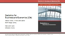
Anderson Sweeney Williams Camm Cochran 2017 Cengage Learning Slides by John Loucks St Edwards University Chapter 14 Part B Simple Linear Regression Using the Estimated Regression ID: 730395

regression residual standardized interval residual regression interval standardized plot cars estimate prediction analysis observation residuals output ads standard confidence

Share:

Link:

Embed:

Download Presentation from below link

Download Presentation The PPT/PDF document "1 Statistics for Business and Economics..." is the property of its rightful owner. Permission is granted to download and print the materials on this web site for personal, non-commercial use only, and to display it on your personal computer provided you do not modify the materials and that you retain all copyright notices contained in the materials. By downloading content from our website, you accept the terms of this agreement.


Presentation Transcript

Slide1

1

Statistics for

Business and Economics (13e)

Anderson, Sweeney, Williams, Camm, Cochran© 2017 Cengage Learning

Slides by John

Loucks

St. Edwards UniversitySlide2

Chapter

14, Part BSimple Linear Regression

Using the Estimated Regression Equation for

Estimation and PredictionResidual Analysis: Validating Model AssumptionsResidual Analysis: Outliers and Influential ObservationsComputer Solution2Slide3

Using the Estimated Regression Equation

for Estimation and Prediction

The margin of error is larger for a prediction interval.

A prediction interval is used whenever we want to predict an individual value of y for a new observation corresponding to a given value of x.

A

confidence interval

is an interval estimate of the

mean value of y

for a given value of

x

.

3Slide4

where:

confidence coefficient is 1 -

and t/2 is based on a t distribution with n - 2 degrees of freedomConfidence Interval Estimate of E(y

*

)

Prediction Interval Estimate of

y

*


4

Using the Estimated Regression Equation

for Estimation and PredictionSlide5

If 3 TV ads are run prior to a sale, we

expect

the mean number of cars sold to be:

Point Estimation 5Slide6

Estimate of the Standard Deviation of


Confidence Interval for

E(y*)


6Slide7

The 95% confidence interval estimate of the mean number of cars sold when 3 TV ads are run is:

25

+

4.6125 + 3.1824(1.4491)20.39 to 29.61 cars


7

Confidence Interval for

E

(

y

*

)Slide8

Estimate of the Standard

Deviation of

an Individual Value of

y*Prediction Interval for y*


s

pred

= 2.16025(1.20416) = 2.6013

8Slide9

The 95% prediction interval estimate of the number of cars sold in one particular week when 3 TV

ads

are run is:Prediction Interval for y*25 + 8.2825 + 3.1824(2.6013)

16.72 to 33.28 cars


9Slide10

Computer

Solution

The Regression tool can be used to perform a complete regression analysis.Excel also has a comprehensive tool in its Data Analysis package called

Regression

.

Up

to this point, you have seen how Excel can

be used

for various parts of a regression analysis.

10Slide11

11

Recall that the independent variable was named Ads and the dependent variable was named Cars in the example.

On the next slide we show Minitab output for the Reed Auto Sales example.

Performing the regression analysis computations without the help of a computer can be quite time consuming.Computer SolutionSlide12

12

The regression equation is

Cars = 10.0 + 5.00 Ads

Predictor

Coef

SE Coef

T

p

Constant

10.000

2.366

4.23

0.024

Ads

5.0000

1.080

4.63

0.019

S = 2.16025

R-sq = 87.7%

R-sq(adj) = 83.6%

Analysis of Variance

SOURCE

DF

SS

MS

F

p

Regression

1

100

100

21.43

0.019

Residual Err.

3

14

4.667

Total

4

114

Predicted Values for New Observations

New

Obs

Fit

SE Fit

95% C.I.

95% P.I.

1

25

1.45

(20.39, 29.61)

(16.72, 33.28)

Estimated

Regression

Equation

ANOVA

Table

Interval

Estimates

Minitab

OutputSlide13

13

Minitab prints the standard error of the estimate,

s, as well as information about the goodness of fit. .For each of the coefficients

b0 and b1, the output shows its value, standard deviation, t value, and p-value.Minitab prints the estimated regression equation as Cars = 10.0 + 5.00 Ads.The standard ANOVA table is printed.Also provided are the 95% confidence interval estimate of the expected number of cars sold and the 95% prediction interval estimate of the number of cars sold for an individual weekend with 3 ads.

Minitab OutputSlide14

14

Excel

Output

(top portion)Using Excel’s Regression Tool

A

B

C

9

10

Regression Statistics

11

Multiple R

0.936585812

12

R Square

0.877192982

13

Adjusted R Square

0.83625731

14

Standard Error

2.160246899

15

Observations

5

16

Slide15

15

Excel

Output

(middle portion)Using Excel’s Regression Tool

A

B

C

D

E

F

16

17

ANOVA

18

df

SS

MS

F

Significance F

19

Regression

1

100

100

21.4286

0.018986231

20

Residual

3

14

4.66667

21

Total

4

114

22Slide16

Note: Columns F-I are not shown.

Excel

Output

(bottom-left portion)16

Using Excel’s Regression ToolSlide17

Note: Columns C-E are hidden.

Excel

Output

(bottom-right portion)17

Using Excel’s Regression ToolSlide18

Residual Analysis

Much

of the residual analysis is based on

an examination of graphical plots.Residual for observation i The residuals provide the best information about e .

If

the assumptions about the error term

e

appear questionable

, the hypothesis tests about

the significance

of the regression relationship and

the interval

estimation results may not be valid.


18Slide19

Residual Plot Against

x

If the assumption that the variance of e

is the same for all values of x is valid, and the assumed regression model is an adequate representation of the relationship between the variables, then the residual plot should give an overall impression of a horizontal band of points. 19Slide20

x

0

Good Pattern

Residual


20

Residual Plot Against

xSlide21

x

0

Residual

Nonconstant

Variance


21

Residual Plot Against

xSlide22

x

0

Residual

Model Form Not Adequate


22

Residual Plot Against

xSlide23

Residuals

Observation

Predicted Cars Sold

Residuals

1

15

-1

2

25

-1

3

20

-2

4

15

2

5

25

2

23

Residual Plot Against

xSlide24

24

Residual Plot Against

xSlide25

Standardized Residual for

Observation

iStandardized Residuals

where:


25Slide26

Standardized Residual Plot

The standardized residual plot can provide insight about the assumption that the error term

e has a normal distribution.

If this assumption is satisfied, the distribution of the standardized residuals should appear to come from a standard normal probability distribution.26Slide27

Predicted y

Residual

Standardized

Residual

1

15

-1

-0.5345

2

25

-1

-0.5345

3

20

-2

-1.0690

4

15

2

1.0690

5

25

2

1.0690

Observation

Standardized Residuals

27

Standardized Residual PlotSlide28

Standardized Residual Plot

28

Standardized Residual PlotSlide29

All of the standardized residuals are between –1.5

and

+1.5 indicating that there is no reason to question the assumption that e has a normal distribution.29

Standardized Residual PlotSlide30

Outliers and Influential Observations

Detecting Outliers

Minitab classifies an observation as an outlier if its standardized residual value is < -2 or > +2.

This standardized residual rule sometimes fails to identify an unusually large observation as being an outlier.This rule’s shortcoming can be circumvented by using studentized deleted residuals.The |i th studentized deleted residual| will be larger than the |i th standardized residual|.

An

outlier

is an observation that is unusual in comparison with the other data.

30Slide31

End of Chapter

14, Part B31