/
Excel Chapter 3 Excel Chapter 3

Excel Chapter 3 - PowerPoint Presentation

tawny-fly
tawny-fly . @tawny-fly
Follow
412 views
Uploaded On 2016-03-03

Excel Chapter 3 - PPT Presentation

WhatIf Analysis Charting and Working with Large Worksheets Objectives Rotate text in a cell Create a series of month names Copy paste insert and delete cells Format numbers using format symbols ID: 240650

cell click button office click cell office button microsoft 2007 techniques concepts introductory format chart box display color ribbon

Share:

Link:

Embed:

Download Presentation from below link

Download Presentation The PPT/PDF document "Excel Chapter 3" is the property of its rightful owner. Permission is granted to download and print the materials on this web site for personal, non-commercial use only, and to display it on your personal computer provided you do not modify the materials and that you retain all copyright notices contained in the materials. By downloading content from our website, you accept the terms of this agreement.


Presentation Transcript

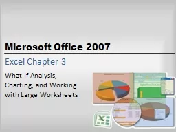
Slide1

Excel Chapter 3

What-If Analysis,

Charting, and Working

with Large WorksheetsSlide2

Objectives

Rotate text in a cell

Create a series of month names

Copy, paste, insert, and delete cellsFormat numbers using format symbolsFreeze and unfreeze titlesShow and format the system dateUse absolute cell references in a formula

2

Microsoft Office 2007: Introductory Concepts and TechniquesSlide3

Objectives

Use the IF function to perform a logical test

Use the Format Painter button to format cells

Create a 3-D Pie chart on a separate chart sheetColor and rearrange worksheet tabsChange the worksheet viewAnswer what-if questionsGoal seek to answer what-if questions

3

Microsoft Office 2007: Introductory Concepts and TechniquesSlide4

Plan Ahead

Plan the layout of the worksheet

Determine the necessary formulas and functions needed

Identify how to format various elements of the worksheetSpecify how the chart should convey necessary informationPerform what-if analysis and goal seeking using the best techniques

4

Microsoft Office 2007: Introductory Concepts and TechniquesSlide5

Starting Excel

Click the Start button on the Windows taskbar to display the Start menu

Point to All Programs on the Start menu and then point to Microsoft Office in the All Programs submenu

Click Microsoft Office Excel 2007 on the Microsoft Office submenuIf the Excel window is not maximized, click the Maximize button next to the Close button on its title bar to maximize the window

If the worksheet window in Excel is not maximized, click the Maximize button next to the Close button on its title bar to maximize the worksheet window within Excel

5

Microsoft Office 2007: Introductory Concepts and TechniquesSlide6

Entering the Worksheet Titles, Changing Workbook Properties, Applying a Theme, and Saving the Workbook

Click cell A1 and then enter Campus Clothiers as the worksheet title

Click cell A2 and then enter Semiannual Projected Gross Margin, Expenses, and Operating Income as the worksheet subtitle and then press the ENTER key

Click the Office Button, click Prepare on the Office Button menu, and then click Properties

Update the document properties with your name and any other relevant informationClick the Close button in the Document Properties pane

6

Microsoft Office 2007: Introductory Concepts and TechniquesSlide7

Entering the Worksheet Titles, Changing Workbook Properties, Applying a Theme, and Saving the Workbook

Apply the Trek theme to the worksheet by clicking the Themes button on the Page Layout tab on the Ribbon and then return to the Home tab on the Ribbon

With a USB flash drive connected to one of the computer’s USB ports, click the Save button on the Quick Access Toolbar

When Excel displays the Save As dialog box, type Campus Clothiers Semiannual Financial Projection in the File name text box

If necessary, click UDISK 2.0 (E:) in the Save in list (your USB flash drive may have a different name and letter). Click the Save button in the Save As dialog box to save the workbook

7

Microsoft Office 2007: Introductory Concepts and TechniquesSlide8

Rotating Text and Using the Fill Handle to Create a Series of Month Names

Select cell B3

Type January as the cell entry and then click the Enter box

Click the Format Cells: Alignment Dialog Box Launcher on the Ribbon to display the Format Cells dialog box

Click the 45° point in the Orientation area to move the Text hand in the Orientation area to the 45° point and to display 45 in the Degrees boxClick the OK button to rotate the text in cell B3 at a 45° angle and automatically increase the height of row 3 to best fit the rotated text

Point to the

fill

handle on the lower-right corner of cell B3

8

Microsoft Office 2007: Introductory Concepts and TechniquesSlide9

Rotating Text and Using the Fill Handle to Create a Series of Month Names

Drag the

fill

handle to the right to select the range C3:G3. Do not release the mouse buttonRelease the mouse button to create a month name series January through June in the range B3:G3 and copy the format in cell B3 to the range C3:G3

Click the Auto Fill Options button below the lower-right corner of the fill area to display the Auto Fill Options menuClick the Auto Fill Options button to hide the Auto Fill Options menu

Click cell H3, type

Total

, and then press the RIGHT ARROW key

9

Microsoft Office 2007: Introductory Concepts and TechniquesSlide10

Increasing Column Widths and Entering Rows Titles

Move the mouse pointer to the boundary between column heading A and column heading B so that the mouse pointer changes to a split double arrow

Drag the mouse pointer to the right until the ScreenTip displays, Width: 35.00 (322 pixels). Do not release the mouse button

Release the mouse button to change the width of column A

Click column heading B and then drag through column heading G to select columns B through G

10

Microsoft Office 2007: Introductory Concepts and TechniquesSlide11

Increasing Column Widths and Entering Rows Titles

Move the mouse pointer to the boundary between column headings B and C and then drag the mouse to the right until the ScreenTip displays, Width: 14.00 (133 pixels). Do not release the mouse button

Release the mouse button to change the width of columns B through G

Use the technique described in Step 1 to increase the width of column H to 15.00

Enter the row titles in the range A4:A18 as shown in two slides, but without the

indents

11

Microsoft Office 2007: Introductory Concepts and TechniquesSlide12

Increasing Column Widths and Entering Rows Titles

Click cell A5 and then click the Increase Indent button on the Ribbon

Select

the range A9:A13 and then click the Increase Indent button on the RibbonClick cell A19 to finish entering the row titles

12

Microsoft Office 2007: Introductory Concepts and TechniquesSlide13

Increasing Column Widths and Entering Rows Titles

13

Microsoft Office 2007: Introductory Concepts and TechniquesSlide14

Copying a Range of Cell to a Nonadjacent Destination Area

Select the range A9:A13 and then click the Copy button on the Home tab on the Ribbon to copy the values and formats of the range A9:A13 to the Office Clipboard

Click cell A19, the top cell in the destination area

Click the Paste button on the Ribbon to copy the values and formats of the last item placed on the Office Clipboard (range A9:A13) to the destination area A19:A23

Scroll down so row 5 appears at the top of the windowPress the ESC key to remove the marquee from the source area and disable the Paste button on the Ribbon

14

Microsoft Office 2007: Introductory Concepts and TechniquesSlide15

Copying a Range of Cell to a Nonadjacent Destination Area

15

Microsoft Office 2007: Introductory Concepts and TechniquesSlide16

Inserting a Row

Right-click row heading 21, the row below where you want to insert a row, to display the shortcut menu and the Mini toolbar

Click Insert on the shortcut menu to insert a new row in the worksheet by shifting the selected row 21 and all rows below it down one row

Click cell A21 in the new row and then enter Margin as the row title

Right-click row heading 24 and then click Insert on the shortcut menu to insert a new row in the worksheetClick cell A24 in the new row and then enter Revenue for Bonus as the row title

16

Microsoft Office 2007: Introductory Concepts and TechniquesSlide17

Inserting a Row

17

Microsoft Office 2007: Introductory Concepts and TechniquesSlide18

Entering Numbers with Format Symbols

Enter

100,000.00

in cell B19, 3.25% in cell B20,61.00% in cell B21, 9.00% in cell B22,

5.75% in cell B23, 4,750,000.00 in cell B24, and 17.00% in cell B25 to display the entries using a format based on the format symbols entered with the numbers

18

Microsoft Office 2007: Introductory Concepts and TechniquesSlide19

Entering Numbers with Format Symbols

19

Microsoft Office 2007: Introductory Concepts and TechniquesSlide20

Freezing Column and Row Titles

Press CTRL+HOME to select cell A1 and ensure that Excel displays row 1 and column A on the screen

Select cell

B4Click the View tab on the Ribbon and then click the Freeze Panes button on the Ribbon to display the Freeze Panes galleryClick Freeze Panes in the Freeze Panes gallery to freeze column A and rows 1 through 3

20

Microsoft Office 2007: Introductory Concepts and TechniquesSlide21

Freezing Column and Row Titles

21

Microsoft Office 2007: Introductory Concepts and TechniquesSlide22

Entering the Projected Monthly Sales

If necessary, click the Home tab on the Ribbon.

Enter

3383909.82 in cell B4, 6880576.15 in cell C4, 9742702.37

in cell D4, 4818493.53 in cell E4,

4566722.63

in cell F4, and

8527504.39

in cell

G4

Click cell H4 and then click the Sum button on the Ribbon twice to total the semiannual sales in cell H4

22

Microsoft Office 2007: Introductory Concepts and TechniquesSlide23

Entering the Projected Monthly Sales

23

Microsoft Office 2007: Introductory Concepts and TechniquesSlide24

Entering and Formatting the System Date

Click cell H2 and then click the Insert Function box in the formula bar

When Excel displays the Insert Function dialog box, click the Or select a category box arrow, and then select Date & Time in the list

Scroll down in the Select a function list and then click NOWClick the OK button

24

Microsoft Office 2007: Introductory Concepts and TechniquesSlide25

Entering and Formatting the System Date

When Excel displays the Function Arguments dialog box, click the OK button to display the system date and time in cell H2, using the default date and time format mm/

dd

/yyyy hh:mm.

Right-click cell H2 to display the shortcut menuClick Format Cells on the shortcut menu

When Excel displays the Format Cells dialog box, if necessary, click the Number tab

Click Date in the Category list. Scroll down in the Type list and then click 3/14/2001 to display a sample of the data in the active cell (H2) using the selected format in the Sample area

Click the OK button in the Format Cells dialog box to display the system date in the form mm/

dd

/

yyyy

25

Microsoft Office 2007: Introductory Concepts and TechniquesSlide26

Entering and Formatting the System Date

26

Microsoft Office 2007: Introductory Concepts and TechniquesSlide27

Entering a Formula Containing Absolute Cell References

Press CTRL+HOME and then click cell B5

Type

= (equal sign), click cell B4, type *(1-b21 and then press F4 to change b21 from a relative cell reference to an absolute cell reference

Type ) to complete the formulaClick the Enter box in the formula bar to display the result, 1319724.83, in cell B5, instead of the formula

Click cell B6, type = (equal sign), click cell B4, type — and then click cell B5

Click the Enter box in the formula bar to display the gross margin for January, 2064184.99, in cell B6

27

Microsoft Office 2007: Introductory Concepts and TechniquesSlide28

Entering a Formula Containing Absolute Cell References

28

Microsoft Office 2007: Introductory Concepts and TechniquesSlide29

Entering an IF Function

Click cell B9. Type =if(b4>=$b$24, $b$19,0) in the cell

Click the Enter box in the formula bar to display 0 in cell B9 (Figure 3–29),because the value in cell B4 (3383909.82) is less than the value in cell B24 (4,750,000)

29

Microsoft Office 2007: Introductory Concepts and TechniquesSlide30

Entering an IF Function

30

Microsoft Office 2007: Introductory Concepts and TechniquesSlide31

Entering the Remaining January Formulas

Click cell B10. Type

=b4*$b$20

and then press the DOWN ARROW key. Type =b4*$b$22 and then press the DOWN ARROW key. Type

=b4*$b$23 and then press the DOWN ARROW key. Type

=b4*$b$25

and then press the DOWN ARROW key

With cell B14 selected, click the Sum button on the Home tab on the Ribbon twice. Click cell B16. Type

=b6-b14

and then press the ENTER key

Press CTRL+ACCENT MARK (`) to instruct Excel to display the formulas version of the worksheet

When you are

finished

viewing the formulas version, press CTRL+ACCENT MARK (`) to instruct Excel to display the values version of the worksheet

31

Microsoft Office 2007: Introductory Concepts and TechniquesSlide32

Entering the Remaining January Formulas

32

Microsoft Office 2007: Introductory Concepts and TechniquesSlide33

Copying Formulas with Absolute Cell References Using the Fill Handle

Select the range B5:B16 and then point to the fill handle in the lower-right corner of cell B16

Drag the fill handle to the right to select the destination area C5:G16 to copy the formulas from the source area (B5:B16) to the destination area (C5:G16) and display the calculated amounts and Auto Fill Options button

33

Microsoft Office 2007: Introductory Concepts and TechniquesSlide34

Copying Formulas with Absolute Cell References Using the Fill Handle

34

Microsoft Office 2007: Introductory Concepts and TechniquesSlide35

Determining Row Totals in Nonadjacent Cells

Select the range H5:H6. Hold down the CTRL key and select the range H9:H14 and cell H16

Click the Sum button on the Ribbon to display the row totals in column H

35

Microsoft Office 2007: Introductory Concepts and TechniquesSlide36

Determining Row Totals in Nonadjacent Cells

36

Microsoft Office 2007: Introductory Concepts and TechniquesSlide37

Unfreezing the Worksheet Titles and Saving the Workbook

Press CTRL+HOME to select cell B4 and view the upper-left corner of the screen

Click the View tab on the Ribbon and then click the Freeze Panes button on the Ribbon to display the Freeze Panes gallery

Click Unfreeze Panes in the Freeze Panes gallery to unfreeze the titlesClick the Home tab on the Ribbon and then click the Save button on the Quick Access Toolbar

37

Microsoft Office 2007: Introductory Concepts and TechniquesSlide38

Unfreezing the Worksheet Titles and Saving the Workbook

38

Microsoft Office 2007: Introductory Concepts and TechniquesSlide39

Assigning Formats to Nonadjacent Ranges

Select the range B4:H4

While holding down the CTRL key, select the nonadjacent ranges B6:H6,B9:H9, B14:H14, and B16:H16, and then release the CTRL

keyClick the Format Cells: Number Dialog Box Launcher on the Ribbon to display the Format Cells dialog box

Click Currency in the Category list, select 2 in the Decimal places box, click $ in the Symbol list to ensure a dollar sign shows, and click the black font color ($1,234.10) in the Negative numbers list

Click the OK button

Select the range B5:H5

While holding down the CTRL key, select the range B10:H13, and then release the CTRL key

39

Microsoft Office 2007: Introductory Concepts and TechniquesSlide40

Assigning Formats to Nonadjacent Ranges

Click the Format Cells: Number Dialog Box Launcher on the Ribbon to display the Format Cells dialog

box

When Excel displays the Format Cells dialog box, click Currency in the Category list, select 2 in the Decimal places box, click None in the Symbol list so a dollar sign does not show, and click the black font color (1,234.10) in the Negative numbers list

Click the OK buttonPress CTRL+HOME to select cell A1 to display the formatted numbers

40

Microsoft Office 2007: Introductory Concepts and TechniquesSlide41

Assigning Formats to Nonadjacent Ranges

41

Microsoft Office 2007: Introductory Concepts and TechniquesSlide42

Formatting the Worksheet Titles

Click the column A heading to select column A

Click the Bold button on the Ribbon to bold all of the data in column A

Click cell A1 to select it. Click the Font Size box arrow on the Ribbon, and then click 36 in the Font Size listClick cell A2, click the Font Size box arrow, and then click 18 in the Font Size list

42

Microsoft Office 2007: Introductory Concepts and TechniquesSlide43

Formatting the Worksheet Titles

Select the range A1:H2 and then click the Fill Color button arrow on the Ribbon

Click Orange, Accent 1 (column 5, row 1) on the Fill Color palette

Click the Font Color button arrow on the Ribbon and then select White, Background 1 (column 1, row 1) on the Font Color palette

43Microsoft Office 2007: Introductory Concepts and TechniquesSlide44

Formatting the Worksheet Titles

44

Microsoft Office 2007: Introductory Concepts and TechniquesSlide45

Assigning Cell Styles to Nonadjacent Rows and Colors to a Cell

Select the range A3:H3 and apply the Heading 3 cell style

Select the range A6:H6 and while holding down the CTRL key, select the ranges A14:H14 and

A16:H16Apply the Total cell style

Click cell A4, click the Fill Color button arrow on the Ribbon, and then click the Orange, Accent 1 color (column 5, row 1) on the Fill Color paletteClick the Font Color button arrow on the Ribbon, and then click the White, Background 1 color (column 1, row 1) on the Font Color palette

45

Microsoft Office 2007: Introductory Concepts and TechniquesSlide46

Assigning Cell Styles to Nonadjacent Rows and Colors to a Cell

46

Microsoft Office 2007: Introductory Concepts and TechniquesSlide47

Copying a Cell’s Format Using the Format Painter Button

Select cell A4

Click the Format Painter button on the Ribbon and then move the mouse pointer onto the worksheet to cause the mouse pointer to change to a block plus sign with a paintbrush

Click cell A6 to assign the format of cell A4 to cell A6With cell A6 selected, click the Format Painter button on the Ribbon and then click cell A14

With cell A14 selected, click the Format Painter button on the Ribbon and then click cell A16

47

Microsoft Office 2007: Introductory Concepts and TechniquesSlide48

Copying a Cell’s Format Using the Format Painter Button

Select the range B16:H16, click the Fill Color button on the Ribbon, and then click the Orange, Accent 1 color (column 5, row 1) on the Fill Color palette

Click the Font Color button on the Ribbon, and then click the Background 1 color (column 1, row 1) on the Font Color palette

48

Microsoft Office 2007: Introductory Concepts and TechniquesSlide49

Copying a Cell’s Format Using the Format Painter Button

49

Microsoft Office 2007: Introductory Concepts and TechniquesSlide50

Formatting the What-If Assumptions Table and Saving the Workbook

Scroll down to view rows 18 through 25 and then click cell A18

Click the Font Size box arrow on the Ribbon and then click 14 in the Font Size list. Click the Italic button and then click the Underline button on the Ribbon

Select the range A19:B25, click the Font Size button on the Ribbon, and then click 8 in the Font Size list

Click cell D25 to deselect the range A19:B25 and display the What-If AssumptionsClick the Save button on the Quick Access

Toolbar

50

Microsoft Office 2007: Introductory Concepts and TechniquesSlide51

Formatting the What-If Assumptions Table and Saving the Workbook

51

Microsoft Office 2007: Introductory Concepts and TechniquesSlide52

Drawing a 3-D Pie Chart on a Separate Chart Sheet

Select the range B3:G3

While holding down the CTRL key, select the range B16:G16

Click the Insert tab on the RibbonClick the Pie button on the Ribbon to display the Pie gallery

52Microsoft Office 2007: Introductory Concepts and TechniquesSlide53

Drawing a 3-D Pie Chart on a Separate Chart Sheet

When Excel draws the chart, click the Move Chart button on the Ribbon to display the Move Chart dialog box

Click the New sheet option button and then type

3-D Pie Chart in the New sheet name textboxClick the OK button to move the chart to a new chart sheet with the name 3-D Pie Chart

53

Microsoft Office 2007: Introductory Concepts and TechniquesSlide54

Drawing a 3-D Pie Chart on a Separate Chart Sheet

54

Microsoft Office 2007: Introductory Concepts and TechniquesSlide55

Inserting a Chart Title and Data Labels

Click anywhere in the chart area outside the chart

Click the Layout tab on the Ribbon and then click the Chart Title button

Click the Centered Overlay Title command in the Chart Title gallerySelect the text in the chart title and then type Semiannual Financial Projection as the new chart title

55

Microsoft Office 2007: Introductory Concepts and TechniquesSlide56

Inserting a Chart Title and Data Labels

Select the text in the new title and then click the Home tab on the Ribbon

Click the Underline button to assign an underline font style to the chart title

Click the Layout tab on the Ribbon and then click the Legend button to display the Legend galleryPoint to None in the Legend gallery

Click None to turn off the legend on the chartClick the Data Labels button on the Ribbon and then click Outside End in the Data Labels gallery to display data labels outside the chart at the end of each slice

56

Microsoft Office 2007: Introductory Concepts and TechniquesSlide57

Inserting a Chart Title and Data Labels

If necessary, right-click any data label to select all of the data labels on the chart and to display the shortcut menu

Click the Format Data Labels command on the shortcut menu to display the Format Data Labels dialog box

If necessary, click the Series Name, Value, and Show Leader Lines check boxes to deselect them and then click the Category Name and Percentage check boxes to select them

Click the Close button to close the Format Data Labels dialog box and display the chart

57

Microsoft Office 2007: Introductory Concepts and TechniquesSlide58

Inserting a Chart Title and Data Labels

58

Microsoft Office 2007: Introductory Concepts and TechniquesSlide59

Rotating the 3-D Pie Chart

Click the 3-D Rotation button on the Ribbon to display the Format Chart Area dialog box

Click the Increase X Rotation button in the Rotation area of the Format Chart Area dialog box until the X rotation is at 250°

Click the Close button in the Format Chart Area dialog box to display the rotated chart

59

Microsoft Office 2007: Introductory Concepts and TechniquesSlide60

Rotating the 3-D Pie Chart

60

Microsoft Office 2007: Introductory Concepts and TechniquesSlide61

Applying a 3-D Format to the Pie Chart

Right-click the chart to display the shortcut menu

Click the Format Data Series command on the shortcut menu to display the Format Data Series dialog box and then click the 3-D Format category on the left side of the dialog

boxClick the Top button in the Bevel area to display the Bevel gallery

Click the Circle bevel button (column 1, row 1) in the Bevel gallery to add a bevel to the chartType 50 pt in the top Width box in the Bevel area of the dialog box and then type 50 pt in the uppermost Height box in the Bevel area of the dialog box to increase the width and height of the bevel on the chart

Click the Material button in the Surface area of the Format Data Series dialog box and then point to the Soft Edge button

Click the Close button in the Format Data Series dialog

box

61

Microsoft Office 2007: Introductory Concepts and TechniquesSlide62

Applying a 3-D Format to the Pie Chart

62

Microsoft Office 2007: Introductory Concepts and TechniquesSlide63

Exploding the 3-D Pie Chart and Changing the Color of the Slice

Click the slice labeled June twice (do not double-click) to select only the June slice

Right-click the slice labeled June to display the shortcut menu and then point to Format Data Point

When Excel displays the Format Data Point dialog box, drag the Point Explosion slider to the right until the Point Explosion box reads 28%

Click the Fill category on the left side of the dialog box

Click the Solid fill option button and then click the Color button to display the color

palette

63

Microsoft Office 2007: Introductory Concepts and TechniquesSlide64

Exploding the 3-D Pie Chart and Changing the Color of the Slice

Point to the Orange color in the Standard Colors area

Click the Orange color on the color palette and then click the Close button on the Format Data Point dialog box to change the color of the slice labeled June to orange

64

Microsoft Office 2007: Introductory Concepts and TechniquesSlide65

Exploding the 3-D Pie Chart and Changing the Color of the Slice

65

Microsoft Office 2007: Introductory Concepts and TechniquesSlide66

Changing the Colors of the Remaining Slices

Click the slice labeled January twice (do not double-click) to select only the January slice

Right-click the slice labeled January to display the shortcut menu and then point to Format Data Point

Click the Fill category on the left side of the dialog box

Click the Solid fill option button and then click the Color button to display the color paletteClick the Green color on the color palette and then click the Close button in the Format Data Point dialog box to change the color of the slice labeled January to green

Repeat

the previous steps

for the remaining four slices. Assign the following colors in the Standard Colors area of the color palette to each slice: February – Yellow; March – Light Blue; April – Red; May – Blue

66

Microsoft Office 2007: Introductory Concepts and TechniquesSlide67

Changing the Colors of the Remaining Slices

67

Microsoft Office 2007: Introductory Concepts and TechniquesSlide68

Renaming and Reordering the Sheets and Color their Tabs

Right-click the tab labeled 3-D Pie Chart at the bottom of the screen to display the shortcut menu

Point to the Tab Color command to display the color palette

Click Brown, Accent 2 (column 6, row 1) in the Theme Colors area to change the color of the tab to brown

Double-click the tab labeled Sheet1 at the bottom of the screen.Type

Semiannual Financial Projection

as the new sheet name and then press the ENTER key

Right-click the tab and then click Tab Color on the shortcut

menu

68

Microsoft Office 2007: Introductory Concepts and TechniquesSlide69

Renaming and Reordering the Sheets and Color their Tabs

Point to the Orange, Accent 1 (column 5, row 1) color in the Theme Colors area of the palette

Click Orange, Accent 1 (column 5, row 1) in the Theme Colors area to change the color of the tab to orange

Drag the Semiannual Financial Projection tab to the left in front of the 3-D Pie Chart tab to rearrange the sequence of the sheets and then click cell E18

69

Microsoft Office 2007: Introductory Concepts and TechniquesSlide70

Renaming and Reordering the Sheets and Color their Tabs

70

Microsoft Office 2007: Introductory Concepts and TechniquesSlide71

Checking Spelling in Multiple Sheets

With the Semiannual Financial Projection sheet active, press CTRL+HOME to select cell A1

Hold down the CTRL key and then click the 3-D Pie Chart tab

Click the Review tab on the Ribbon and then click the Spelling button on the RibbonCorrect any errors and then click the OK button when the spell check is complete

Click the Save button on the Quick Access Toolbar

71

Microsoft Office 2007: Introductory Concepts and TechniquesSlide72

Previewing and Printing the Workbook

Ready the printer. If both sheets are not selected, hold down the CTRL key and then click the tab of the inactive sheet

Click the Page Layout tab on the Ribbon and then click the Page Setup Dialog Box Launcher. Click the Page tab and then click Landscape. Click Fit to in the Scaling area

Click the Print Preview button in the Page Setup dialog box. When the preview of the first of the selected sheets appears, click the Next Page button at the top of the Print Preview window to view the next sheet. Click the Previous Page button to redisplay the first sheet

Click the Print button at the top of the Print Preview window. When Excel displays the Print dialog box, click the OK button to print the worksheet and chart

Right-click the Semiannual Financial Projection tab. Click Ungroup Sheets on the shortcut menu to deselect the 3-D Pie Chart

tab

Click the Save button on the Quick Access Toolbar

72

Microsoft Office 2007: Introductory Concepts and TechniquesSlide73

Previewing and Printing the Workbook

73

Microsoft Office 2007: Introductory Concepts and TechniquesSlide74

Shrinking and Magnifying the Viewing of a Worksheet or Chart

If cell A1 is not active, press CTRL+HOME

Click the View tab on the Ribbon and then click the Zoom button on the Ribbon to display a list of Magnifications in the Zoom dialog box

Click 75% and then click the OK button to shrink the display of the worksheet to 75% of its normal displayClick the Zoom In button on the status bar until the worksheet displays at 100%

74

Microsoft Office 2007: Introductory Concepts and TechniquesSlide75

Shrinking and Magnifying the Viewing of a Worksheet or Chart

75

Microsoft Office 2007: Introductory Concepts and TechniquesSlide76

Splitting a Window into Panes

Select cell D7, the intersection of the four proposed panes

If necessary, click the View tab on the Ribbon and then point to the Split button on the Ribbon

Click the Split button to divide the window into four panesUse the scroll arrows to show the four corners of the worksheet at the same time

76

Microsoft Office 2007: Introductory Concepts and TechniquesSlide77

Splitting a Window into Panes

77

Microsoft Office 2007: Introductory Concepts and TechniquesSlide78

Removing the Panes from the Window

Position the mouse pointer at the intersection of the horizontal and vertical split bars

When the mouse pointer changes to a four-headed arrow, double-click to remove the four panes from the window

78

Microsoft Office 2007: Introductory Concepts and TechniquesSlide79

Analyzing Data in a Worksheet by Changing Values

Use the vertical scroll bar to move the window so cell A6 is in the upper-left corner of the screen

Drag the vertical split box from the lower-right corner of the screen to the left so that the vertical split bar is positioned

as shown on the following slide

Use the right scroll arrow to view the totals in column H in the right paneEnter 75000 in cell B19, 2.25 in cell B20, and 14.50 in cell B25 which causes the semiannual operating income in cell H16 to increase from $9,459,176.31 to $

10,886,373.12

79

Microsoft Office 2007: Introductory Concepts and TechniquesSlide80

Analyzing Data in a Worksheet by Changing Values

80

Microsoft Office 2007: Introductory Concepts and TechniquesSlide81

Goal Seeking

Close the workbook without saving changes and then reopen it

Drag the vertical split box so that the vertical split bar is positioned as shown

Show column H in the right paneClick cell H16, the cell that contains the semiannual operating income

Click the Data tab on the Ribbon and then click the What-If Analysis button on the Ribbon to display the What-If Analysis menu

81

Microsoft Office 2007: Introductory Concepts and TechniquesSlide82

Goal Seeking

Click Goal Seek to display the Goal Seek dialog box with the Set cell box set to the selected cell, H16

When Excel displays the Goal Seek dialog box, click the To value text box, type 10500000 and then click the By changing cell box

Scroll down so row 4 is at the top of the screen

Click cell B25 on the worksheet to assign cell B25 to the By changing cell boxClick the OK button to goal seek for the value $10,500,000.00 in cell H16

Click the Cancel button in the Goal Seek Status dialog

box

82

Microsoft Office 2007: Introductory Concepts and TechniquesSlide83

Goal Seeking

83

Microsoft Office 2007: Introductory Concepts and TechniquesSlide84

Quitting Excel

Click the Close button on the title bar

If the Microsoft Excel dialog box is displayed, click the No

button84

Microsoft Office 2007: Introductory Concepts and TechniquesSlide85

Summary

Rotate text in a cell

Create a series of month names

Copy, paste, insert, and delete cellsFormat numbers using format symbolsFreeze and unfreeze titlesShow and format the system dateUse absolute cell references in a formula

85

Microsoft Office 2007: Introductory Concepts and TechniquesSlide86

Summary

Use the IF function to perform a logical test

Use the Format Painter button to format cells

Create a 3-D Pie chart on a separate chart sheetColor and rearrange worksheet tabsChange the worksheet viewAnswer what-if questionsGoal seek to answer what-if questions

86

Microsoft Office 2007: Introductory Concepts and TechniquesSlide87

87

Homework #7

In the lab

#1Page EX

233-236Parts 1 and 2 only Slide88

Excel Chapter 3 Complete