1 Chapter 6 Queueing systems Learning objectives :

slide1. 1 Chapter 6
Queueing systems Learning objectives :
Little's law
Impact of the randomness on performances of queueing systems
Product-form solutions

Textbook :
C. Cassandras and S. Lafortune, Introduction to Discrete Event Systems, Springer
S.M. Ross, Stochastic Process, John Wiley & Sons<br>
slide2. 2 Plan Introduction
Classification of queueing systems
Little's law
Single stage queuing systems
Queuing networks
Non Markovian queueing systems<br>
slide3. 3 Introduction<br>
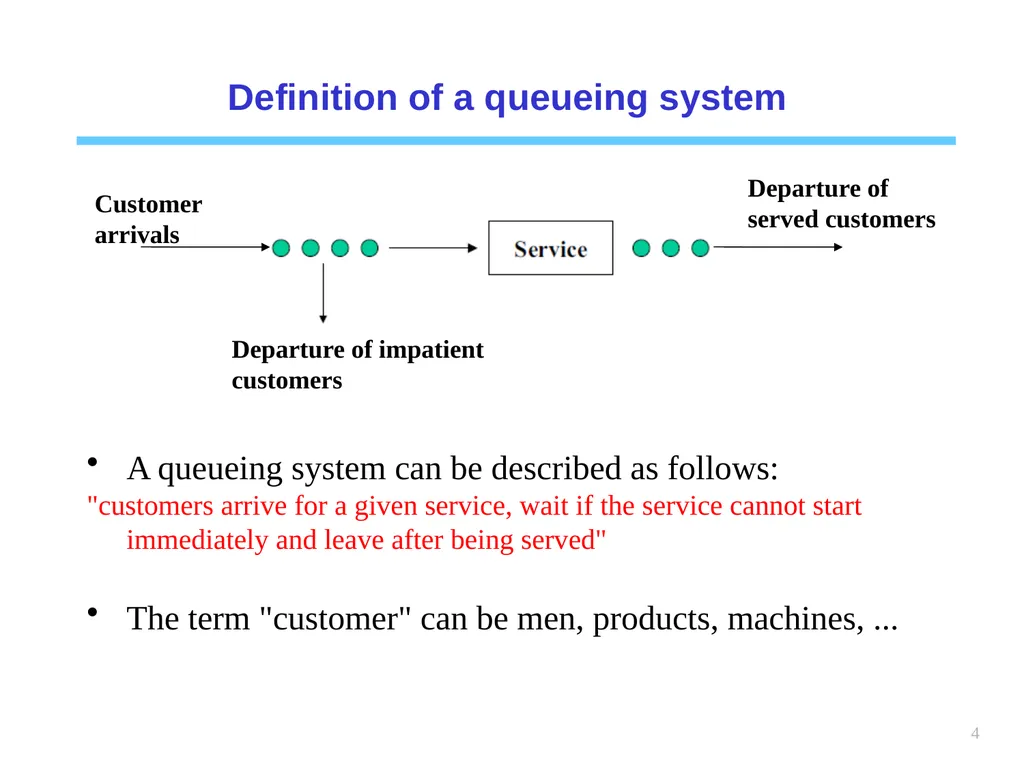
slide4. 4 Definition of a queueing system Customer arrivals Departure of impatient customers Departure of served customers A queueing system can be described as follows:
"customers arrive for a given service, wait if the service cannot start immediately and leave after being served"

The term "customer" can be men, products, machines, ...<br>
slide5. 5 History of queueing theory The theory of queueing systems was developed to provide models for forecasting behaviors of systems subject to random demand.
The first problems addressed concerned congestion of telephone traffic (Erlang, "the theory of probabilities and telephone conversations ", 1909)
Erlang observed that a telephone system can be modeled by Poisson customer arrivals and exponentially distributed service times
Molina, Pollaczek, Kolmogorov, Khintchine, Palm, Crommelin followed the track<br>
slide6. 6 Interests of queueing systems Queueing theory found numerous applications in:

– Trafic control (communication networks, air traffic, …)
– Planing (manufacturing systems, computer programmes, …)
– Facility dimensioning (factories, ...)<br>
slide7. 7 Classification of queueing systems<br>
slide8. 8 Characteristics of simple queueing systems Queueing systems can be characterized with several criteria:

Customer arrival processes
Service time
Service discipline
Service capacity
Number of service stages<br>
slide9. 9 Notation of Kendall The following is a standard notation system of queueing systems

T/X/C/K/P/Z with

– T: probability distribution of inter-arrival times
– X: probability distribution of service times
– C: Number of servers
– K: Queue capacity
– P: Size of the population
– Z: service discipline<br>
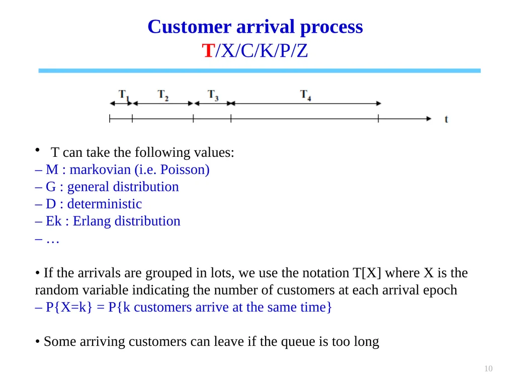
slide10. 10 Customer arrival process
T/X/C/K/P/Z T can take the following values:
– M : markovian (i.e. Poisson)
– G : general distribution
– D : deterministic
– Ek : Erlang distribution
– …

• If the arrivals are grouped in lots, we use the notation T[X] where X is the random variable indicating the number of customers at each arrival epoch
– P{X=k} = P{k customers arrive at the same time}

• Some arriving customers can leave if the queue is too long<br>
slide11. 11 Service times
T/X/C/K/P/Z X can take the following values:
– M : markovian (i.e. exponential)
– G : general distribution
– D : deterministic
– Ek : Erlang distribution
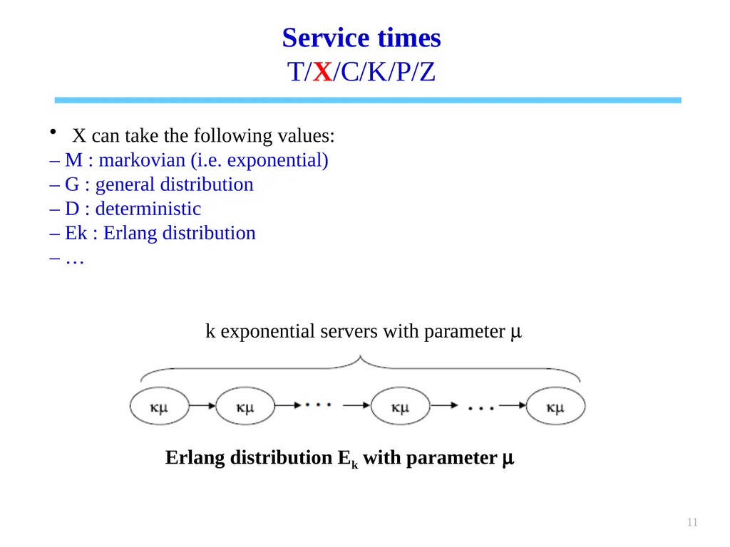
– … Erlang distribution Ek with parameter m k exponential servers with parameter m<br>
slide12. 12 Number of servers
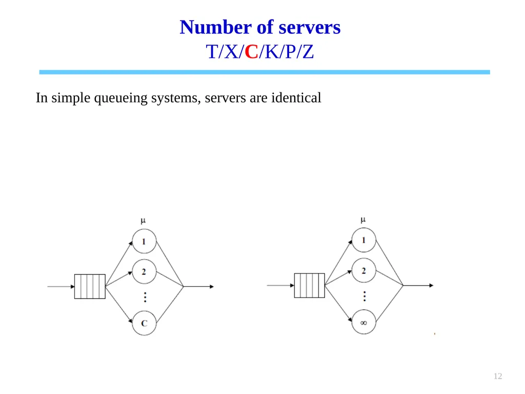
T/X/C/K/P/Z In simple queueing systems, servers are identical<br>
slide13. 13 Queue capacity
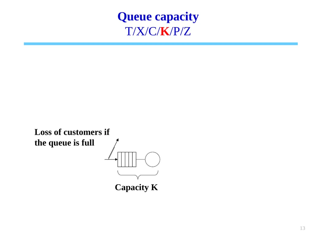
T/X/C/K/P/Z Loss of customers if the queue is full Capacity K<br>
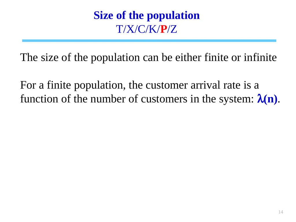
slide14. 14 Size of the population
T/X/C/K/P/Z The size of the population can be either finite or infinite

For a finite population, the customer arrival rate is a function of the number of customers in the system: l(n).<br>
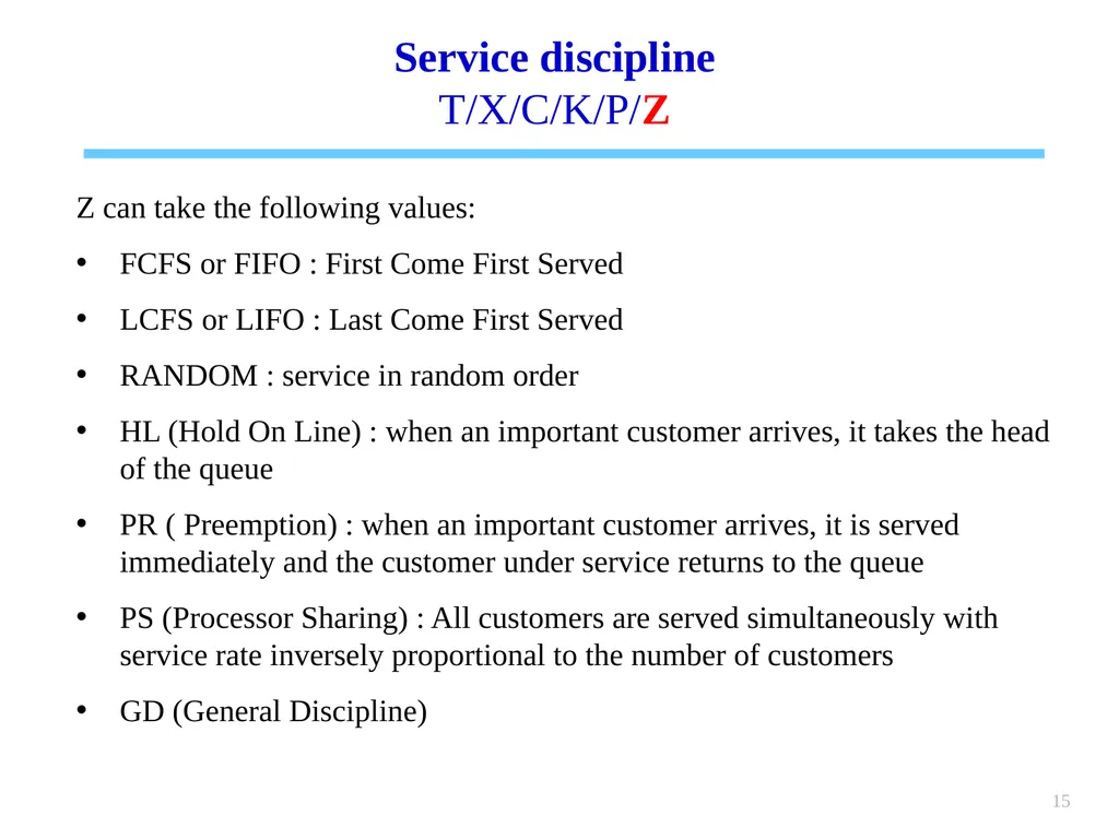
slide15. 15 Service discipline
T/X/C/K/P/Z Z can take the following values:
FCFS or FIFO : First Come First Served
LCFS or LIFO : Last Come First Served
RANDOM : service in random order
HL (Hold On Line) : when an important customer arrives, it takes the head of the queue
PR ( Preemption) : when an important customer arrives, it is served immediately and the customer under service returns to the queue
PS (Processor Sharing) : All customers are served simultaneously with service rate inversely proportional to the number of customers
GD (General Discipline)<br>
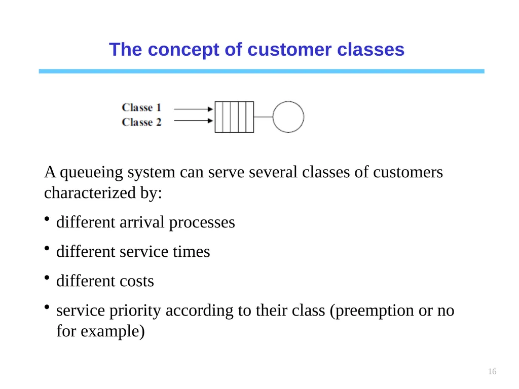
slide16. 16 The concept of customer classes A queueing system can serve several classes of customers characterized by:
different arrival processes
different service times
different costs
service priority according to their class (preemption or no for example)<br>
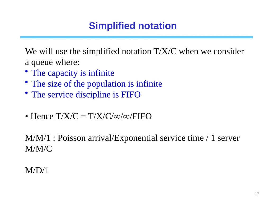
slide17. 17 Simplified notation We will use the simplified notation T/X/C when we consider a queue where:
The capacity is infinite
The size of the population is infinite
The service discipline is FIFO

• Hence T/X/C = T/X/C///FIFO

M/M/1 : Poisson arrival/Exponential service time / 1 server
M/M/C

M/D/1<br>
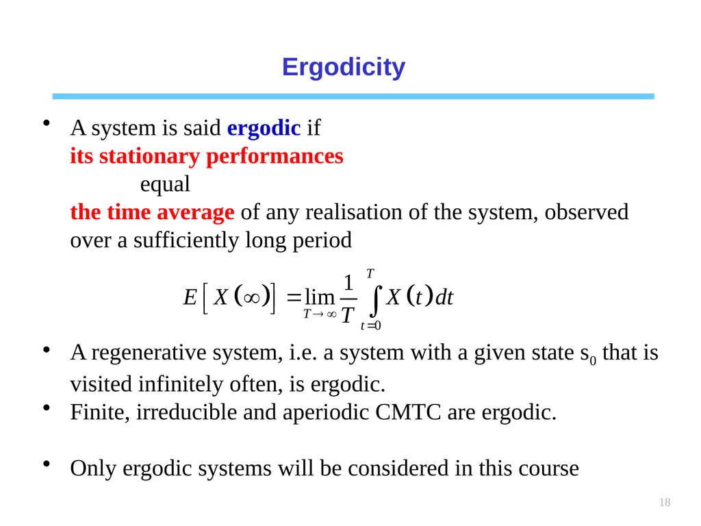
slide18. 18 Ergodicity A system is said ergodic if
its stationary performances
equal
the time average of any realisation of the system, observed over a sufficiently long period

A regenerative system, i.e. a system with a given state s0 that is visited infinitely often, is ergodic.
Finite, irreducible and aperiodic CMTC are ergodic.

Only ergodic systems will be considered in this course<br>
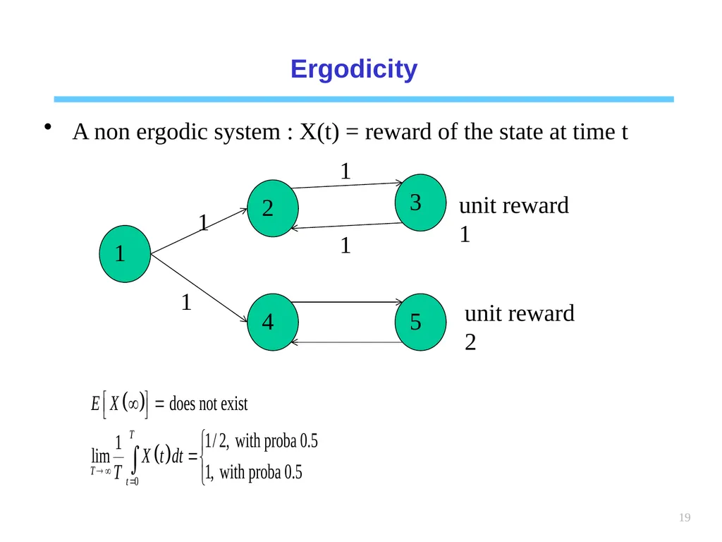
slide19. 19 Ergodicity A non ergodic system : X(t) = reward of the state at time t 1 2 3 4 5 1 1 1 1 unit reward 1 unit reward 2<br>
slide20. 20 Little's law<br>
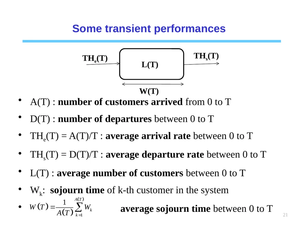
slide21. 21 Some transient performances A(T) : number of customers arrived from 0 to T
D(T) : number of departures between 0 to T
THe(T) = A(T)/T : average arrival rate between 0 to T
THs(T) = D(T)/T : average departure rate between 0 to T
L(T) : average number of customers between 0 to T
Wk: sojourn time of k-th customer in the system
average sojourn time between 0 to T L(T) THe(T) THs(T) W(T)<br>
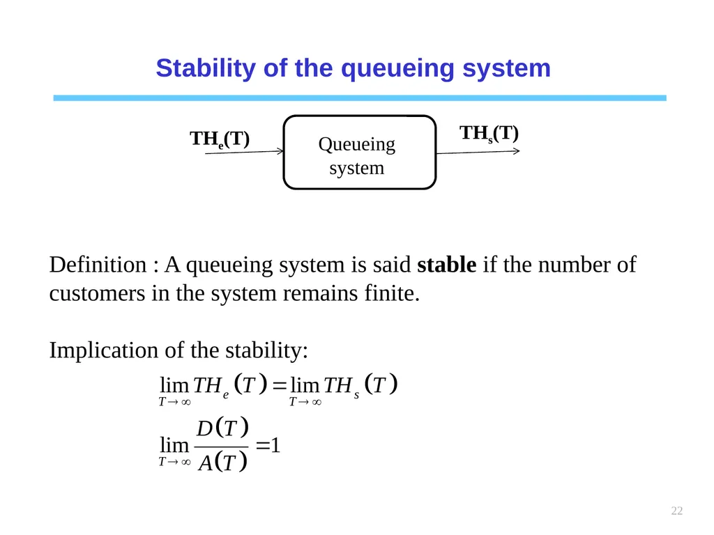
slide22. 22 Stability of the queueing system Definition : A queueing system is said stable if the number of customers in the system remains finite.

Implication of the stability: Queueing system THe(T) THs(T)<br>
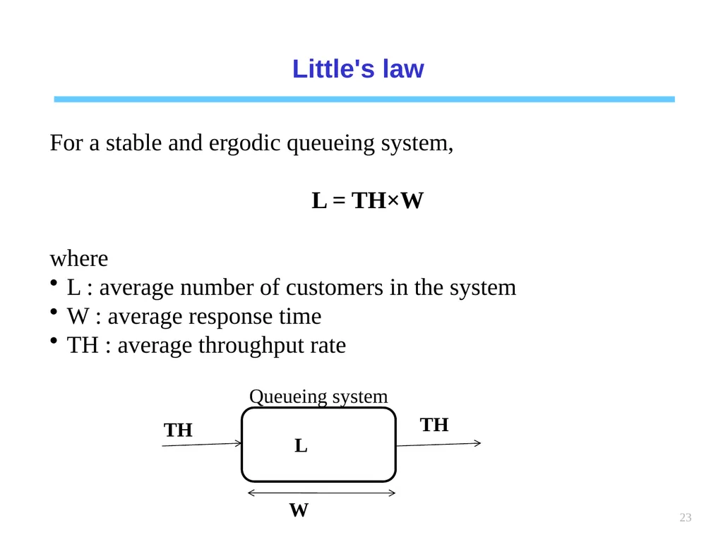
slide23. 23 Little's law For a stable and ergodic queueing system,

L = TH×W

where
L : average number of customers in the system
W : average response time
TH : average throughput rate Queueing system L TH TH W<br>
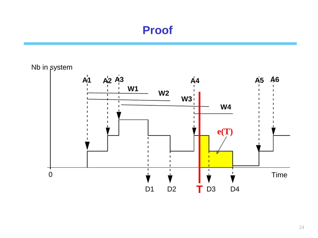
slide24. 24 Proof e(T)<br>
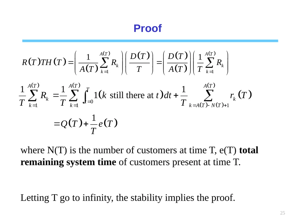
slide25. 25 Proof where N(T) is the number of customers at time T, e(T) total remaining system time of customers present at time T.

Letting T go to infinity, the stability implies the proof.<br>
slide26. 26 Single stage queueing systems<br>
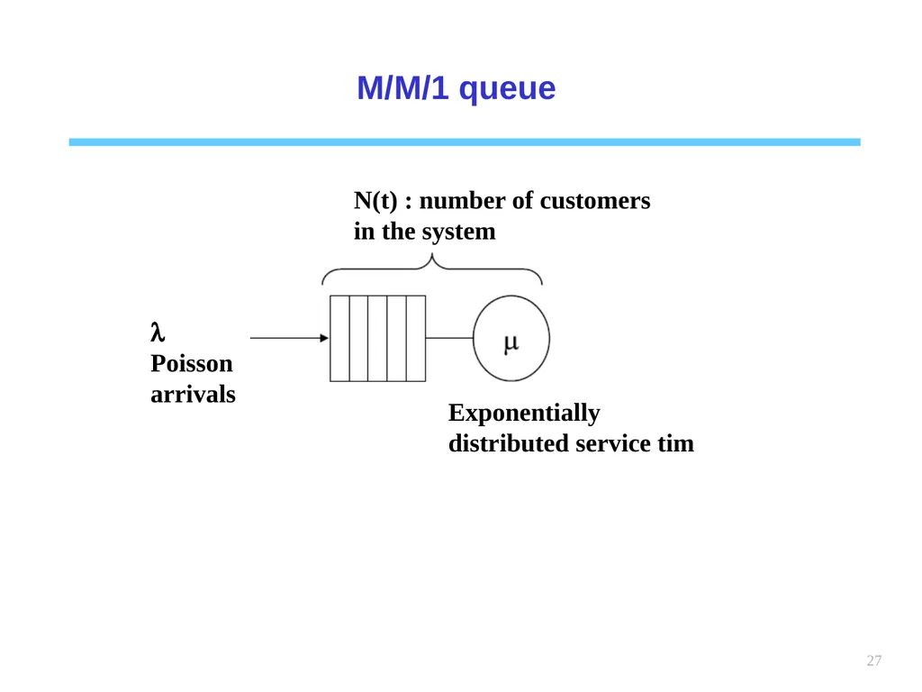
slide27. 27 M/M/1 queue N(t) : number of customers in the system Exponentially distributed service tim l
Poisson arrivals<br>
slide28. 28 Stability condition of M/M/1 queue The M/M/1 queue is stable iff
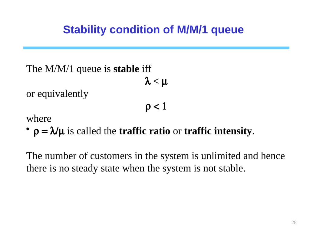
l < m
or equivalently
r < 1
where
r = l/m is called the traffic ratio or traffic intensity.

The number of customers in the system is unlimited and hence there is no steady state when the system is not stable.<br>
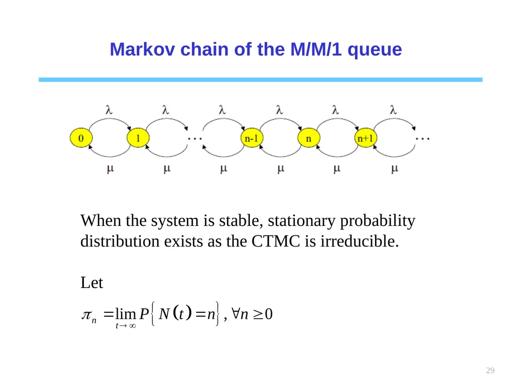
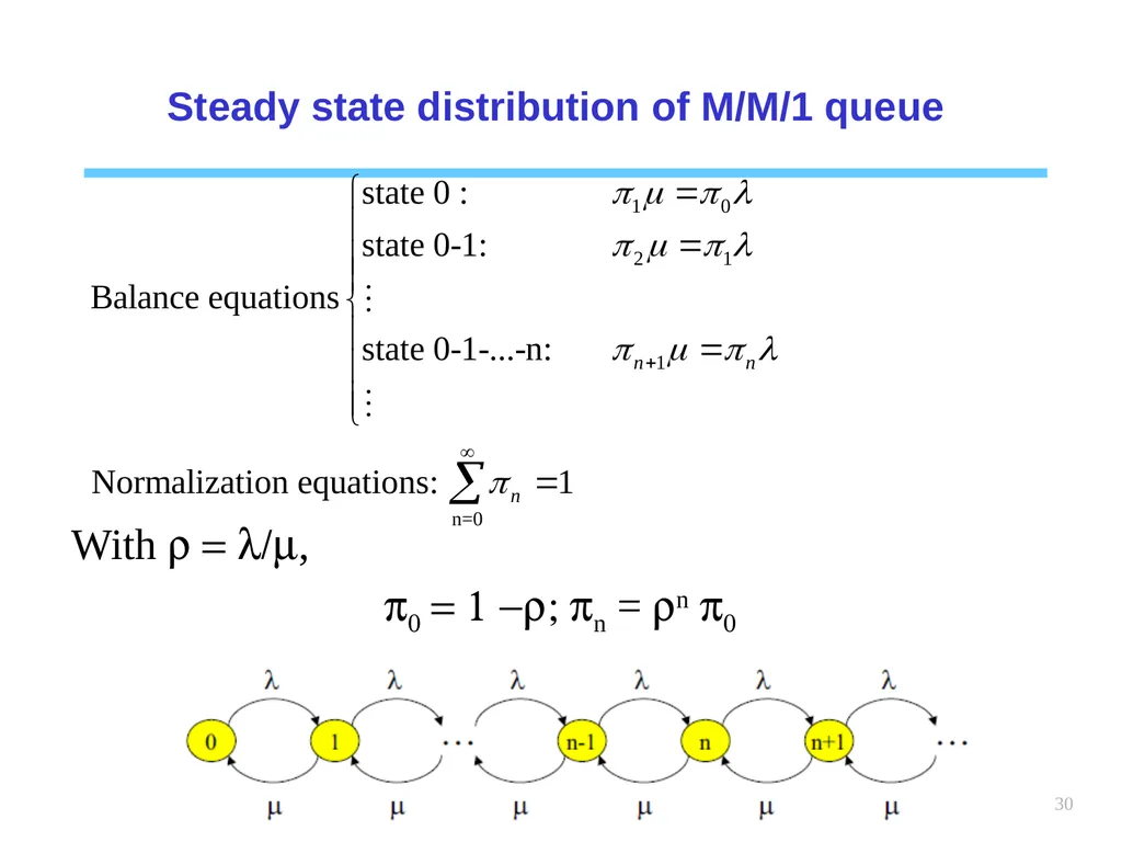
slide29. 29 Markov chain of the M/M/1 queue When the system is stable, stationary probability distribution exists as the CTMC is irreducible.

Let<br>
slide30. 30 Steady state distribution of M/M/1 queue With r = l/m,
p0 = 1 -r; pn = rn p0<br>
slide31. 31 Performance measures of M/M/1 queue
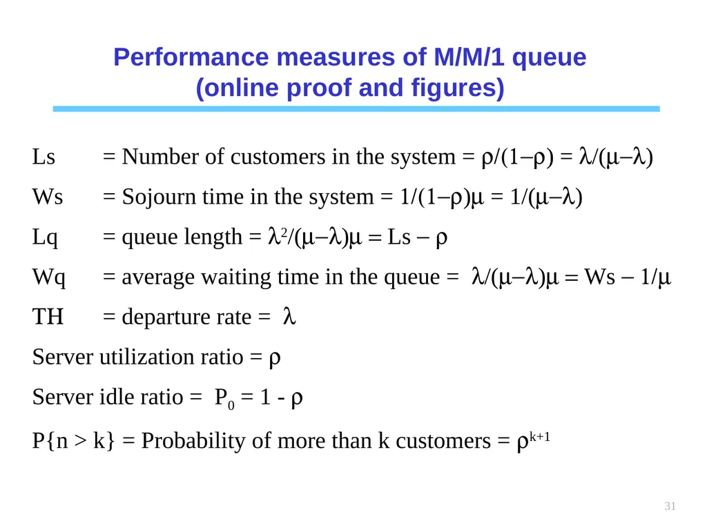
(online proof and figures) Ls = Number of customers in the system = r/(1-r) = l/(m-l)
Ws = Sojourn time in the system = 1/(1-r)m = 1/(m-l)
Lq = queue length = l2/(m-l)m = Ls - r
Wq = average waiting time in the queue = l/(m-l)m = Ws - 1/m
TH = departure rate = l
Server utilization ratio = r
Server idle ratio = P0 = 1 - r
P{n > k} = Probability of more than k customers = rk+1<br>
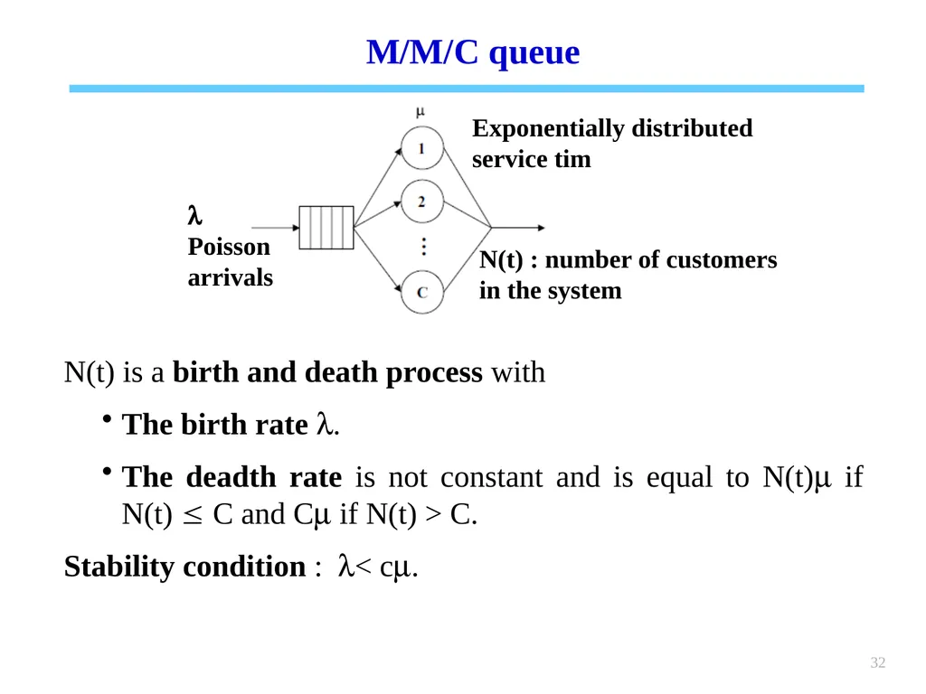
slide32. 32 M/M/C queue N(t) is a birth and death process with
The birth rate l.
The deadth rate is not constant and is equal to N(t)m if N(t)  C and Cm if N(t) > C.
Stability condition : l< cm. N(t) : number of customers in the system Exponentially distributed service tim l
Poisson arrivals<br>
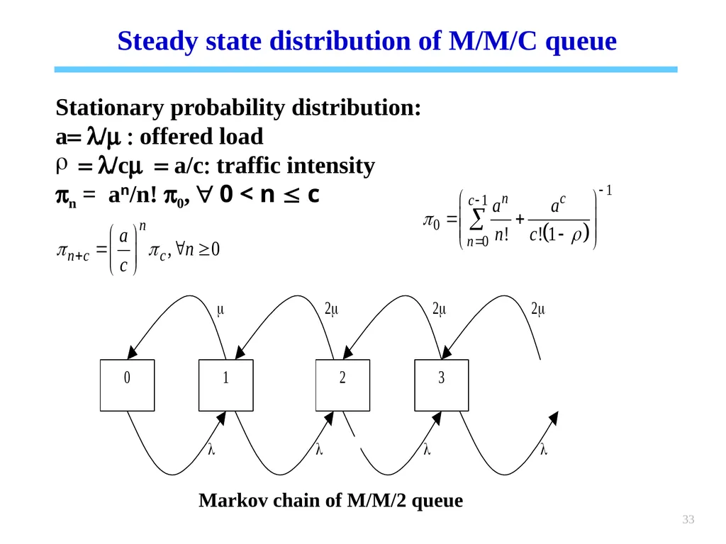
slide33. 33 Steady state distribution of M/M/C queue Markov chain of M/M/2 queue Stationary probability distribution:
a= l/m : offered load
= l/cm = a/c: traffic intensity
pn = an/n! p0, " 0 < n  c<br>
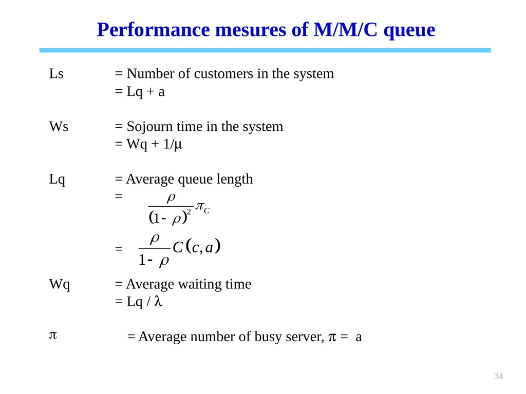
slide34. 34 Performance mesures of M/M/C queue Ls = Number of customers in the system
= Lq + a

Ws = Sojourn time in the system
= Wq + 1/m

Lq = Average queue length
=

=

Wq = Average waiting time
= Lq / l

= Average number of busy server, p = a<br>
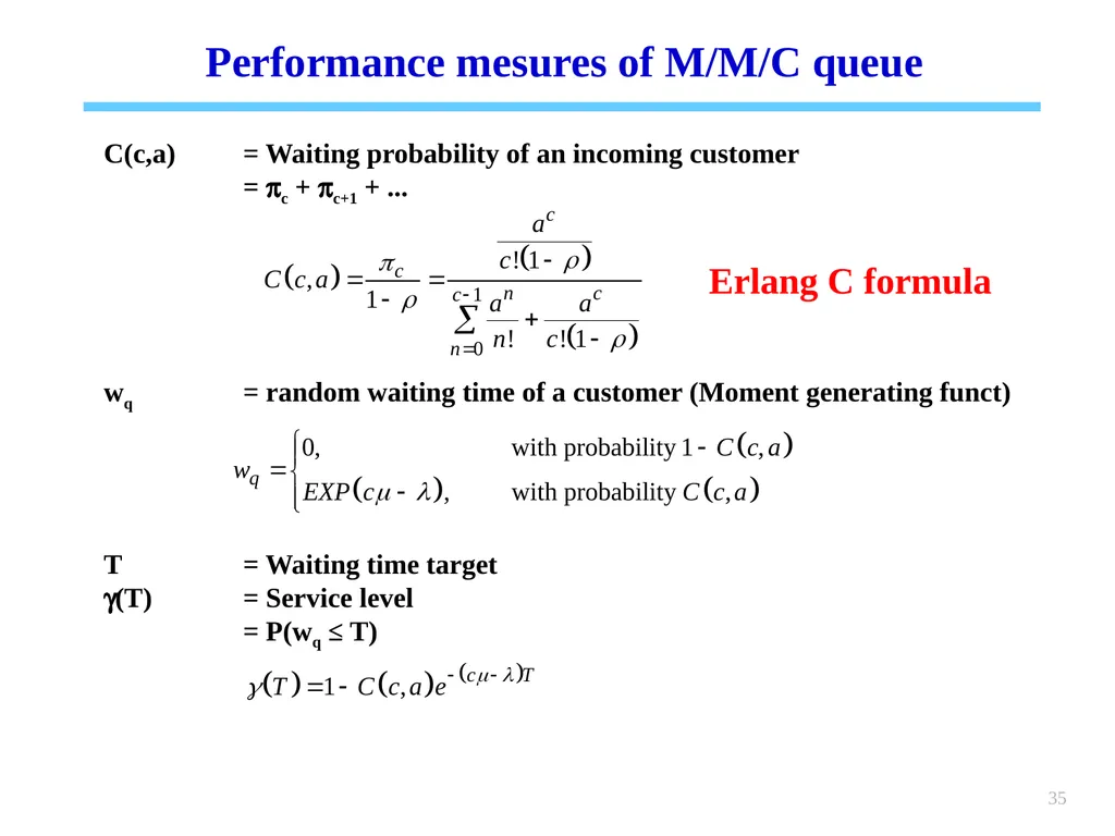
slide35. 35 Performance mesures of M/M/C queue C(c,a) = Waiting probability of an incoming customer
= pc + pc+1 + ...


wq = random waiting time of a customer (Moment generating funct)

T = Waiting time target
g(T) = Service level
= P(wq ≤ T) Erlang C formula<br>
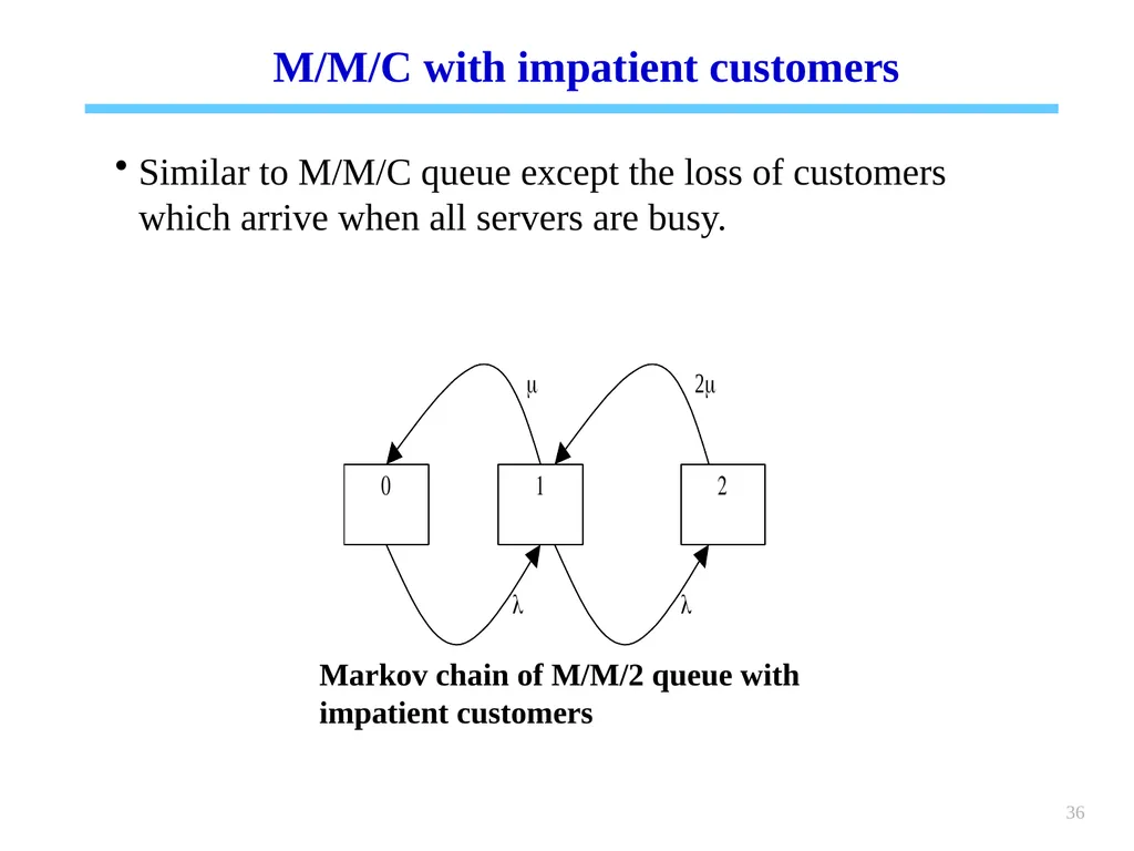
slide36. 36 M/M/C with impatient customers Similar to M/M/C queue except the loss of customers which arrive when all servers are busy. Markov chain of M/M/2 queue with impatient customers<br>
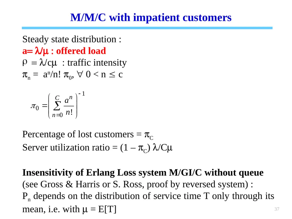
slide37. 37 M/M/C with impatient customers Steady state distribution :
a= l/m : offered load
= l/cm : traffic intensity
pn = an/n! p0, " 0 < n  c

Percentage of lost customers = pC
Server utilization ratio = (1 – pC) l/Cm

Insensitivity of Erlang Loss system M/GI/C without queue
(see Gross & Harris or S. Ross, proof by reversed system) :
Pn depends on the distribution of service time T only through its mean, i.e. with m = E[T]<br>
slide38. M/M/C with impatient customers Erlag loss function or Erlang B formula
= Percentage of lost customers or overflow probability

Accepted load<br>
slide39. M/M/C with impatient customers (optional) Normal approximation for staffing Erlang Loss systems

Condition: high offered load (a > 4) and high targeted service level

N(t) = number of patients : approximately normally distributed

E[N(t)]  a

In M/M/∞ system, N(t) =d POISSON(a), i.e. E[N(t)] = a, Var[N(t)] = a

Square-Root-Staffing-Formula for a delay probability a Where F is the cdf of the standard normal distribution<br>
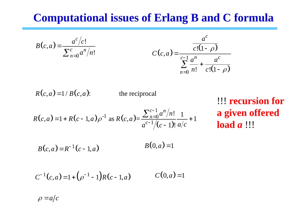
slide40. Computational issues of Erlang B and C formula !!! recursion for a given offered load a !!!<br>
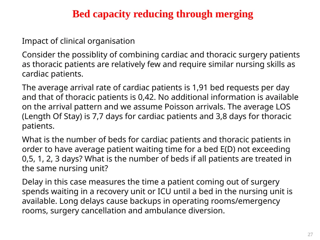
slide41. 27 Impact of clinical organisation
Consider the possiblity of combining cardiac and thoracic surgery patients as thoracic patients are relatively few and require similar nursing skills as cardiac patients.
The average arrival rate of cardiac patients is 1,91 bed requests per day and that of thoracic patients is 0,42. No additional information is available on the arrival pattern and we assume Poisson arrivals. The average LOS (Length Of Stay) is 7,7 days for cardiac patients and 3,8 days for thoracic patients.
What is the number of beds for cardiac patients and thoracic patients in order to have average patient waiting time for a bed E(D) not exceeding 0,5, 1, 2, 3 days? What is the number of beds if all patients are treated in the same nursing unit?
Delay in this case measures the time a patient coming out of surgery spends waiting in a recovery unit or ICU until a bed in the nursing unit is available. Long delays cause backups in operating rooms/emergency rooms, surgery cancellation and ambulance diversion. Bed capacity reducing through merging<br>
slide42. 42 Queueing networks<br>
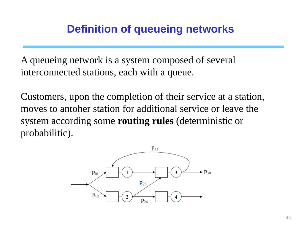
slide43. 43 Definition of queueing networks A queueing network is a system composed of several interconnected stations, each with a queue.

Customers, upon the completion of their service at a station, moves to antoher station for additional service or leave the system according some routing rules (deterministic or probabilitic).<br>
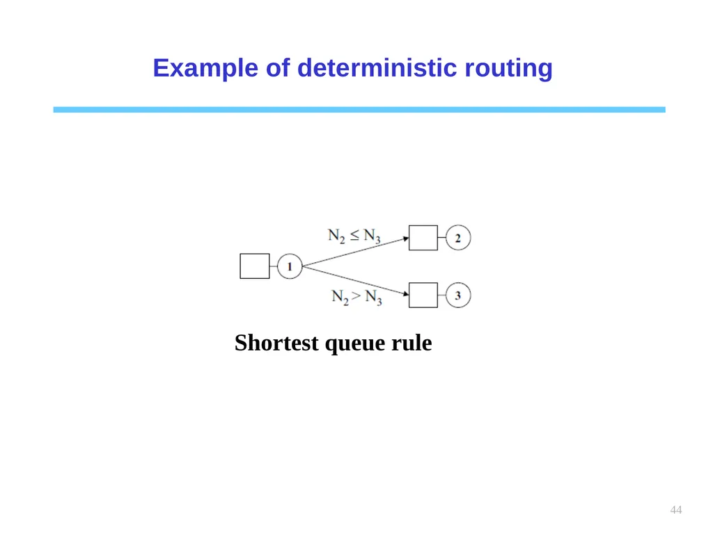
slide44. 44 Example of deterministic routing Shortest queue rule<br>
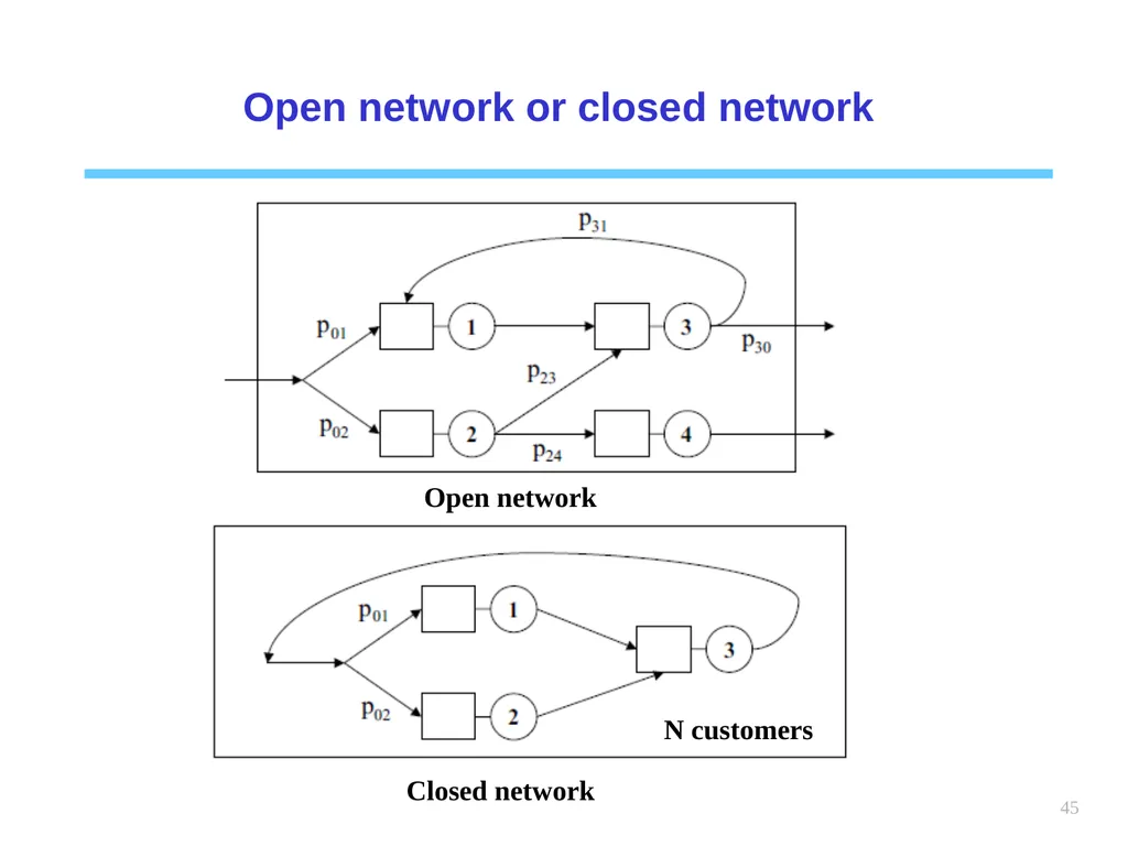
slide45. 45 Open network or closed network<br>
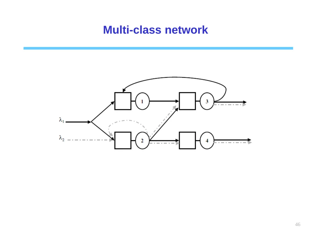
slide46. 46 Multi-class network<br>
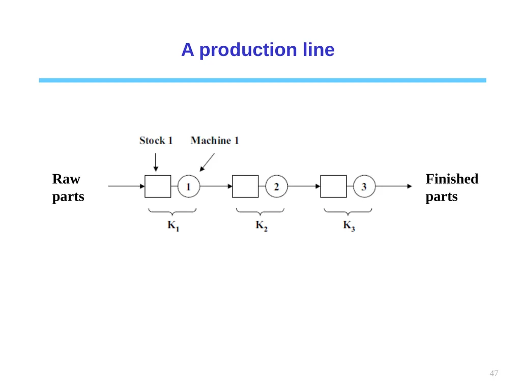
slide47. 47 A production line Raw parts Finished parts<br>
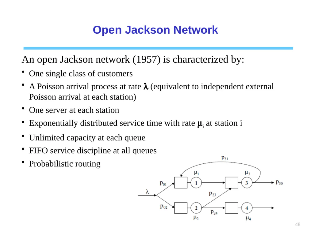
slide48. 48 Open Jackson Network An open Jackson network (1957) is characterized by:
One single class of customers
A Poisson arrival process at rate l (equivalent to independent external Poisson arrival at each station)
One server at each station
Exponentially distributed service time with rate mi at station i
Unlimited capacity at each queue
FIFO service discipline at all queues
Probabilistic routing<br>
slide49. 49 Open Jackson Network
routing pij (i ≠0 and j≠ 0) : probability of moving to station j after service at station i
p0i : probability of an arriving customer joining station i
pi0 : probability of a customer leaving the system after service at station i<br>
slide50. 50 Open Jackson Network
stability condition Let li be the customer arrival rate at station i, for i = 1, ..., M where M is the number of stations.
The system is stable if all stations are stable, i.e.
li < mi, "i = 1, ..., M

Consider also ei the average number of visits to station i for each arriving customer:
ei = li/l<br>
slide51. 51 Open Jackson Network
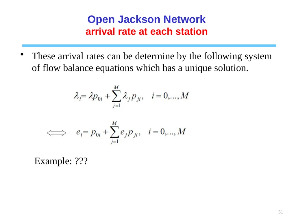
arrival rate at each station These arrival rates can be determine by the following system of flow balance equations which has a unique solution. Example: ???<br>
slide52. 52 Open Jackson Network
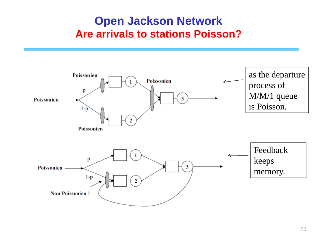
Are arrivals to stations Poisson? as the departure process of M/M/1 queue is Poisson. Feedback keeps memory.<br>
slide53. 53 Open Jackson Network
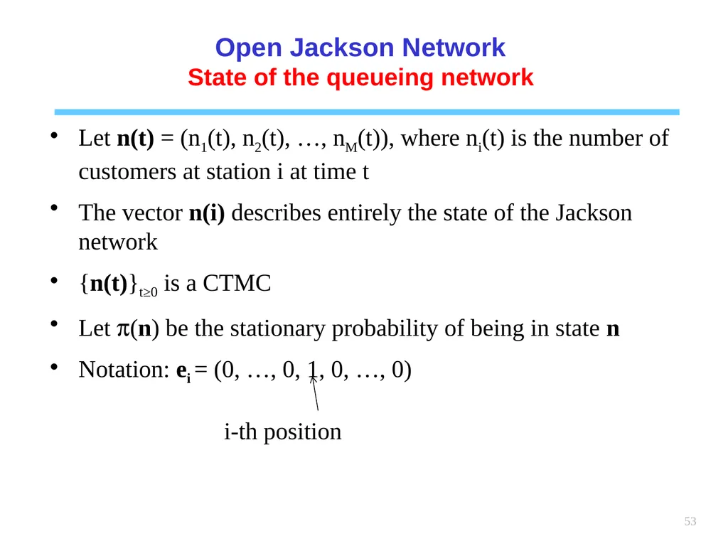
State of the queueing network Let n(t) = (n1(t), n2(t), …, nM(t)), where ni(t) is the number of customers at station i at time t
The vector n(i) describes entirely the state of the Jackson network
{n(t)}t≥0 is a CTMC
Let p(n) be the stationary probability of being in state n
Notation: ei = (0, …, 0, 1, 0, …, 0)

i-th position<br>
slide54. 54 Open Jackson Network
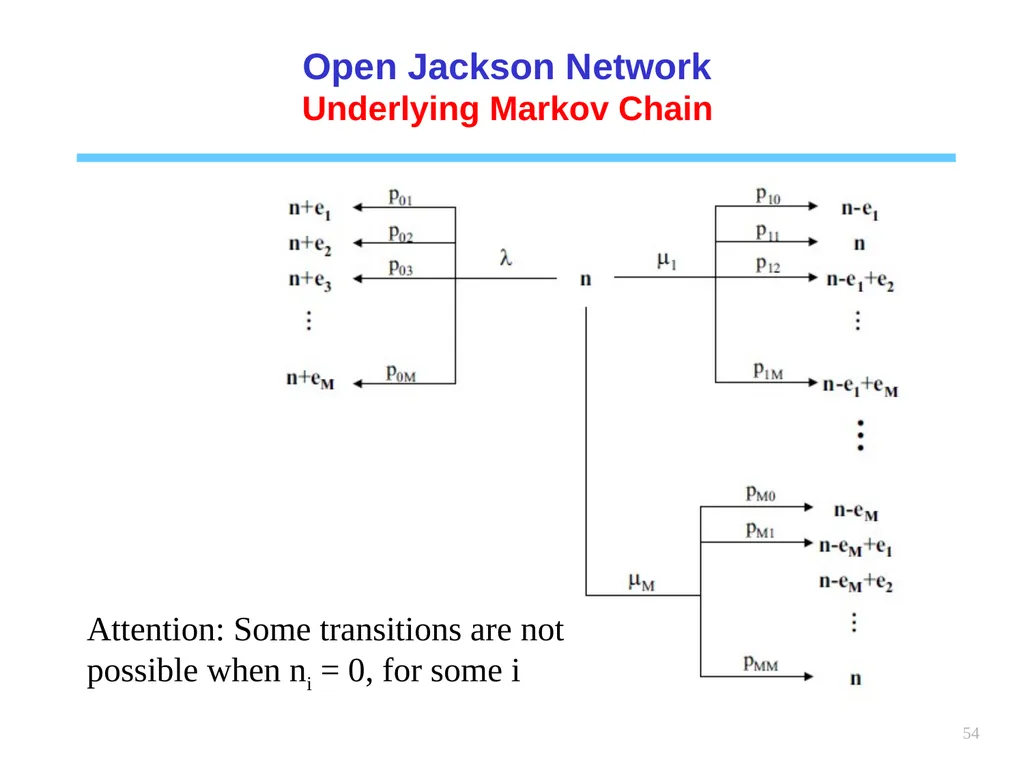
Underlying Markov Chain Attention: Some transitions are not possible when ni = 0, for some i<br>
slide55. 55 Open Jackson Network
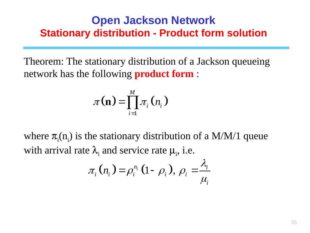
Stationary distribution - Product form solution Theorem: The stationary distribution of a Jackson queueing network has the following product form :

where pi(ni) is the stationary distribution of a M/M/1 queue with arrival rate li and service rate mi, i.e.<br>
slide56. 56 Open Jackson Network
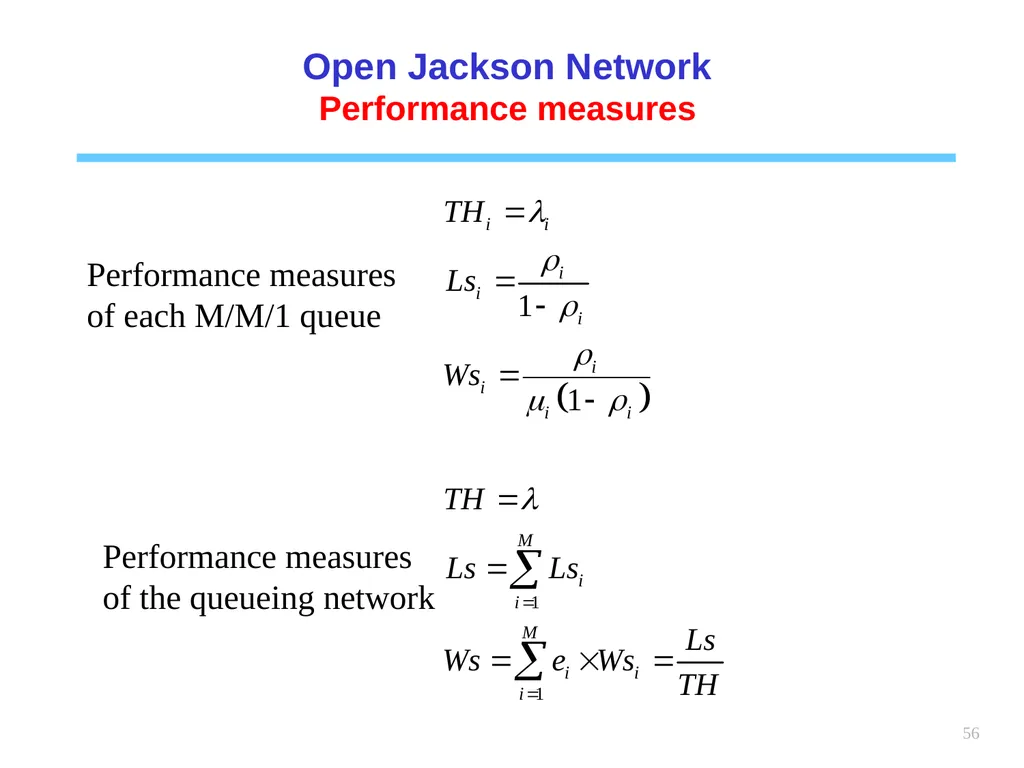
Performance measures Performance measures of each M/M/1 queue Performance measures of the queueing network<br>
slide57. 57 Open Jackson Network
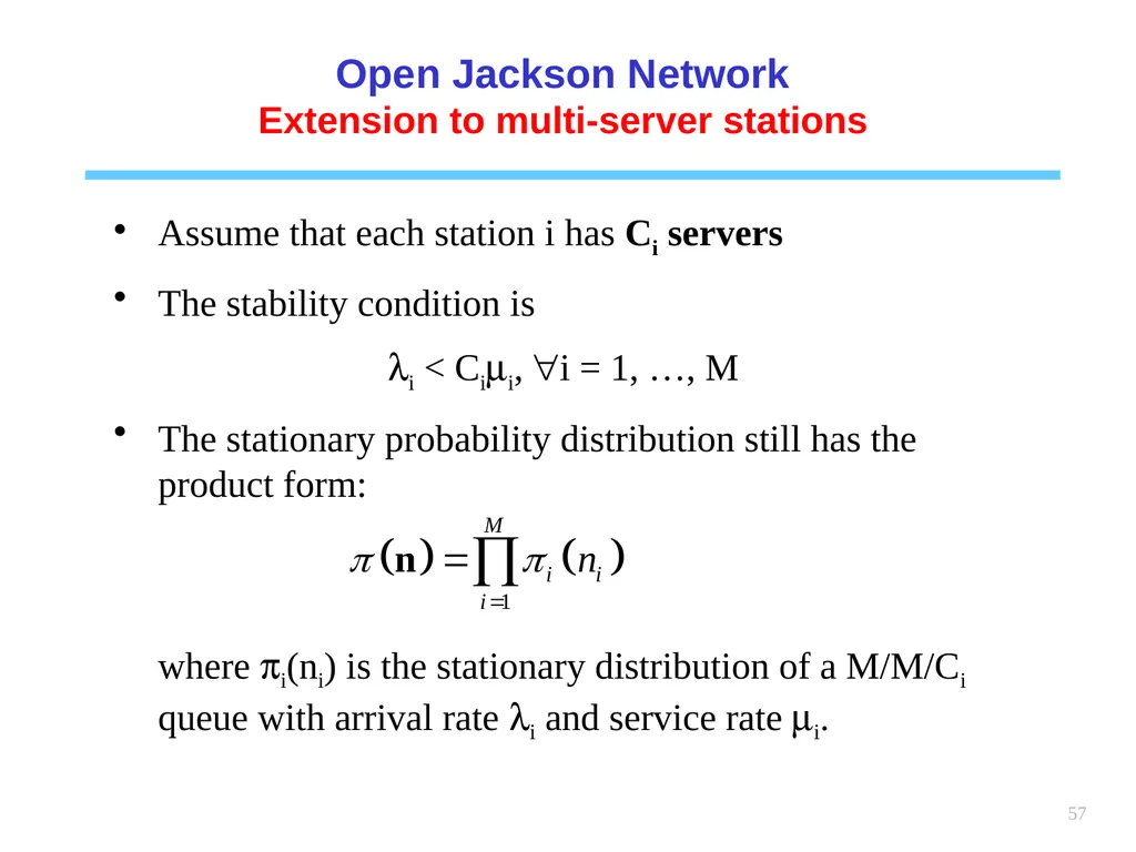
Extension to multi-server stations Assume that each station i has Ci servers
The stability condition is
li < Cimi, "i = 1, …, M
The stationary probability distribution still has the product form:

where pi(ni) is the stationary distribution of a M/M/Ci queue with arrival rate li and service rate mi.<br>
slide58. 58 Open Jackson Network
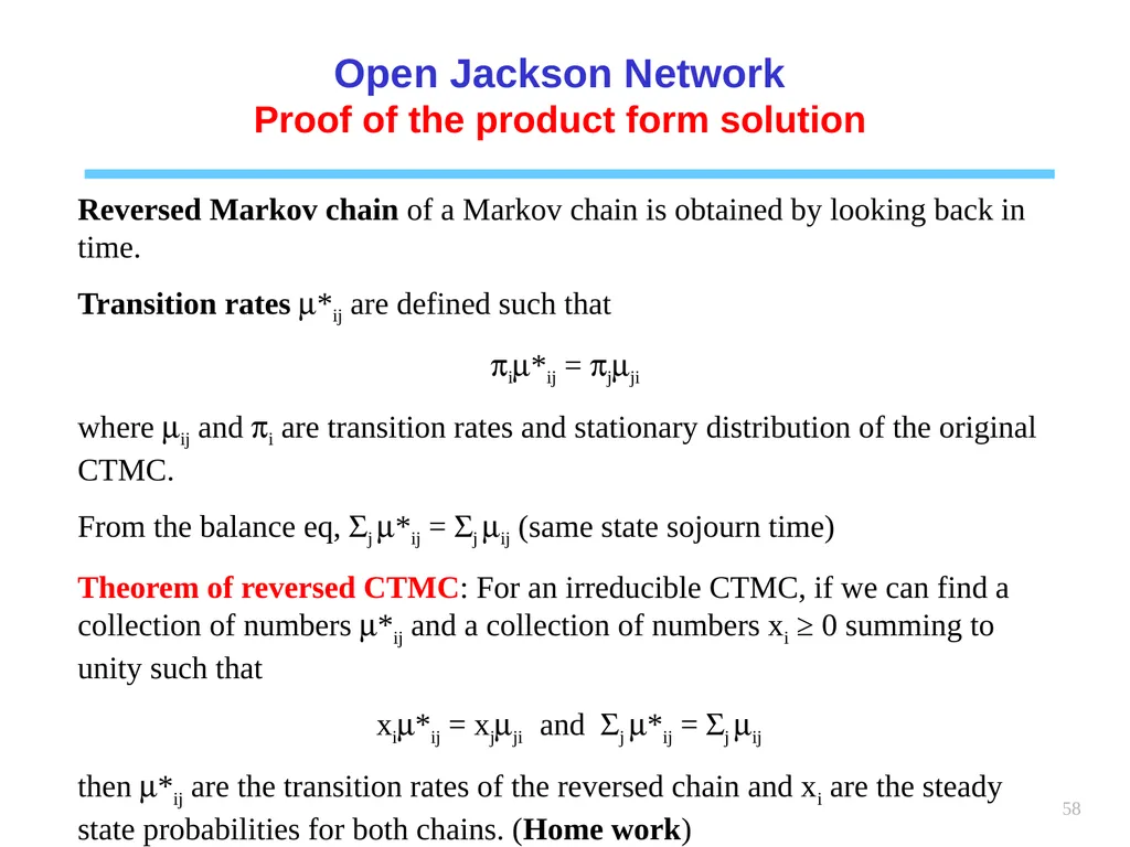
Proof of the product form solution Reversed Markov chain of a Markov chain is obtained by looking back in time.
Transition rates m*ij are defined such that
pim*ij = pjmji
where mij and pi are transition rates and stationary distribution of the original CTMC.
From the balance eq, Sj m*ij = Sj mij (same state sojourn time)
Theorem of reversed CTMC: For an irreducible CTMC, if we can find a collection of numbers m*ij and a collection of numbers xi ≥ 0 summing to unity such that
xim*ij = xjmji and Sj m*ij = Sj mij
then m*ij are the transition rates of the reversed chain and xi are the steady state probabilities for both chains. (Home work)<br>
slide59. 59 Open Jackson Network
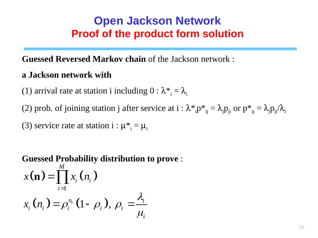
Proof of the product form solution Guessed Reversed Markov chain of the Jackson network :
a Jackson network with
(1) arrival rate at station i including 0 : l*i = li
(2) prob. of joining station j after service at i : l*ip*ij = ljpji or p*ij = ljpji/li
(3) service rate at station i : m*i = mi

Guessed Probability distribution to prove :<br>
slide60. 60 Open Jackson Network
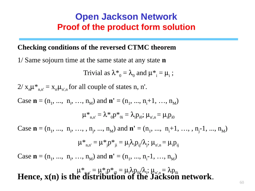
Proof of the product form solution Checking conditions of the reversed CTMC theorem
1/ Same sojourn time at the same state at any state n
Trivial as l*0 = l0 and m*i = mi ;
2/ xnm*n,n' = xn'mn',n for all couple of states n, n'.
Case n = (n1, ..., ni, …, nM) and n' = (n1, ..., ni+1, …, nM)
m*n,n' = l*0p*0i = lipi0; mn',n = mipi0
Case n = (n1, ..., ni, …, , nj, ..., nM) and n' = (n1, ..., ni+1, …, , nj-1, ..., nM)
m*n,n' = m*jp*ji = mjlipij/lj; mn',n = mipij
Case n = (n1, ..., ni, …, nM) and n' = (n1, ..., ni-1, …, nM)
m*n,n' = m*ip*i0 = milp0i/li; mn',n = lp0i Hence, x(n) is the distribution of the Jackson network.<br>
slide61. 61 Closed Queuing Network
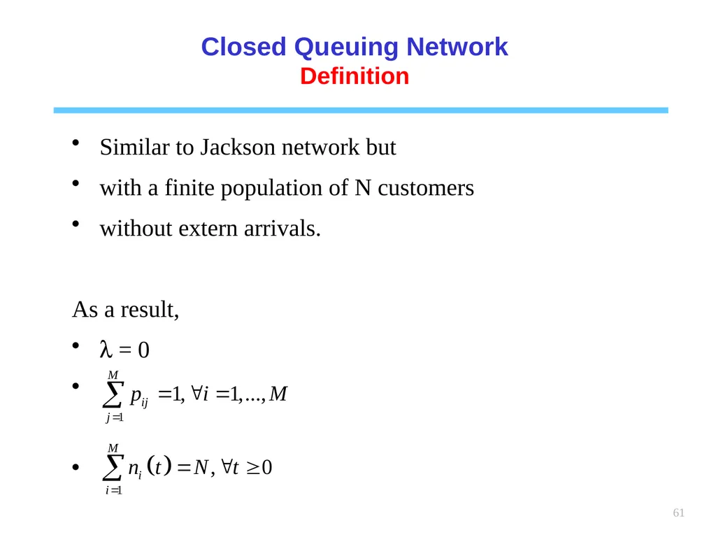
Definition Similar to Jackson network but
with a finite population of N customers
without extern arrivals.

As a result,
l = 0<br>
slide62. 62 Closed Queuing Network
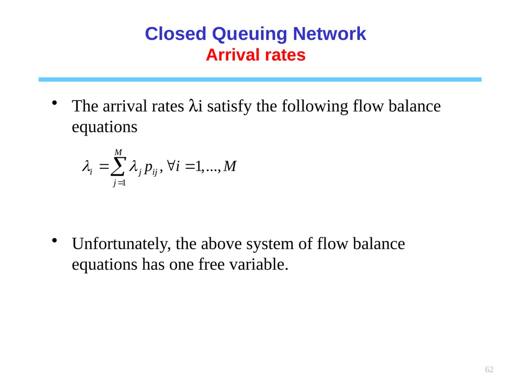
Arrival rates The arrival rates li satisfy the following flow balance equations

Unfortunately, the above system of flow balance equations has one free variable.<br>
slide63. 63 Closed Queuing Network
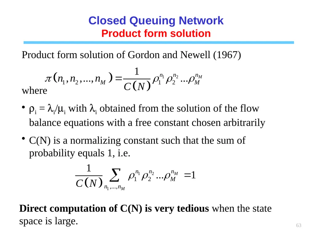
Product form solution Product form solution of Gordon and Newell (1967)

where
ri = li/mi with li obtained from the solution of the flow balance equations with a free constant chosen arbitrarily
C(N) is a normalizing constant such that the sum of probability equals 1, i.e. Direct computation of C(N) is very tedious when the state space is large.<br>
slide64. 64 Closed Queuing Network
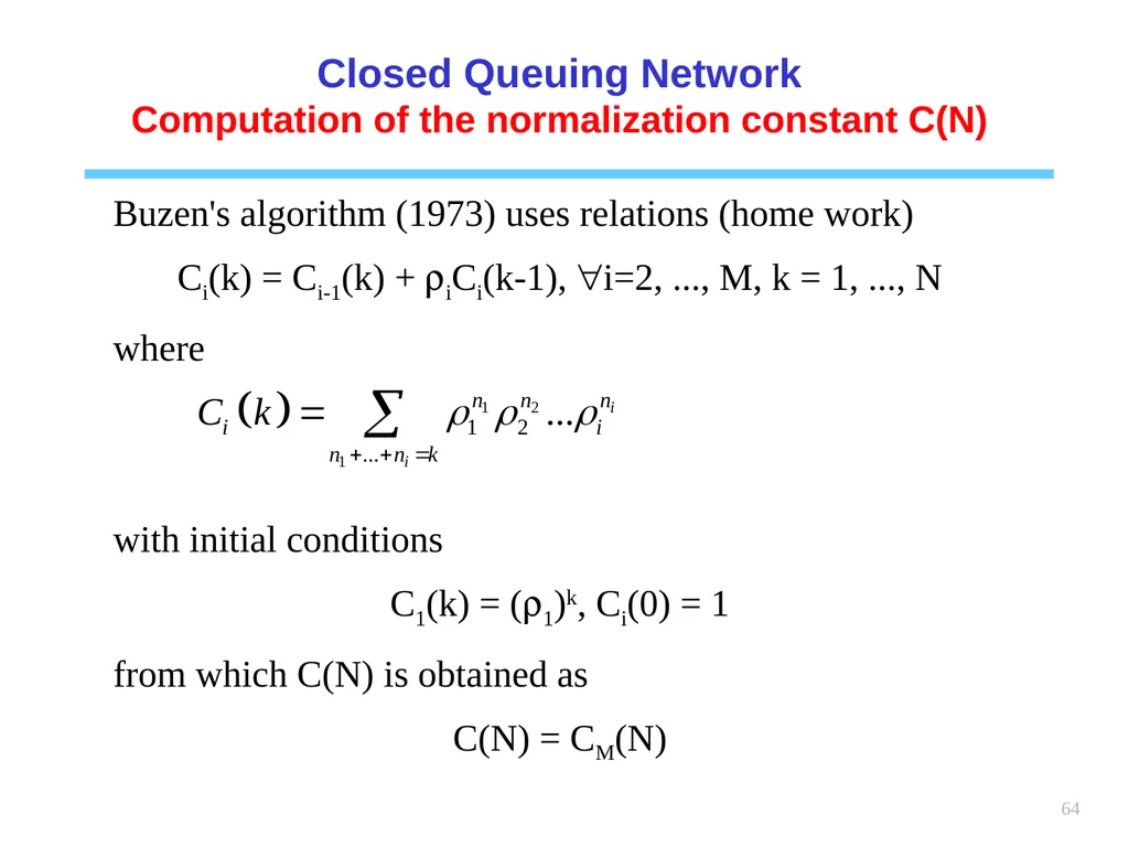
Computation of the normalization constant C(N) Buzen's algorithm (1973) uses relations (home work)
Ci(k) = Ci-1(k) + riCi(k-1), "i=2, ..., M, k = 1, ..., N
where

with initial conditions
C1(k) = (r1)k, Ci(0) = 1
from which C(N) is obtained as
C(N) = CM(N)<br>
slide65. 65 Closed Queuing Network
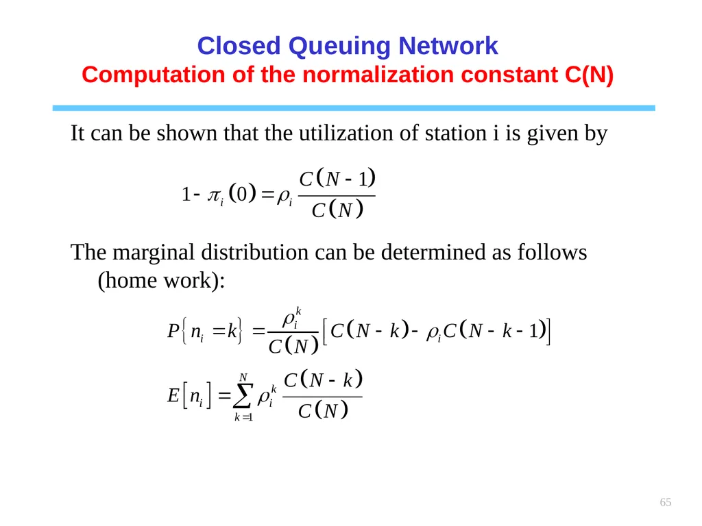
Computation of the normalization constant C(N) It can be shown that the utilization of station i is given by

The marginal distribution can be determined as follows (home work):<br>
slide66. 66 Closed Queuing Network
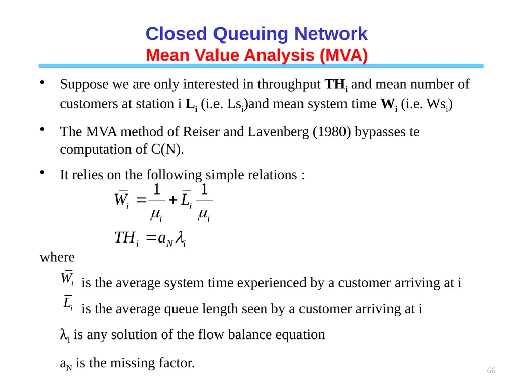
Mean Value Analysis (MVA) Suppose we are only interested in throughput THi and mean number of customers at station i Li (i.e. Lsi)and mean system time Wi (i.e. Wsi)
The MVA method of Reiser and Lavenberg (1980) bypasses te computation of C(N).
It relies on the following simple relations :

where
is the average system time experienced by a customer arriving at i
is the average queue length seen by a customer arriving at i
li is any solution of the flow balance equation
aN is the missing factor.<br>
slide67. 67 Closed Queuing Network
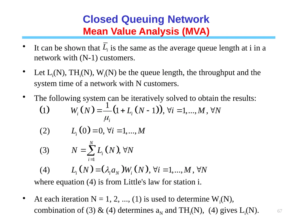
Mean Value Analysis (MVA) It can be shown that is the same as the average queue length at i in a network with (N-1) customers.
Let Li(N), THi(N), Wi(N) be the queue length, the throughput and the system time of a network with N customers.
The following system can be iteratively solved to obtain the results:

where equation (4) is from Little's law for station i.
At each iteration N = 1, 2, ..., (1) is used to determine Wi(N), combination of (3) & (4) determines aN and THi(N), (4) gives Li(N).<br>
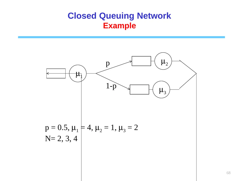
slide68. 68 Closed Queuing Network
Example p 1-p p = 0.5, m1 = 4, m2 = 1, m3 = 2
N= 2, 3, 4<br>
slide69. 69 Non Markovian queueing systems<br>
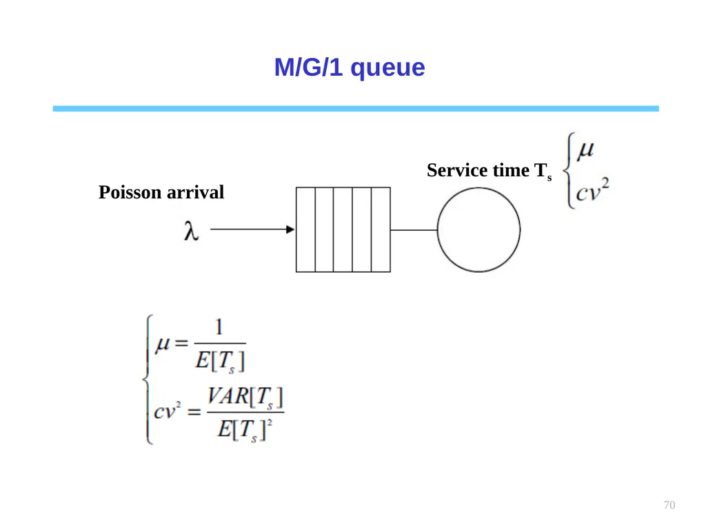
slide70. 70 M/G/1 queue<br>
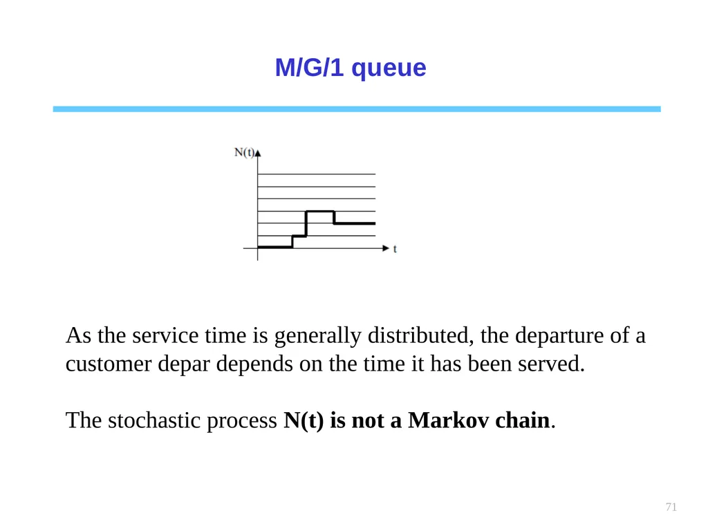
slide71. 71 M/G/1 queue As the service time is generally distributed, the departure of a customer depar depends on the time it has been served.

The stochastic process N(t) is not a Markov chain.<br>
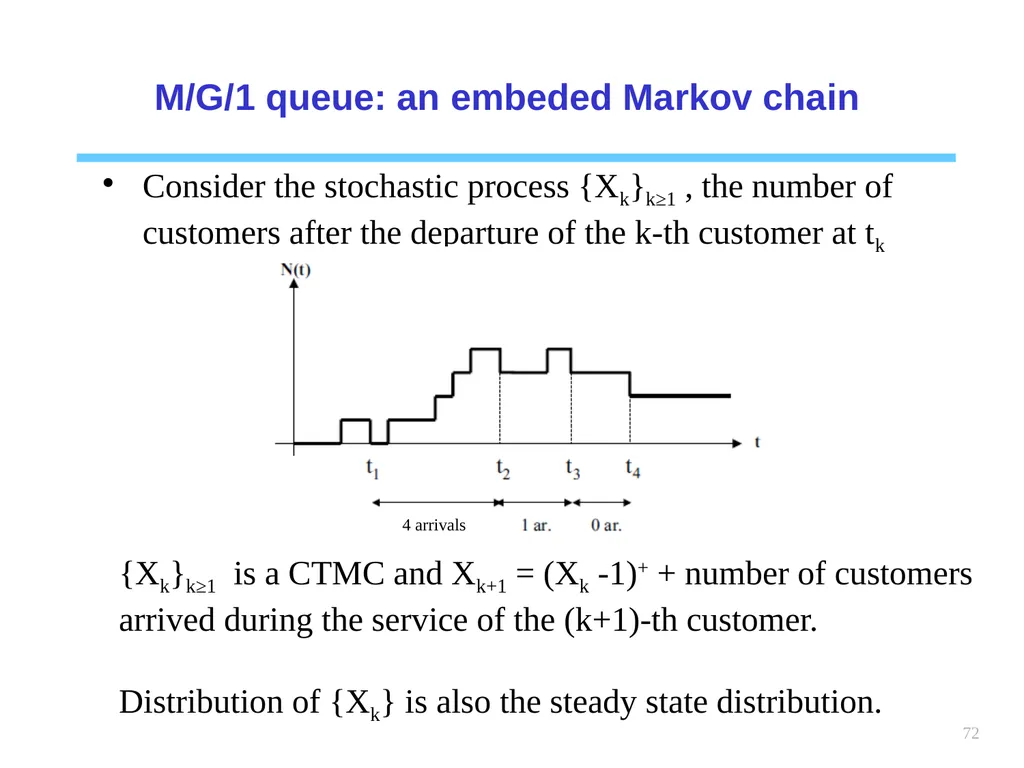
slide72. 72 M/G/1 queue: an embeded Markov chain {Xk}k≥1 is a CTMC and Xk+1 = (Xk -1)+ + number of customers arrived during the service of the (k+1)-th customer.

Distribution of {Xk} is also the steady state distribution. Consider the stochastic process {Xk}k≥1 , the number of customers after the departure of the k-th customer at tk<br>
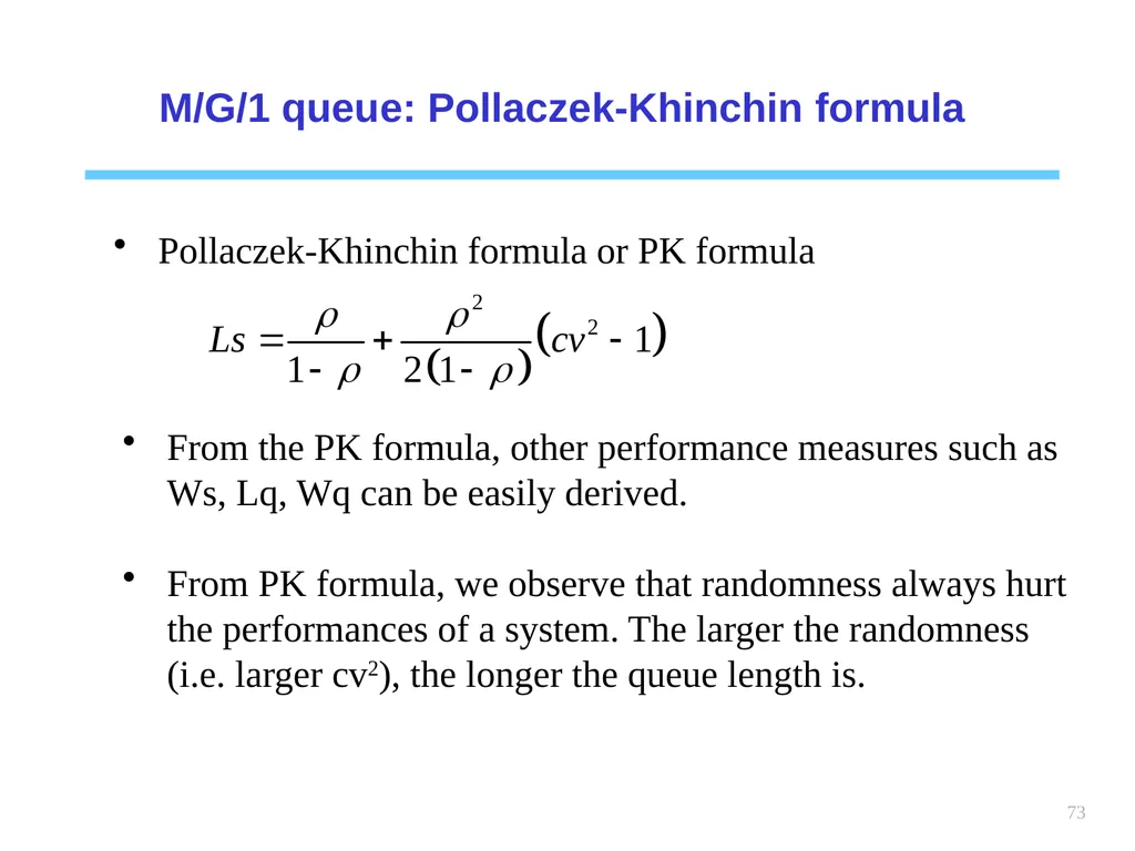
slide73. 73 M/G/1 queue: Pollaczek-Khinchin formula Pollaczek-Khinchin formula or PK formula From the PK formula, other performance measures such as Ws, Lq, Wq can be easily derived.

From PK formula, we observe that randomness always hurt the performances of a system. The larger the randomness (i.e. larger cv2), the longer the queue length is.<br>
slide74. 74 M/G/1 queue: Why it works
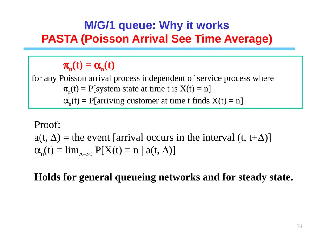
PASTA (Poisson Arrival See Time Average) pn(t) = an(t)
for any Poisson arrival process independent of service process where
pn(t) = P[system state at time t is X(t) = n]
an(t) = P[arriving customer at time t finds X(t) = n] Proof:
a(t, D) = the event [arrival occurs in the interval (t, t+D)]
an(t) = limD->0 P[X(t) = n | a(t, D)]

Holds for general queueing networks and for steady state.<br>
slide75. 75 M/G/1 queue: Why it works
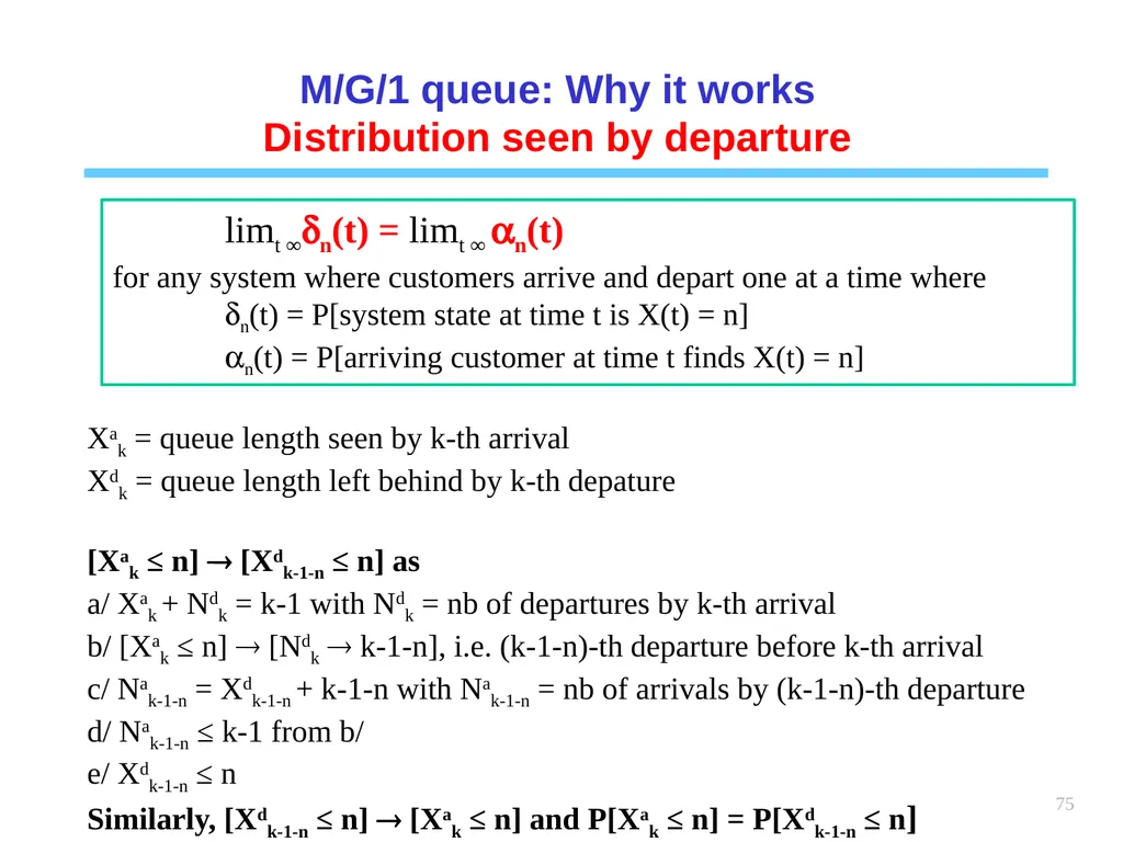
Distribution seen by departure limt∞dn(t) = limt∞ an(t)
for any system where customers arrive and depart one at a time where
dn(t) = P[system state at time t is X(t) = n]
an(t) = P[arriving customer at time t finds X(t) = n] Xak = queue length seen by k-th arrival
Xdk = queue length left behind by k-th depature

[Xak ≤ n]  [Xdk-1-n ≤ n] as
a/ Xak + Ndk = k-1 with Ndk = nb of departures by k-th arrival
b/ [Xak ≤ n]  [Ndk  k-1-n], i.e. (k-1-n)-th departure before k-th arrival
c/ Nak-1-n = Xdk-1-n + k-1-n with Nak-1-n = nb of arrivals by (k-1-n)-th departure
d/ Nak-1-n ≤ k-1 from b/
e/ Xdk-1-n ≤ n
Similarly, [Xdk-1-n ≤ n]  [Xak ≤ n] and P[Xak ≤ n] = P[Xdk-1-n ≤ n]<br>
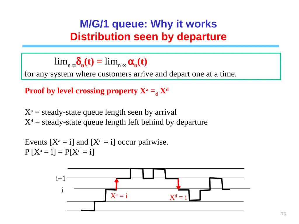
slide76. 76 M/G/1 queue: Why it works
Distribution seen by departure limn∞dn(t) = limn∞ an(t)
for any system where customers arrive and depart one at a time. Proof by level crossing property Xa =d Xd

Xa = steady-state queue length seen by arrival
Xd = steady-state queue length left behind by departure

Events [Xa = i] and [Xd = i] occur pairwise.
P [Xa = i] = P[Xd = i] i i+1 Xa = i Xd = i<br>
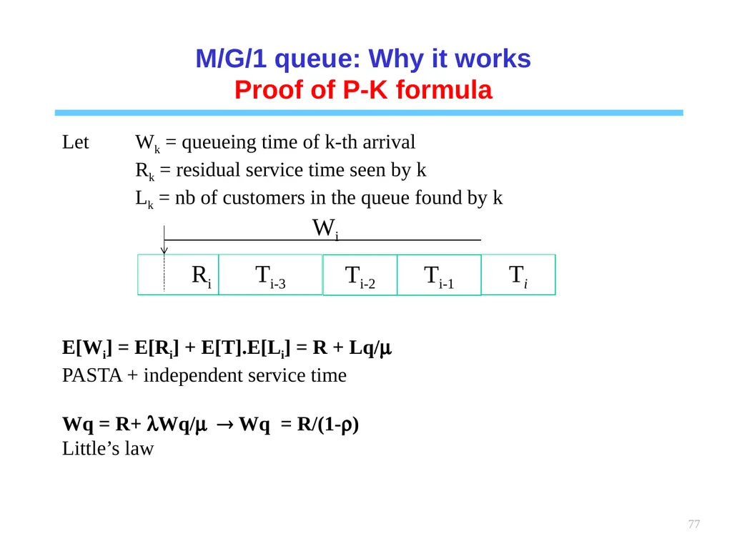
slide77. 77 M/G/1 queue: Why it works
Proof of P-K formula Let Wk = queueing time of k-th arrival
Rk = residual service time seen by k
Lk = nb of customers in the queue found by k

E[Wi] = E[Ri] + E[T].E[Li] = R + Lq/m
PASTA + independent service time

Wq = R+ lWq/m  Wq = R/(1-r)
Little’s law Ri Ti-3 Ti-2 Ti-1 Ti Wi<br>
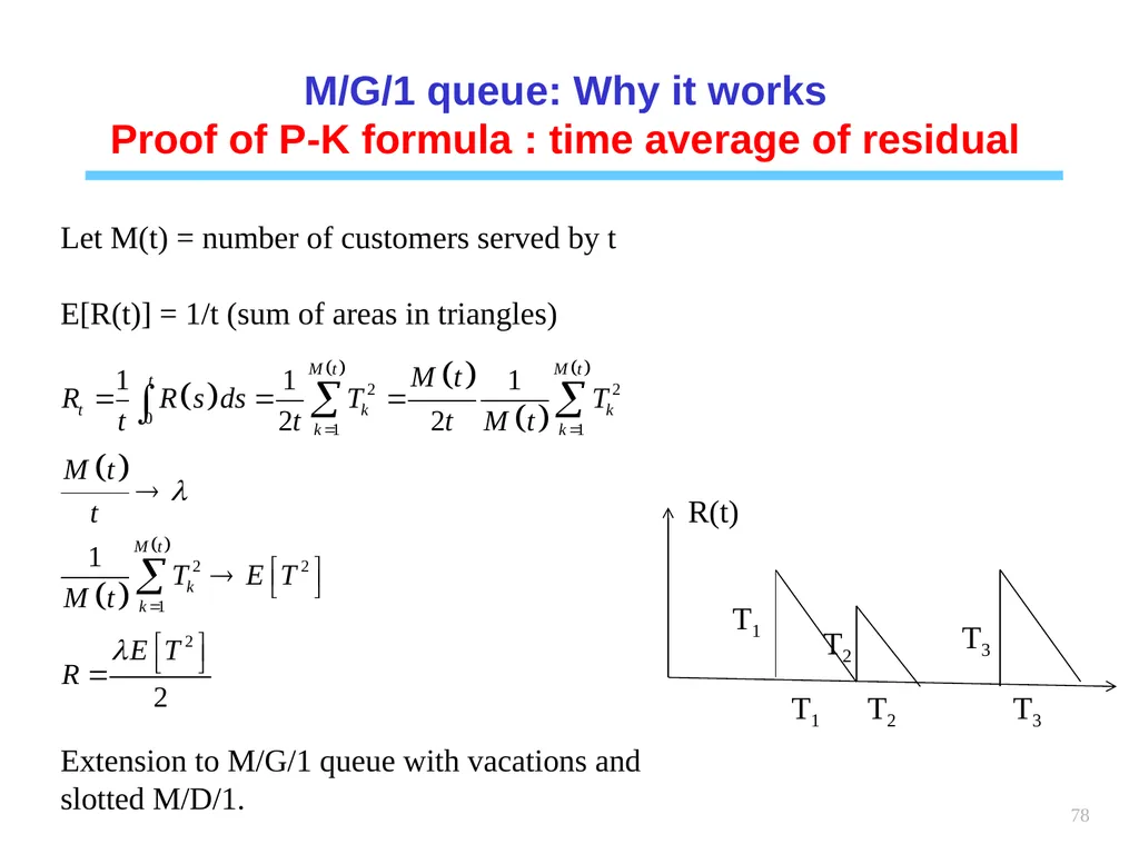
slide78. 78 M/G/1 queue: Why it works
Proof of P-K formula : time average of residual Let M(t) = number of customers served by t

E[R(t)] = 1/t (sum of areas in triangles) T1 T2 T1 T2 T3 T3 R(t) Extension to M/G/1 queue with vacations and slotted M/D/1.<br>
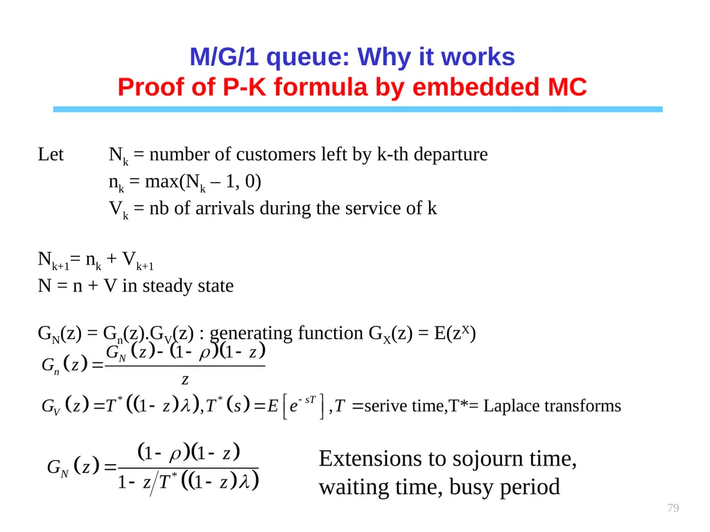
slide79. 79 M/G/1 queue: Why it works
Proof of P-K formula by embedded MC Let Nk = number of customers left by k-th departure
nk = max(Nk – 1, 0)
Vk = nb of arrivals during the service of k

Nk+1= nk + Vk+1
N = n + V in steady state

GN(z) = Gn(z).GV(z) : generating function GX(z) = E(zX) Extensions to sojourn time, waiting time, busy period<br>
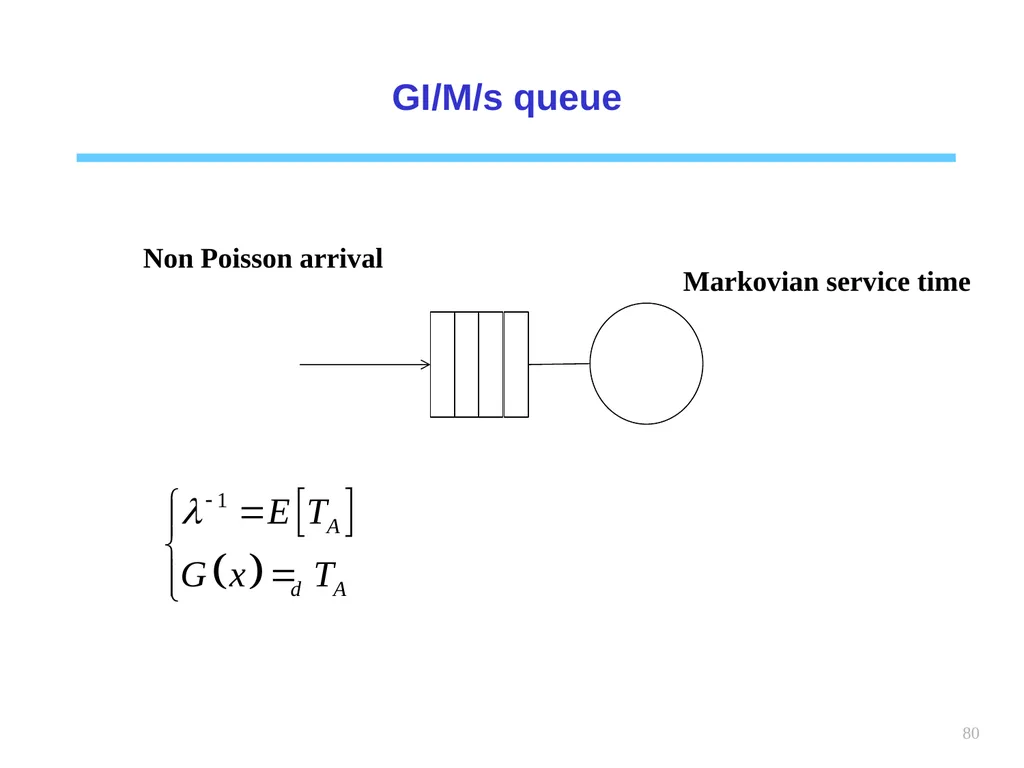
slide80. 80 GI/M/s queue Non Poisson arrival Markovian service time<br>
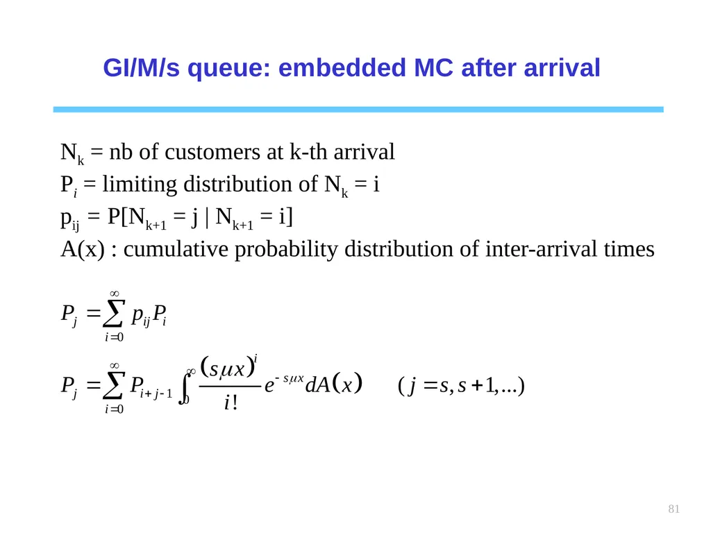
slide81. 81 GI/M/s queue: embedded MC after arrival Nk = nb of customers at k-th arrival
Pi = limiting distribution of Nk = i
pij = P[Nk+1 = j | Nk+1 = i]
A(x) : cumulative probability distribution of inter-arrival times<br>
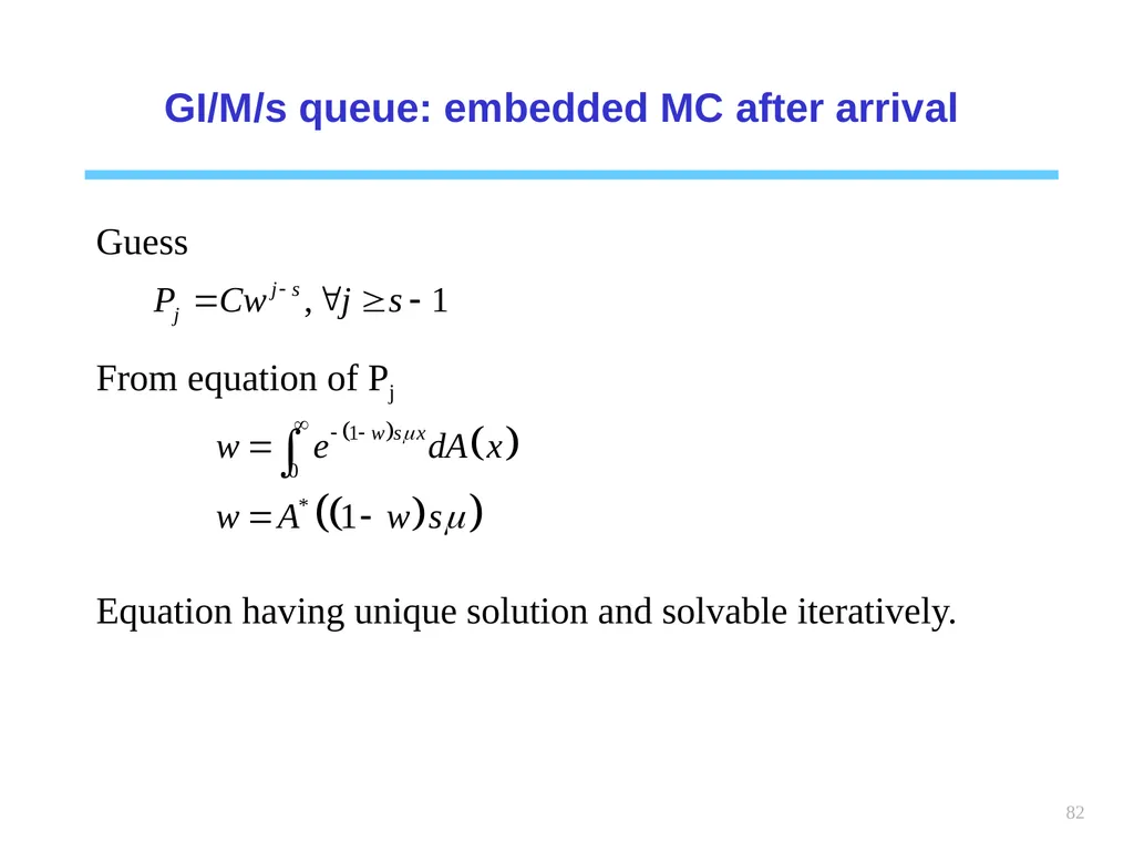
slide82. 82 GI/M/s queue: embedded MC after arrival Guess

From equation of Pj

Equation having unique solution and solvable iteratively.<br>
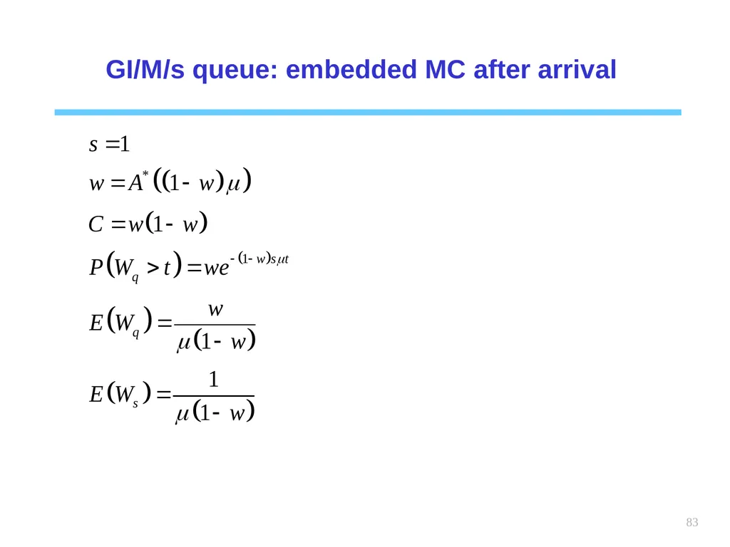
slide83. 83 GI/M/s queue: embedded MC after arrival<br>
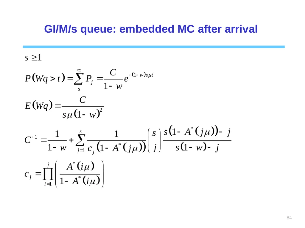
slide84. 84 GI/M/s queue: embedded MC after arrival<br>
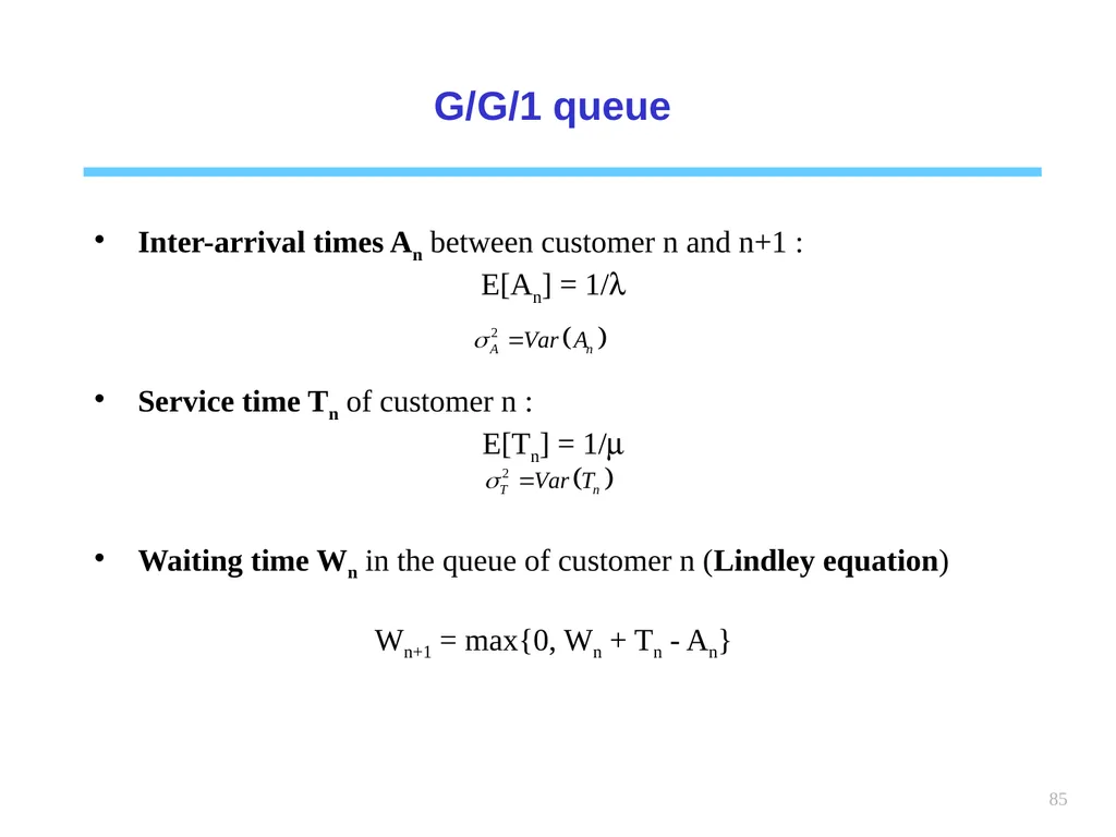
slide85. 85 G/G/1 queue Inter-arrival times An between customer n and n+1 :
E[An] = 1/l

Service time Tn of customer n :
E[Tn] = 1/m

Waiting time Wn in the queue of customer n (Lindley equation)

Wn+1 = max{0, Wn + Tn - An}<br>
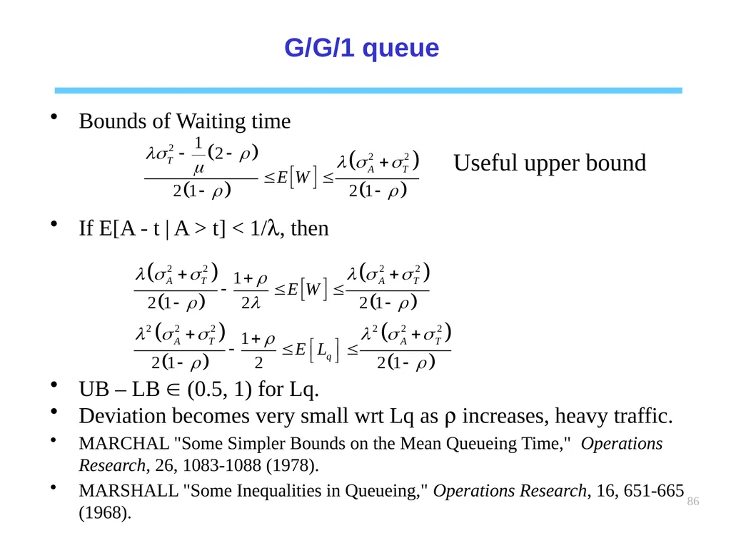
slide86. 86 G/G/1 queue Bounds of Waiting time

If E[A - t | A > t] < 1/l, then

UB – LB  (0.5, 1) for Lq.
Deviation becomes very small wrt Lq as r increases, heavy traffic.
MARCHAL "Some Simpler Bounds on the Mean Queueing Time,"  Operations Research, 26, 1083-1088 (1978).
MARSHALL "Some Inequalities in Queueing," Operations Research, 16, 651-665 (1968). Useful upper bound<br>
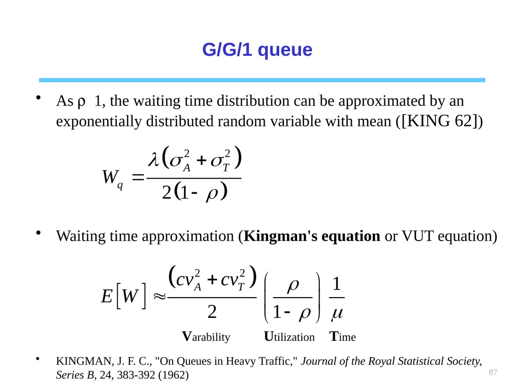
slide87. 87 G/G/1 queue As r 1, the waiting time distribution can be approximated by an exponentially distributed random variable with mean ([KING 62])

Waiting time approximation (Kingman's equation or VUT equation)

KINGMAN, J. F. C., "On Queues in Heavy Traffic," Journal of the Royal Statistical Society, Series B, 24, 383-392 (1962) Varability Utilization Time<br>
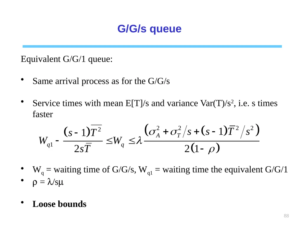
slide88. 88 G/G/s queue Equivalent G/G/1 queue:

Same arrival process as for the G/G/s

Service times with mean E[T]/s and variance Var(T)/s2, i.e. s times faster

Wq = waiting time of G/G/s, Wq1 = waiting time the equivalent G/G/1
r = l/sm

Loose bounds<br>
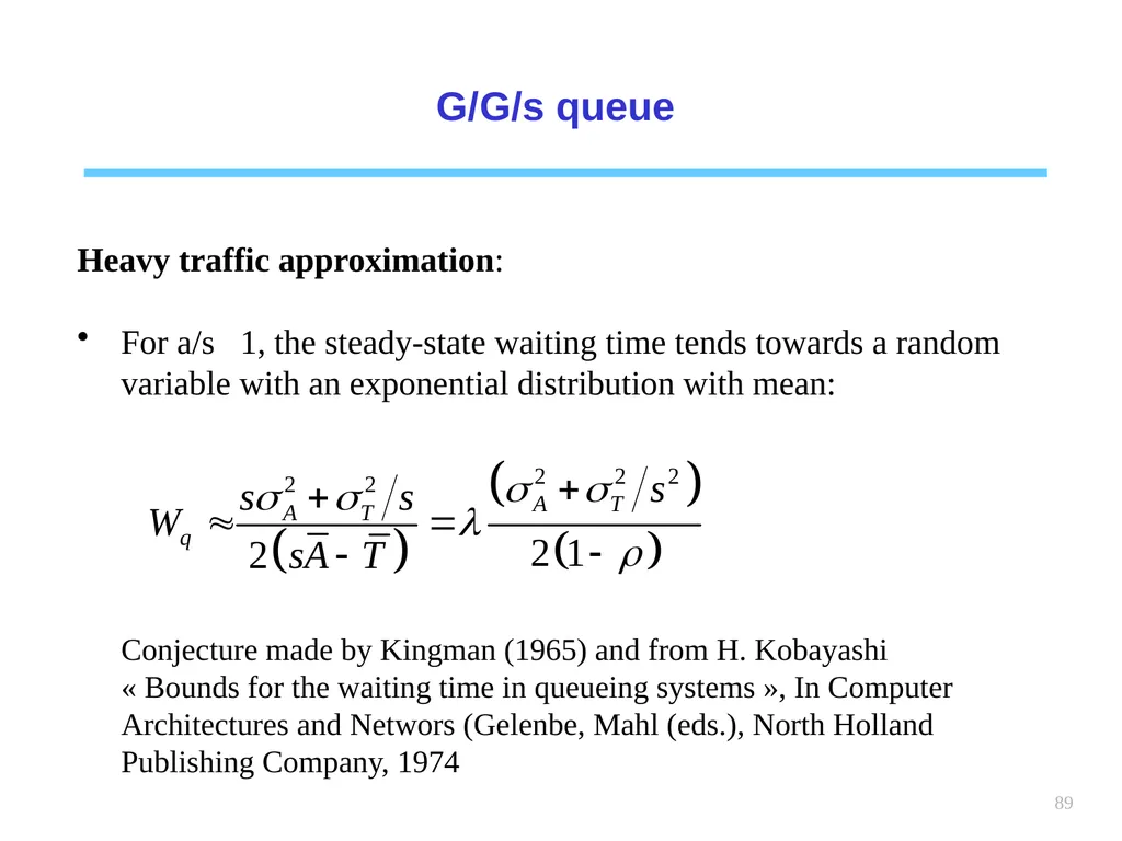
slide89. 89 G/G/s queue Heavy traffic approximation:

For a/s  1, the steady-state waiting time tends towards a random variable with an exponential distribution with mean: Conjecture made by Kingman (1965) and from H. Kobayashi « Bounds for the waiting time in queueing systems », In Computer Architectures and Networs (Gelenbe, Mahl (eds.), North Holland Publishing Company, 1974<br>
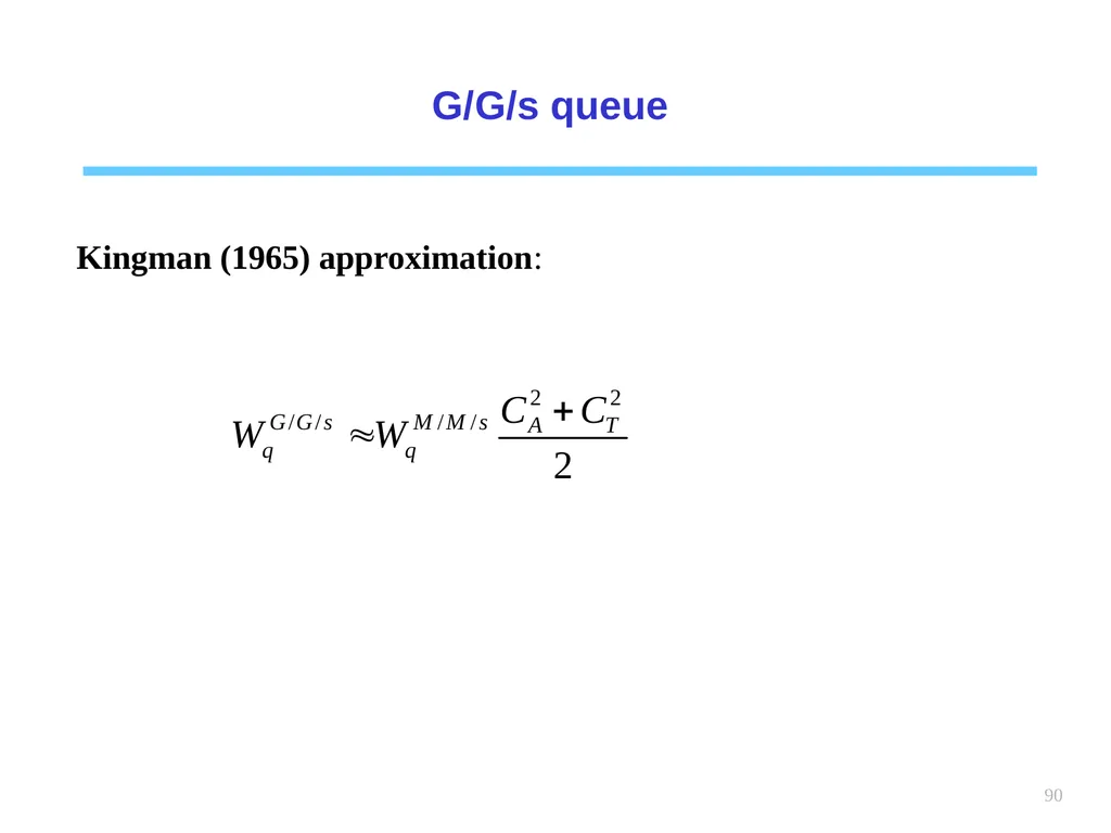
slide90. 90 G/G/s queue Kingman (1965) approximation:<br>