20250724 slides Dump Data yyyy/mm/dd title 1/N
Description: 20250724 slides Dump Data yyyymmdd title 1N Purity Systematics yyyymmdd title 2N Xsection - statisticErr Weighted average of Vincents purity and Catarinas purity Systematics of purity size of difference of two method 0.5
Related Topics
Download Presentation
"20250724 slides Dump Data yyyy/mm/dd title 1/N" is the property of its rightful owner. Permission is granted to download and print the materials on this website for personal, non-commercial use only, and to display it on your personal computer provided you do not modify the materials and that you retain all copyright notices contained in the materials. By downloading content from our website, you accept the terms of this agreement.
Presentation Transcript
slide1. 20250724 slides Dump Data yyyy/mm/dd title 1/N<br>
slide2. Purity Systematics yyyy/mm/dd title 2/N Xsection +/- statisticErr = Weighted average of Vincent’s purity and Catarina’s purity
Systematics of purity = size of difference of two method * 0.5 Example : W target / LL trigger<br>
slide3. Acceptance Systematics yyyy/mm/dd title 3/N Source#1 : statistical uncertainty of acceptance
Source#2 : Uncertainty of trigger efficiency and detector efficiency
Vincent’s study shows that the size of Source#2 is twice of Source#1. Example : W target / LL trigger Source#1 Source#2<br>
slide4. Acceptance Systematics yyyy/mm/dd title 4/N Systematic of acceptance of Source#1 can be easily obtained.
The total size of acceptance systematic is three times of source#1. Example : W target / LL trigger<br>
slide5. Slides of 20251003, 20251117 Study BLUE yyyy/mm/dd title 5/N<br>
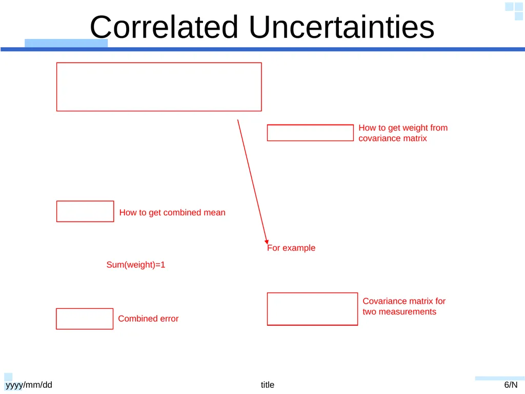
slide6. Correlated Uncertainties yyyy/mm/dd title 6/N Covariance matrix for two measurements How to get combined mean Sum(weight)=1 Combined error For example How to get weight from covariance matrix<br>
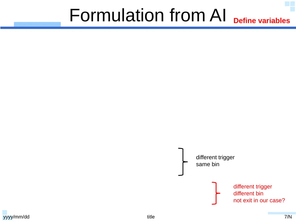
slide7. Formulation from AI yyyy/mm/dd title 7/N different trigger same bin different trigger different bin
not exit in our case? Define variables<br>
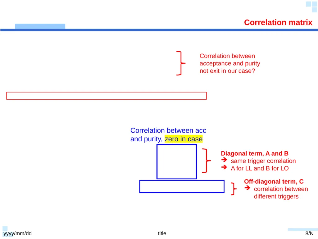
slide8. yyyy/mm/dd title 8/N Diagonal term, A and B
same trigger correlation
A for LL and B for LO Off-diagonal term, C
correlation between different triggers Correlation between acceptance and purity
not exit in our case? Correlation matrix Correlation between acc and purity, zero in case<br>
slide9. yyyy/mm/dd title 9/N Combined mean and sigma 0<rho<1 in our case<br>
slide10. yyyy/mm/dd title 10/N Example<br>
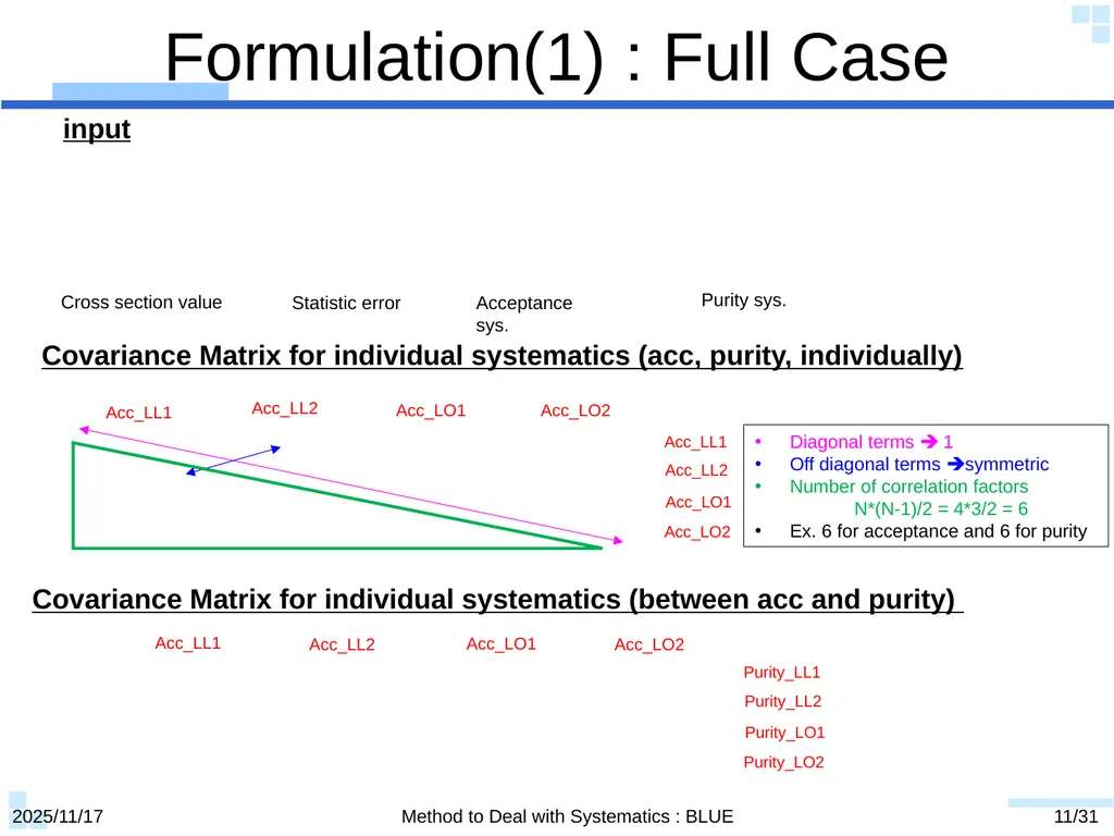
slide11. Formulation(1) : Full Case 2025/11/17 Method to Deal with Systematics : BLUE Cross section value Statistic error Acceptance sys. Purity sys. input Covariance Matrix for individual systematics (acc, purity, individually) Diagonal terms 1
Off diagonal terms symmetric
Number of correlation factors
N*(N-1)/2 = 4*3/2 = 6
Ex. 6 for acceptance and 6 for purity Covariance Matrix for individual systematics (between acc and purity) 11/31<br>
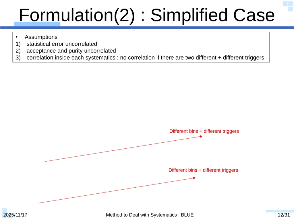
slide12. Formulation(2) : Simplified Case 2025/11/17 Method to Deal with Systematics : BLUE Assumptions
statistical error uncorrelated
acceptance and purity uncorrelated
correlation inside each systematics : no correlation if there are two different + different triggers Different bins + different triggers Different bins + different triggers 12/31<br>
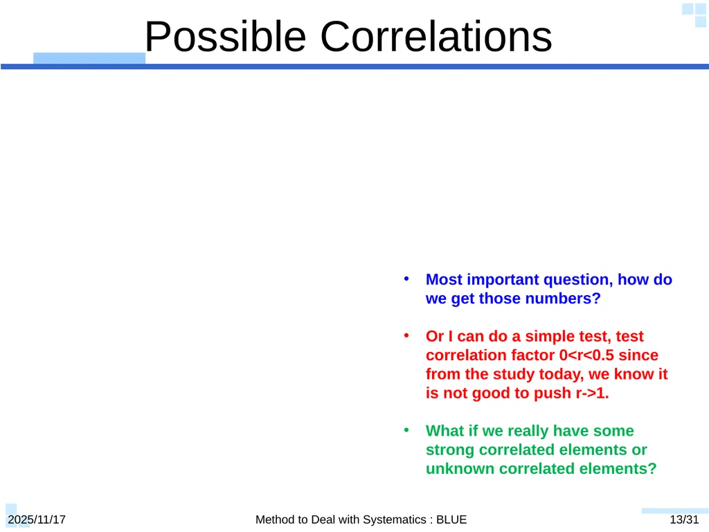
slide13. Possible Correlations 2025/11/17 Method to Deal with Systematics : BLUE Most important question, how do we get those numbers?
Or I can do a simple test, test correlation factor 0<r<0.5 since from the study today, we know it is not good to push r->1.
What if we really have some strong correlated elements or unknown correlated elements? 13/31<br>
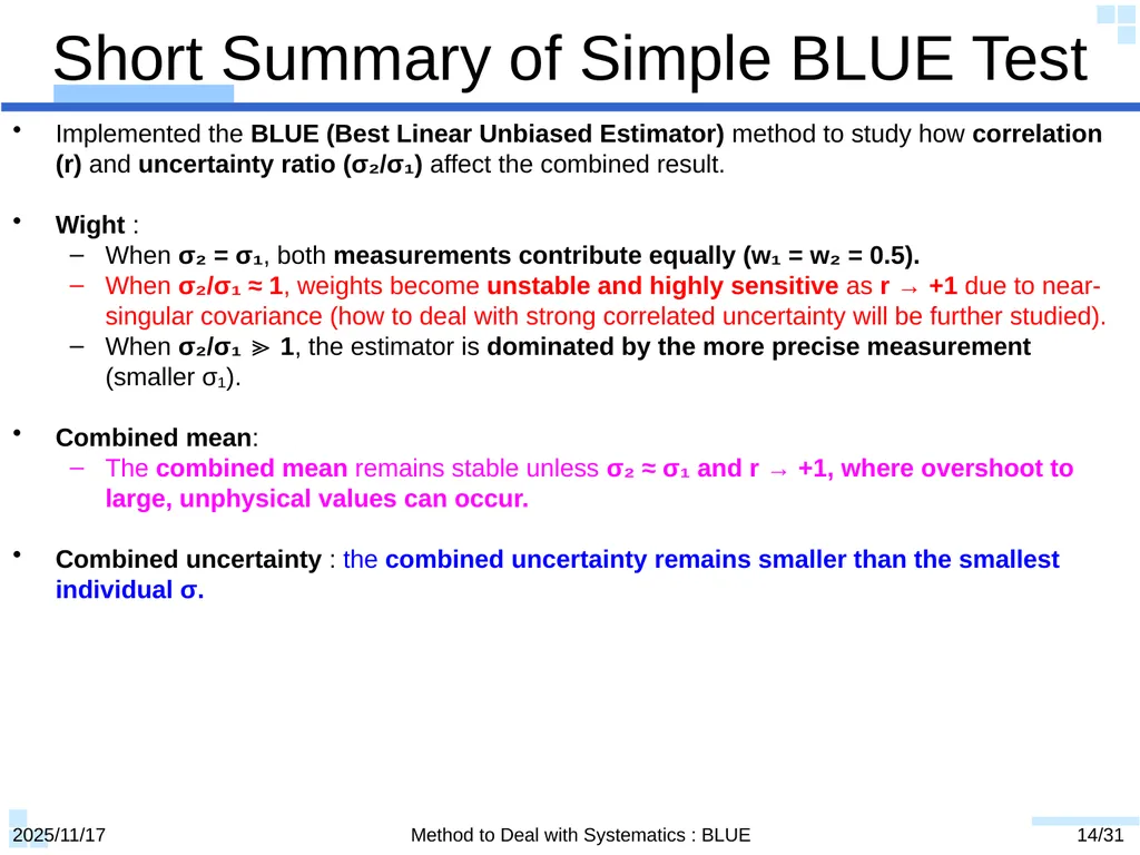
slide14. Short Summary of Simple BLUE Test 2025/11/17 Method to Deal with Systematics : BLUE Implemented the BLUE (Best Linear Unbiased Estimator) method to study how correlation (r) and uncertainty ratio (σ₂/σ₁) affect the combined result.
Wight :
When σ₂ = σ₁, both measurements contribute equally (w₁ = w₂ = 0.5).
When σ₂/σ₁ ≈ 1, weights become unstable and highly sensitive as r → +1 due to near-singular covariance (how to deal with strong correlated uncertainty will be further studied).
When σ₂/σ₁ ≫ 1, the estimator is dominated by the more precise measurement (smaller σ₁).
Combined mean:
The combined mean remains stable unless σ₂ ≈ σ₁ and r → +1, where overshoot to large, unphysical values can occur.
Combined uncertainty : the combined uncertainty remains smaller than the smallest individual σ. 14/31<br>
slide15. err_cy_txtFile_allCorr4.py BLUECombine yyyy/mm/dd title 15/N<br>
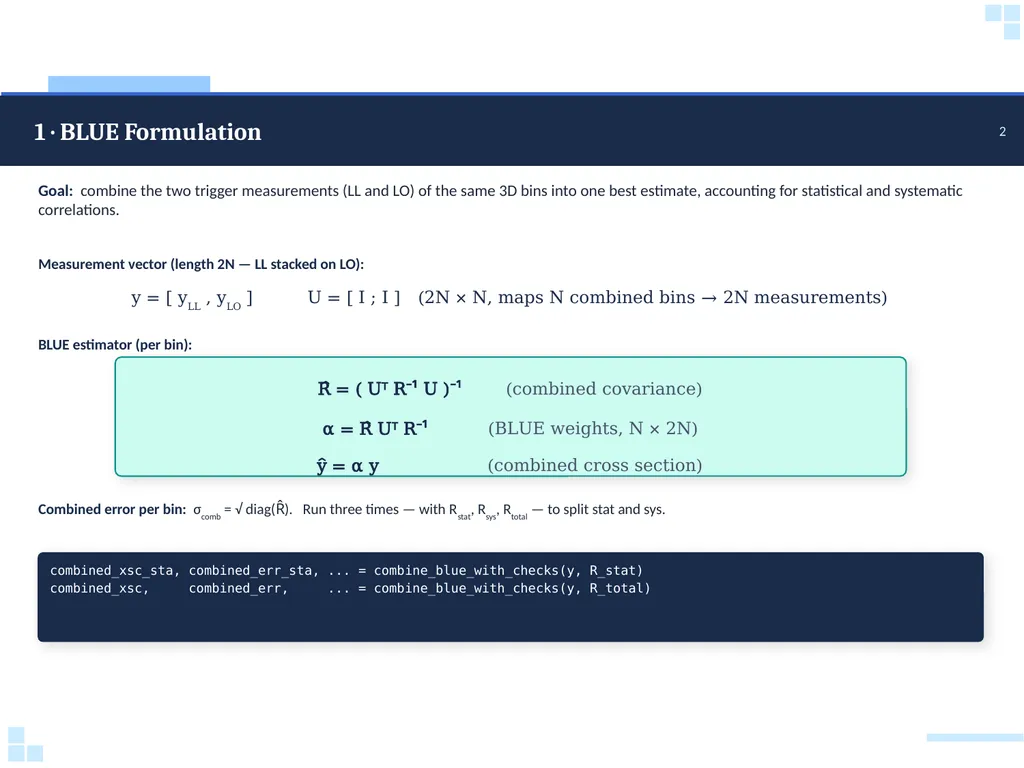
slide16. 1 · BLUE Formulation 2 Goal: combine the two trigger measurements (LL and LO) of the same 3D bins into one best estimate, accounting for statistical and systematic correlations. Measurement vector (length 2N — LL stacked on LO): y = [ yLL , yLO ] U = [ I ; I ] (2N × N, maps N combined bins → 2N measurements) BLUE estimator (per bin): R̂ = ( Uᵀ R⁻¹ U )⁻¹ (combined covariance) α = R̂ Uᵀ R⁻¹ (BLUE weights, N × 2N) ŷ = α y (combined cross section) Combined error per bin: σcomb = √ diag(R̂). Run three times — with Rstat, Rsys, Rtotal — to split stat and sys. combined_xsc_sta, combined_err_sta, ... = combine_blue_with_checks(y, R_stat)
combined_xsc, combined_err, ... = combine_blue_with_checks(y, R_total)<br>
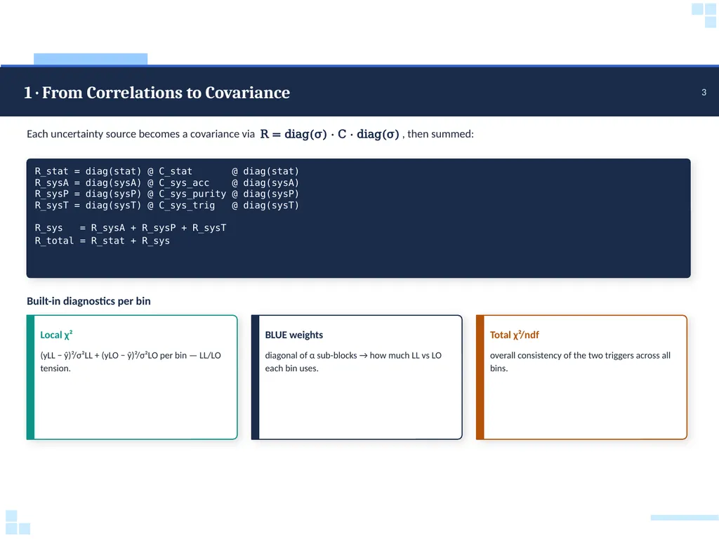
slide17. 1 · From Correlations to Covariance 3 Each uncertainty source becomes a covariance via R = diag(σ) · C · diag(σ) , then summed: R_stat = diag(stat) @ C_stat @ diag(stat)
R_sysA = diag(sysA) @ C_sys_acc @ diag(sysA)
R_sysP = diag(sysP) @ C_sys_purity @ diag(sysP)
R_sysT = diag(sysT) @ C_sys_trig @ diag(sysT)
R_sys = R_sysA + R_sysP + R_sysT
R_total = R_stat + R_sys Built-in diagnostics per bin Local χ² (yLL − ŷ)²/σ²LL + (yLO − ŷ)²/σ²LO per bin — LL/LO tension. BLUE weights diagonal of α sub-blocks → how much LL vs LO each bin uses. Total χ²/ndf overall consistency of the two triggers across all bins.<br>
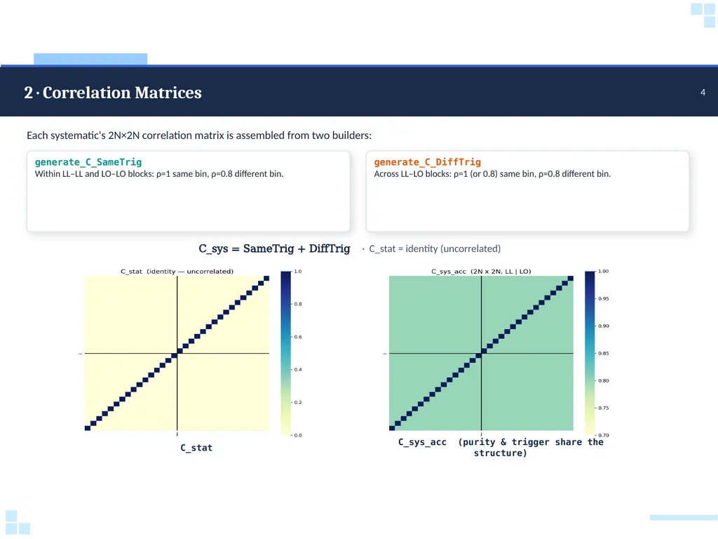
slide18. 2 · Correlation Matrices 4 Each systematic's 2N×2N correlation matrix is assembled from two builders: generate_C_SameTrig
Within LL–LL and LO–LO blocks: ρ=1 same bin, ρ=0.8 different bin. generate_C_DiffTrig
Across LL–LO blocks: ρ=1 (or 0.8) same bin, ρ=0.8 different bin. C_sys = SameTrig + DiffTrig · C_stat = identity (uncorrelated) C_stat C_sys_acc (purity & trigger share the structure)<br>
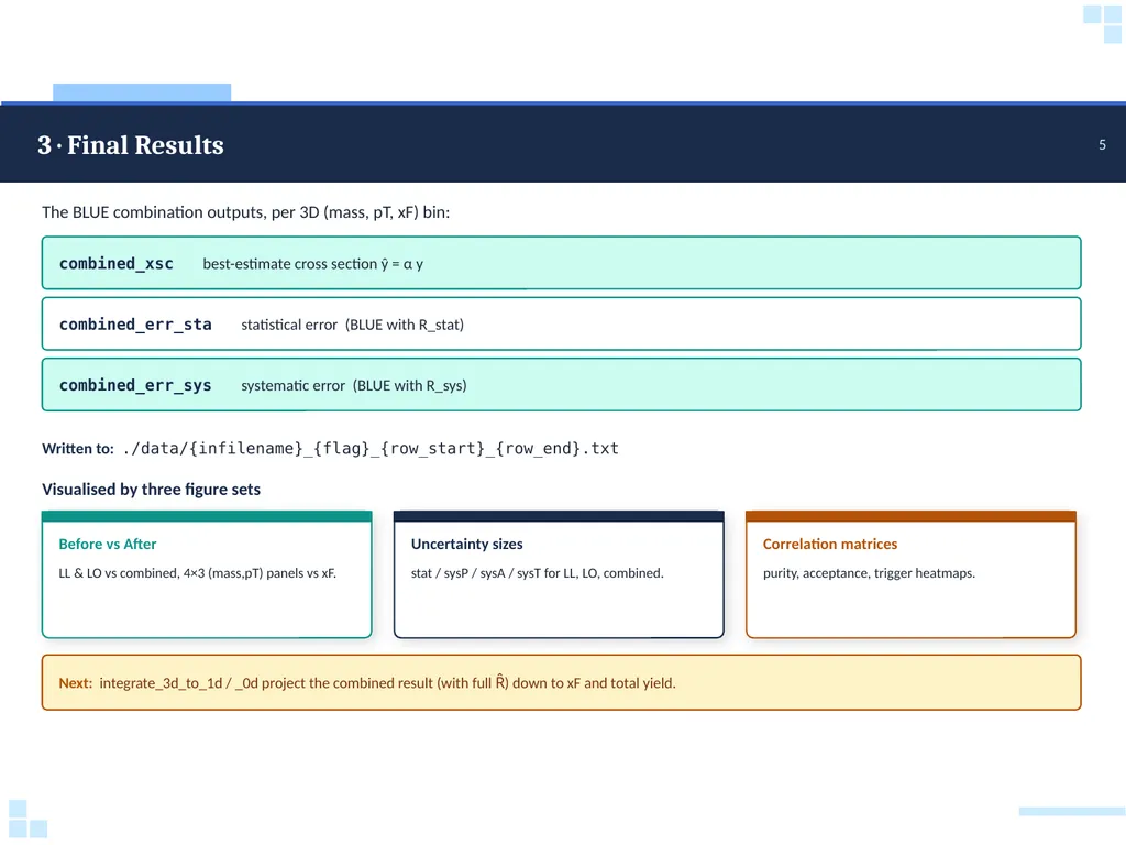
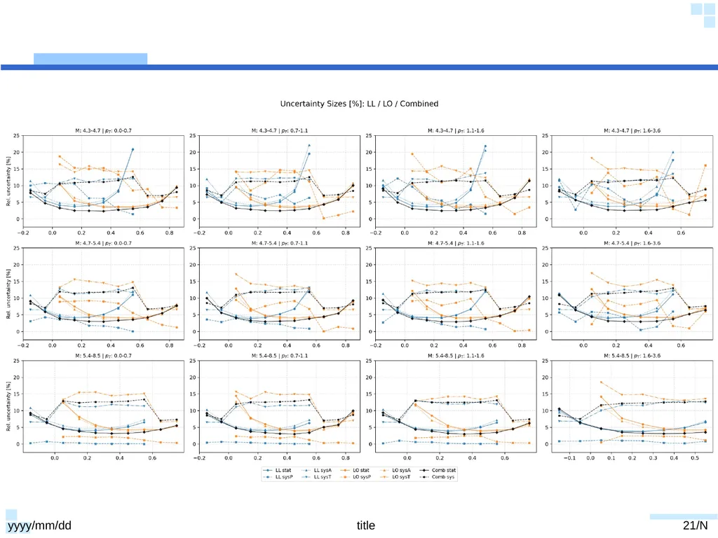
slide19. 3 · Final Results 5 The BLUE combination outputs, per 3D (mass, pT, xF) bin: combined_xsc best-estimate cross section ŷ = α y combined_err_sta statistical error (BLUE with R_stat) combined_err_sys systematic error (BLUE with R_sys) Written to: ./data/{infilename}_{flag}_{row_start}_{row_end}.txt Visualised by three figure sets Before vs After LL & LO vs combined, 4×3 (mass,pT) panels vs xF. Uncertainty sizes stat / sysP / sysA / sysT for LL, LO, combined. Correlation matrices purity, acceptance, trigger heatmaps. Next: integrate_3d_to_1d / _0d project the combined result (with full R̂) down to xF and total yield.<br>
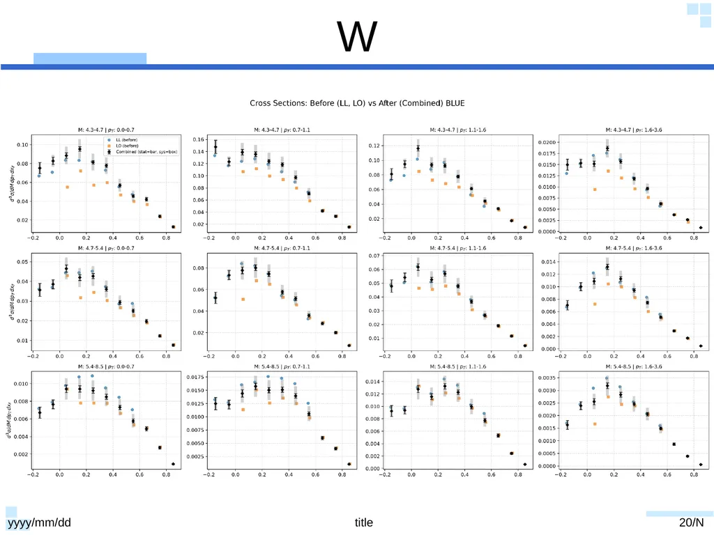
slide20. W yyyy/mm/dd title 20/N<br>
slide21. yyyy/mm/dd title 21/N<br>
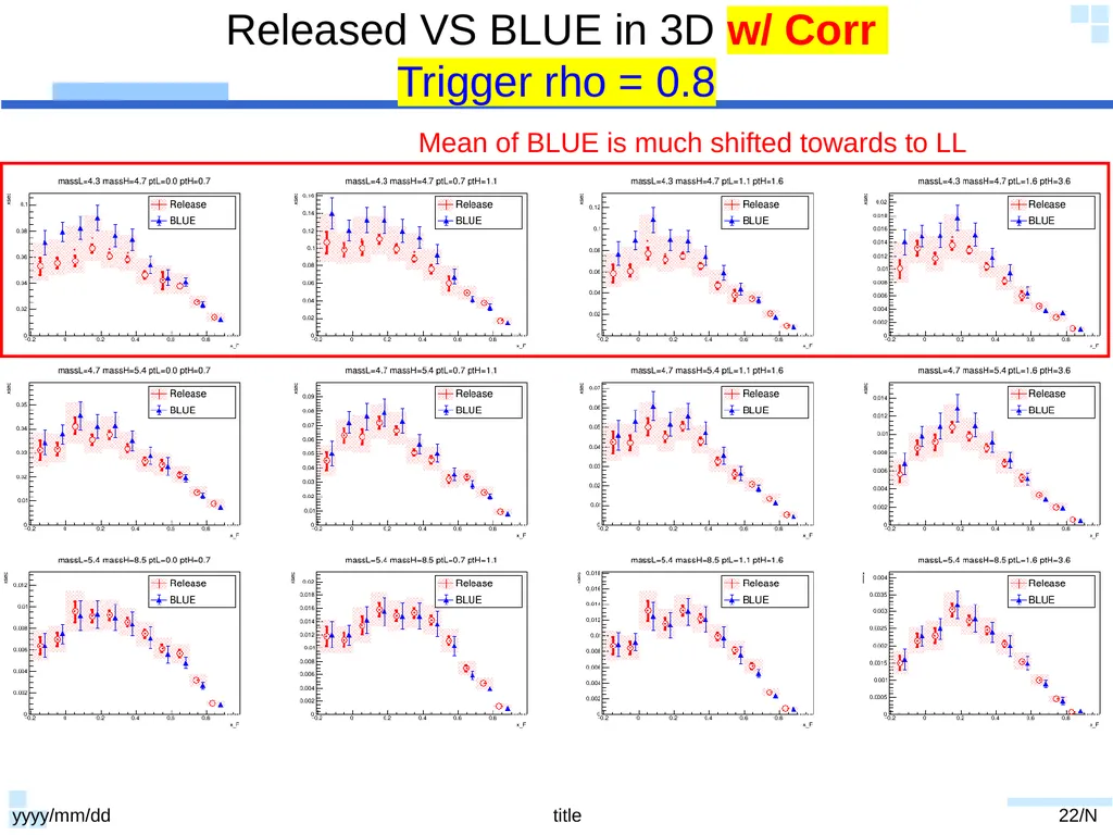
slide22. Released VS BLUE in 3D w/ Corr Trigger rho = 0.8 yyyy/mm/dd title 22/N Mean of BLUE is much shifted towards to LL<br>
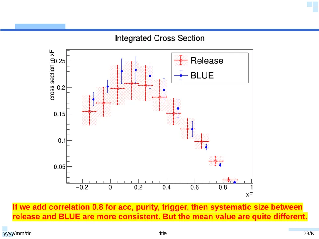
slide23. yyyy/mm/dd title 23/N If we add correlation 0.8 for acc, purity, trigger, then systematic size between release and BLUE are more consistent. But the mean value are quite different.<br>
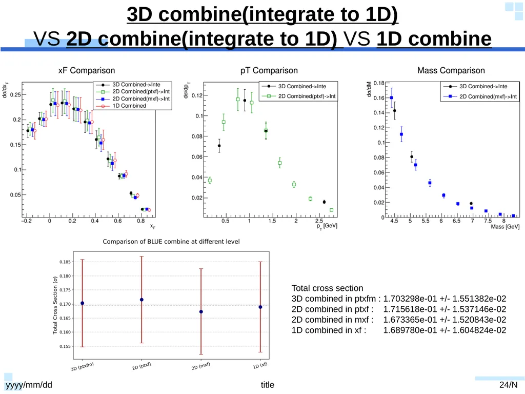
slide24. 3D combine(integrate to 1D)VS 2D combine(integrate to 1D) VS 1D combine yyyy/mm/dd title 24/N W Total cross section
3D combined in ptxfm : 1.703298e-01 +/- 1.551382e-02
2D combined in ptxf : 1.715618e-01 +/- 1.537146e-02
2D combined in mxf : 1.673365e-01 +/- 1.520843e-02
1D combined in xf : 1.689780e-01 +/- 1.604824e-02<br>
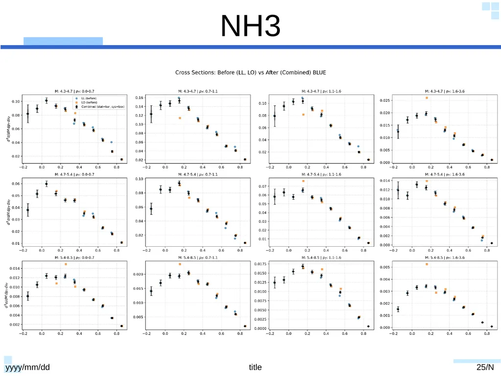
slide25. NH3 yyyy/mm/dd title 25/N<br>
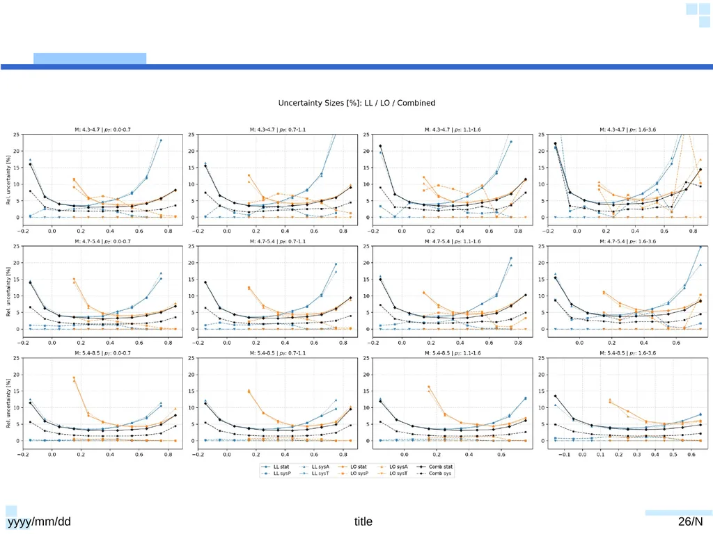
slide26. yyyy/mm/dd title 26/N<br>
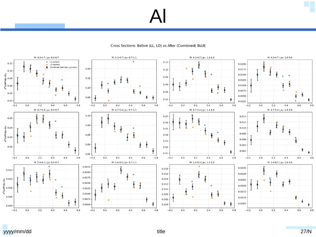
slide27. Al yyyy/mm/dd title 27/N<br>
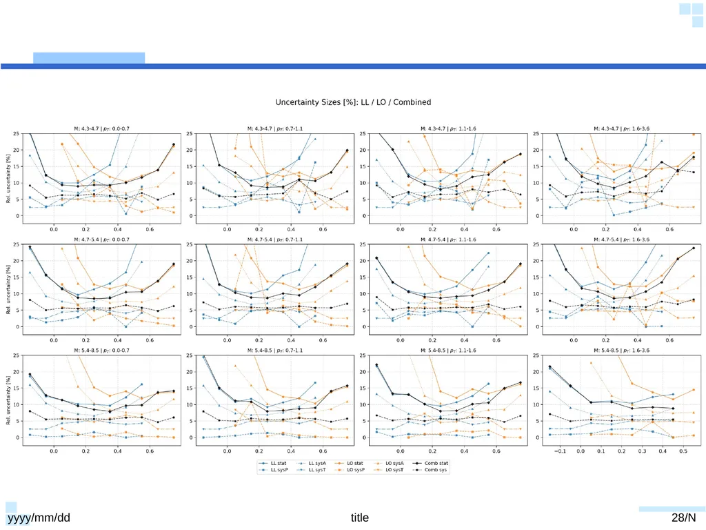
slide28. yyyy/mm/dd title 28/N<br>
slide29. More realistic sys and corr yyyy/mm/dd title 29/N https://docs.google.com/document/d/1RANY0-G8v7JsBg6vcyVTTX0N6OD3O04ShqOp34YLw5w/edit?tab=t.0<br>
slide30. Acc Sys yyyy/mm/dd title 30/N<br>
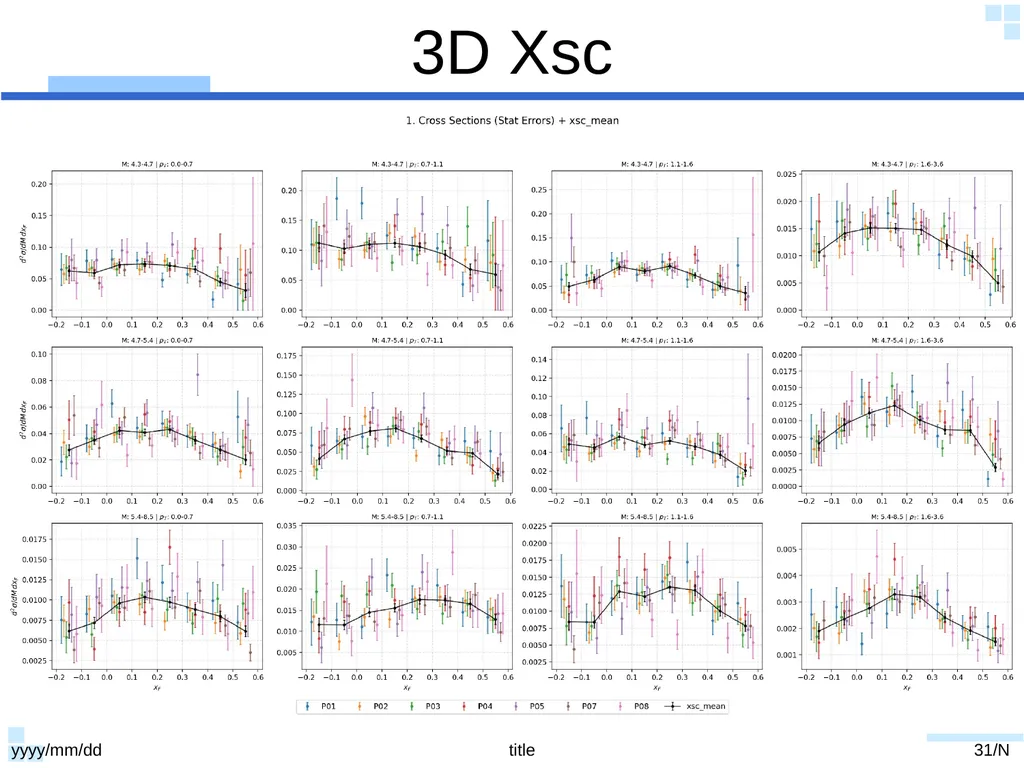
slide31. 3D Xsc yyyy/mm/dd title 31/N<br>
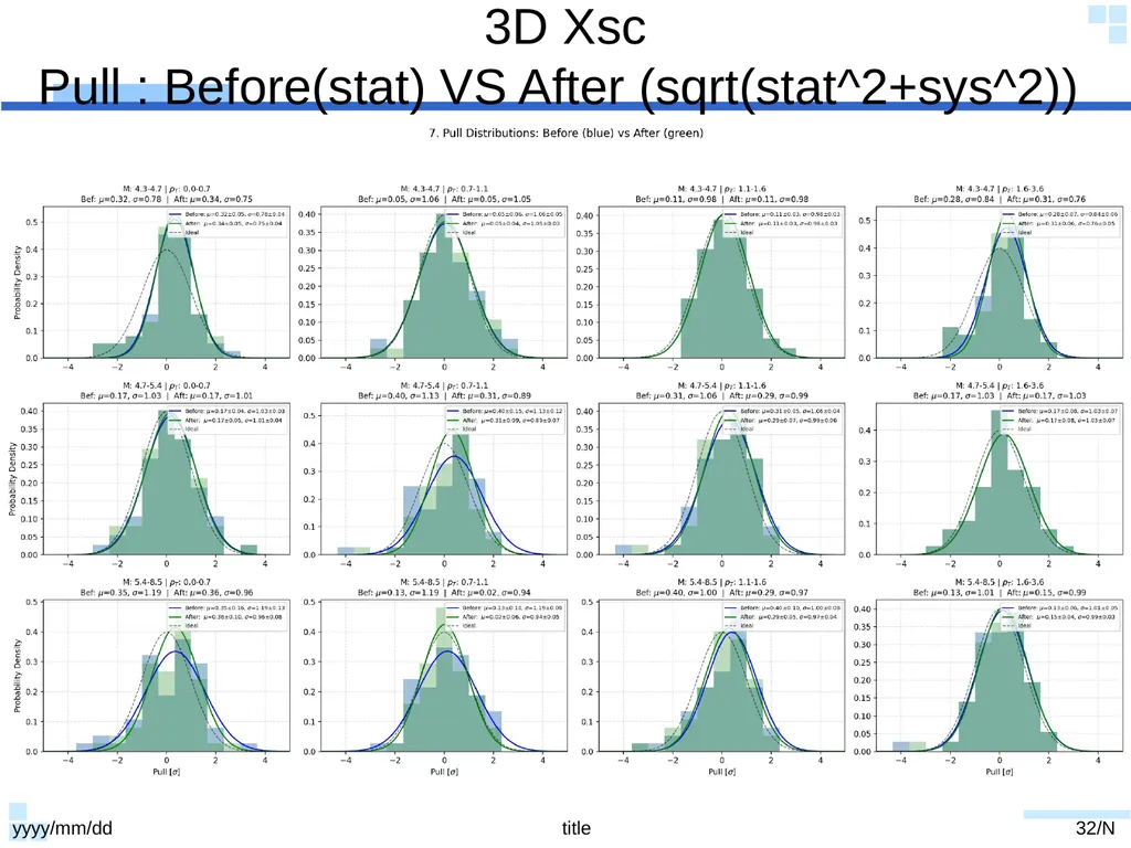
slide32. 3D XscPull : Before(stat) VS After (sqrt(stat^2+sys^2)) yyyy/mm/dd title 32/N<br>
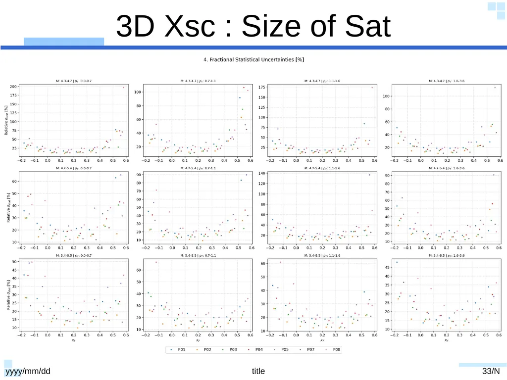
slide33. 3D Xsc : Size of Sat yyyy/mm/dd title 33/N<br>
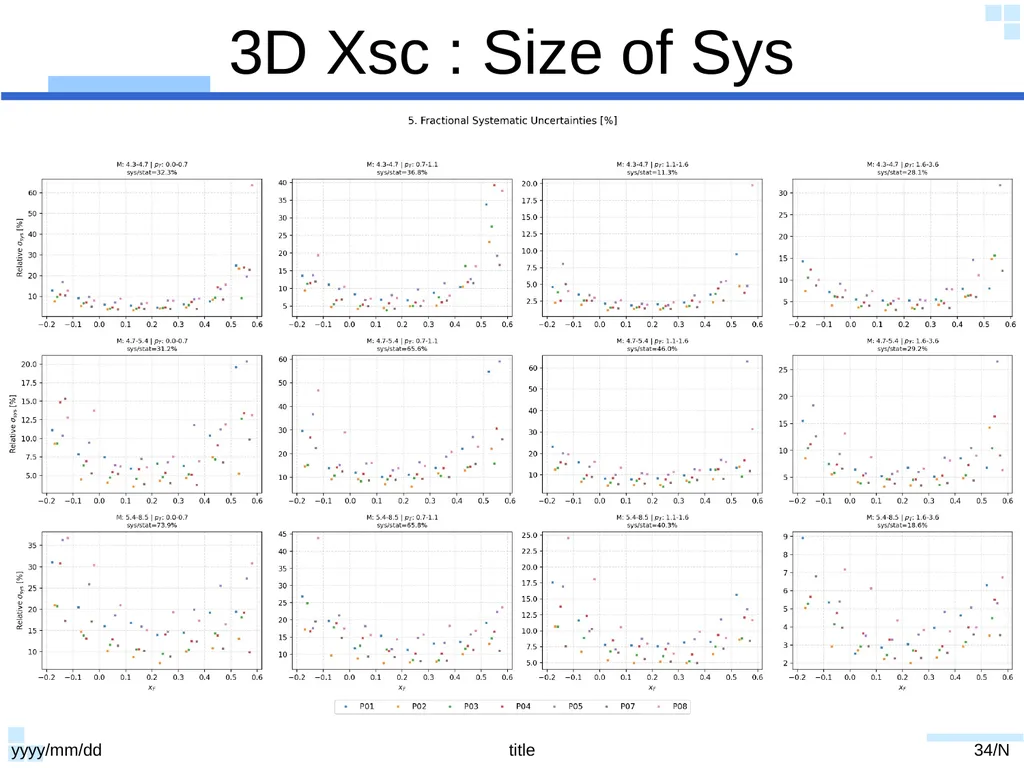
slide34. 3D Xsc : Size of Sys yyyy/mm/dd title 34/N<br>
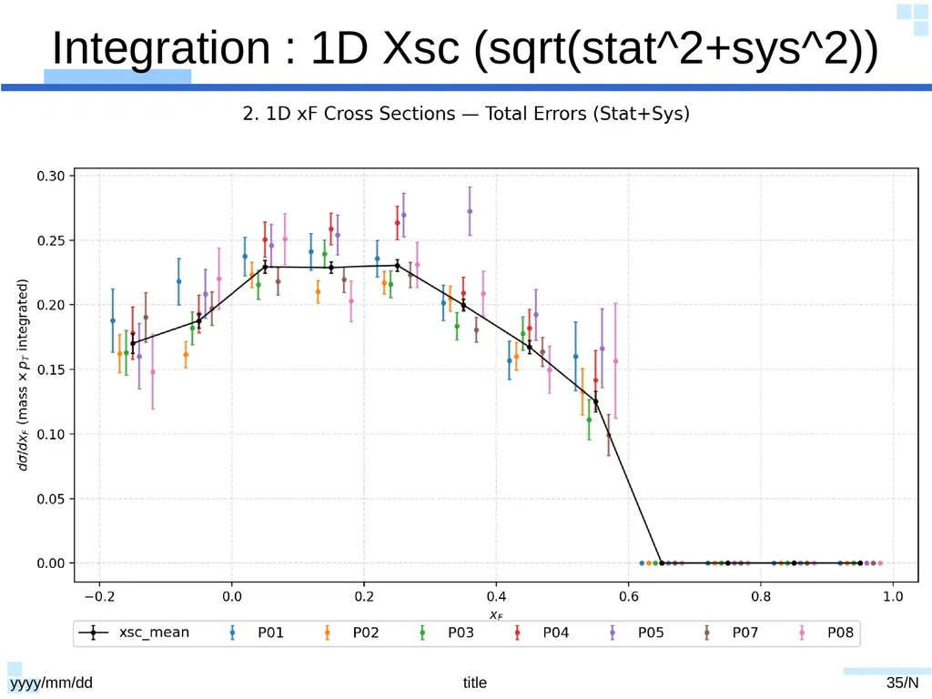
slide35. Integration : 1D Xsc (sqrt(stat^2+sys^2)) yyyy/mm/dd title 35/N<br>
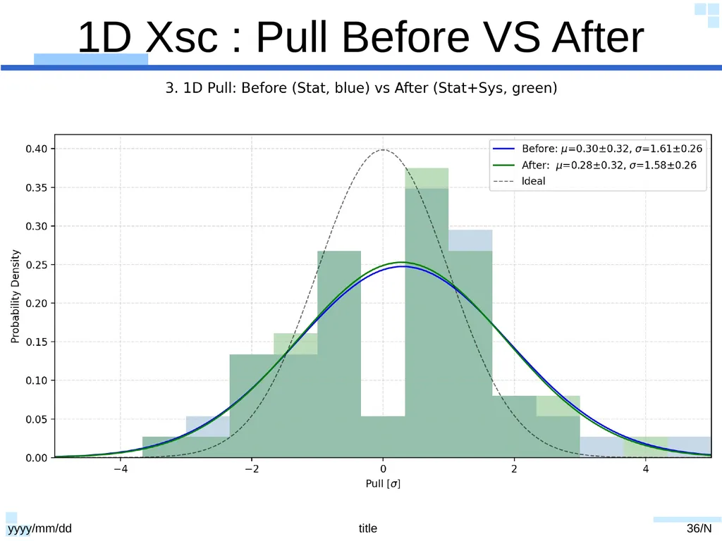
slide36. 1D Xsc : Pull Before VS After yyyy/mm/dd title 36/N<br>
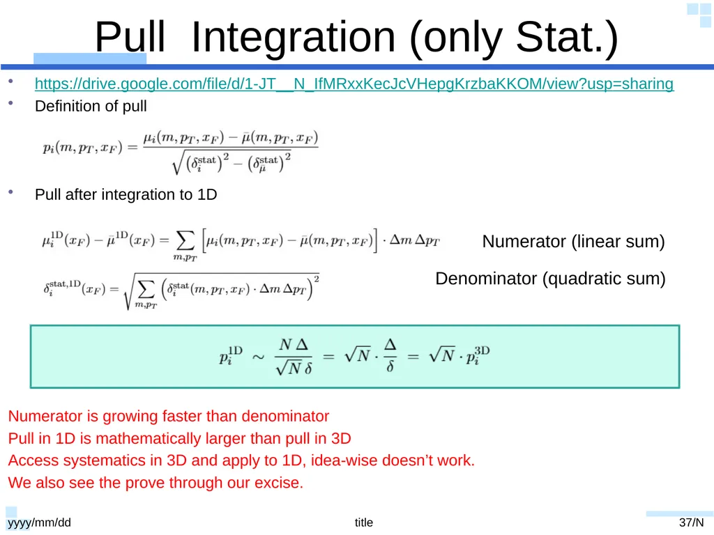
slide37. Pull Integration (only Stat.) yyyy/mm/dd title 37/N https://drive.google.com/file/d/1-JT__N_IfMRxxKecJcVHepgKrzbaKKOM/view?usp=sharing
Definition of pull
Pull after integration to 1D
Numerator is growing faster than denominator
Pull in 1D is mathematically larger than pull in 3D
Access systematics in 3D and apply to 1D, idea-wise doesn’t work.
We also see the prove through our excise. Numerator (linear sum) Denominator (quadratic sum)<br>
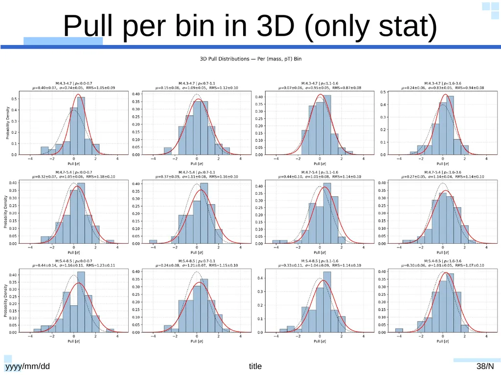
slide38. Pull per bin in 3D (only stat) yyyy/mm/dd title 38/N<br>
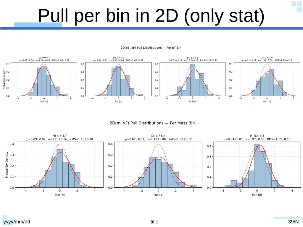
slide39. Pull per bin in 2D (only stat) yyyy/mm/dd title 39/N<br>
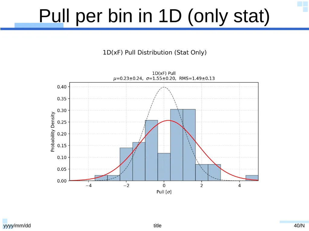
slide40. Pull per bin in 1D (only stat) yyyy/mm/dd title 40/N<br>
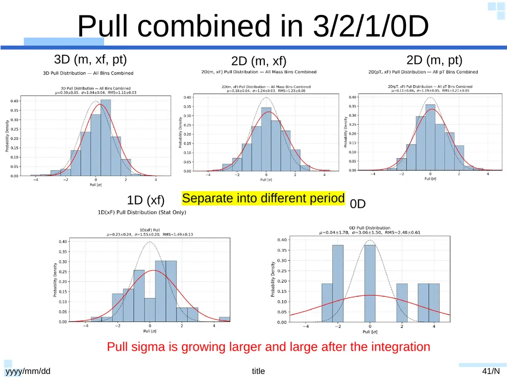
slide41. Pull combined in 3/2/1/0D yyyy/mm/dd title 41/N 3D (m, xf, pt) 2D (m, xf) 2D (m, pt) 1D (xf) 0D Pull sigma is growing larger and large after the integration Separate into different period<br>
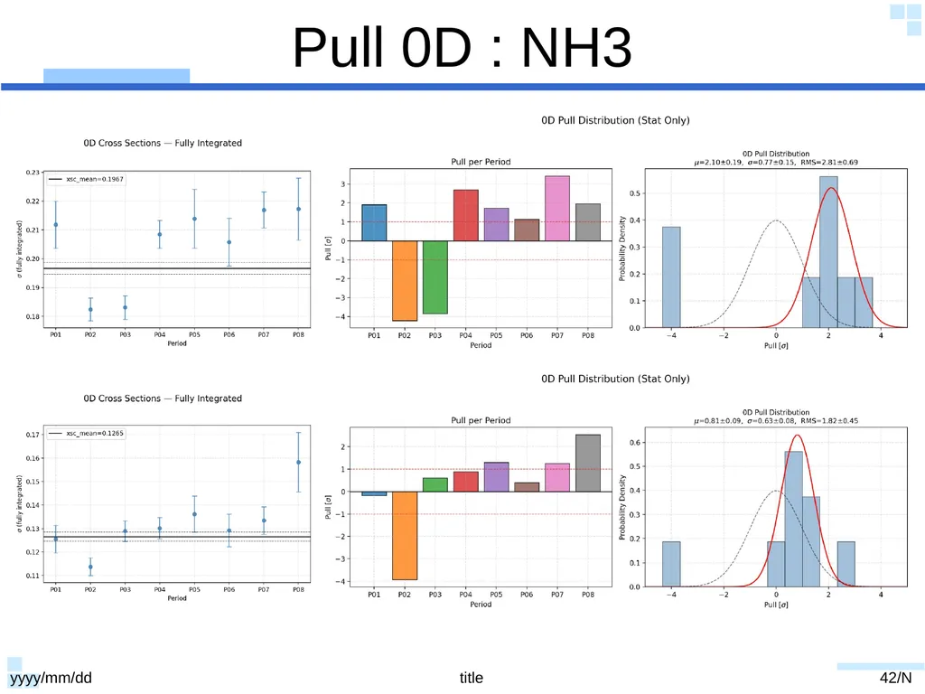
slide42. Pull 0D : NH3 yyyy/mm/dd title 42/N<br>
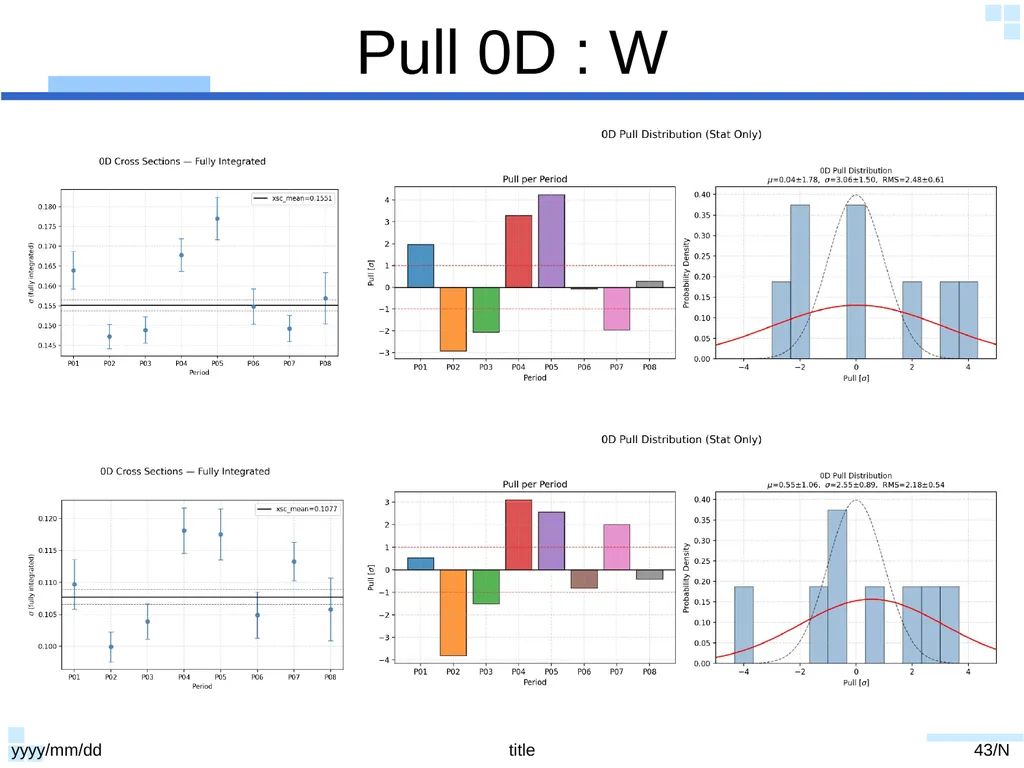
slide43. Pull 0D : W yyyy/mm/dd title 43/N<br>
slide2. Purity Systematics yyyy/mm/dd title 2/N Xsection +/- statisticErr = Weighted average of Vincent’s purity and Catarina’s purity
Systematics of purity = size of difference of two method * 0.5 Example : W target / LL trigger<br>
slide3. Acceptance Systematics yyyy/mm/dd title 3/N Source#1 : statistical uncertainty of acceptance
Source#2 : Uncertainty of trigger efficiency and detector efficiency
Vincent’s study shows that the size of Source#2 is twice of Source#1. Example : W target / LL trigger Source#1 Source#2<br>
slide4. Acceptance Systematics yyyy/mm/dd title 4/N Systematic of acceptance of Source#1 can be easily obtained.
The total size of acceptance systematic is three times of source#1. Example : W target / LL trigger<br>
slide5. Slides of 20251003, 20251117 Study BLUE yyyy/mm/dd title 5/N<br>
slide6. Correlated Uncertainties yyyy/mm/dd title 6/N Covariance matrix for two measurements How to get combined mean Sum(weight)=1 Combined error For example How to get weight from covariance matrix<br>
slide7. Formulation from AI yyyy/mm/dd title 7/N different trigger same bin different trigger different bin
not exit in our case? Define variables<br>
slide8. yyyy/mm/dd title 8/N Diagonal term, A and B
same trigger correlation
A for LL and B for LO Off-diagonal term, C
correlation between different triggers Correlation between acceptance and purity
not exit in our case? Correlation matrix Correlation between acc and purity, zero in case<br>
slide9. yyyy/mm/dd title 9/N Combined mean and sigma 0<rho<1 in our case<br>
slide10. yyyy/mm/dd title 10/N Example<br>
slide11. Formulation(1) : Full Case 2025/11/17 Method to Deal with Systematics : BLUE Cross section value Statistic error Acceptance sys. Purity sys. input Covariance Matrix for individual systematics (acc, purity, individually) Diagonal terms 1
Off diagonal terms symmetric
Number of correlation factors
N*(N-1)/2 = 4*3/2 = 6
Ex. 6 for acceptance and 6 for purity Covariance Matrix for individual systematics (between acc and purity) 11/31<br>
slide12. Formulation(2) : Simplified Case 2025/11/17 Method to Deal with Systematics : BLUE Assumptions
statistical error uncorrelated
acceptance and purity uncorrelated
correlation inside each systematics : no correlation if there are two different + different triggers Different bins + different triggers Different bins + different triggers 12/31<br>
slide13. Possible Correlations 2025/11/17 Method to Deal with Systematics : BLUE Most important question, how do we get those numbers?
Or I can do a simple test, test correlation factor 0<r<0.5 since from the study today, we know it is not good to push r->1.
What if we really have some strong correlated elements or unknown correlated elements? 13/31<br>
slide14. Short Summary of Simple BLUE Test 2025/11/17 Method to Deal with Systematics : BLUE Implemented the BLUE (Best Linear Unbiased Estimator) method to study how correlation (r) and uncertainty ratio (σ₂/σ₁) affect the combined result.
Wight :
When σ₂ = σ₁, both measurements contribute equally (w₁ = w₂ = 0.5).
When σ₂/σ₁ ≈ 1, weights become unstable and highly sensitive as r → +1 due to near-singular covariance (how to deal with strong correlated uncertainty will be further studied).
When σ₂/σ₁ ≫ 1, the estimator is dominated by the more precise measurement (smaller σ₁).
Combined mean:
The combined mean remains stable unless σ₂ ≈ σ₁ and r → +1, where overshoot to large, unphysical values can occur.
Combined uncertainty : the combined uncertainty remains smaller than the smallest individual σ. 14/31<br>
slide15. err_cy_txtFile_allCorr4.py BLUECombine yyyy/mm/dd title 15/N<br>
slide16. 1 · BLUE Formulation 2 Goal: combine the two trigger measurements (LL and LO) of the same 3D bins into one best estimate, accounting for statistical and systematic correlations. Measurement vector (length 2N — LL stacked on LO): y = [ yLL , yLO ] U = [ I ; I ] (2N × N, maps N combined bins → 2N measurements) BLUE estimator (per bin): R̂ = ( Uᵀ R⁻¹ U )⁻¹ (combined covariance) α = R̂ Uᵀ R⁻¹ (BLUE weights, N × 2N) ŷ = α y (combined cross section) Combined error per bin: σcomb = √ diag(R̂). Run three times — with Rstat, Rsys, Rtotal — to split stat and sys. combined_xsc_sta, combined_err_sta, ... = combine_blue_with_checks(y, R_stat)
combined_xsc, combined_err, ... = combine_blue_with_checks(y, R_total)<br>
slide17. 1 · From Correlations to Covariance 3 Each uncertainty source becomes a covariance via R = diag(σ) · C · diag(σ) , then summed: R_stat = diag(stat) @ C_stat @ diag(stat)
R_sysA = diag(sysA) @ C_sys_acc @ diag(sysA)
R_sysP = diag(sysP) @ C_sys_purity @ diag(sysP)
R_sysT = diag(sysT) @ C_sys_trig @ diag(sysT)
R_sys = R_sysA + R_sysP + R_sysT
R_total = R_stat + R_sys Built-in diagnostics per bin Local χ² (yLL − ŷ)²/σ²LL + (yLO − ŷ)²/σ²LO per bin — LL/LO tension. BLUE weights diagonal of α sub-blocks → how much LL vs LO each bin uses. Total χ²/ndf overall consistency of the two triggers across all bins.<br>
slide18. 2 · Correlation Matrices 4 Each systematic's 2N×2N correlation matrix is assembled from two builders: generate_C_SameTrig
Within LL–LL and LO–LO blocks: ρ=1 same bin, ρ=0.8 different bin. generate_C_DiffTrig
Across LL–LO blocks: ρ=1 (or 0.8) same bin, ρ=0.8 different bin. C_sys = SameTrig + DiffTrig · C_stat = identity (uncorrelated) C_stat C_sys_acc (purity & trigger share the structure)<br>
slide19. 3 · Final Results 5 The BLUE combination outputs, per 3D (mass, pT, xF) bin: combined_xsc best-estimate cross section ŷ = α y combined_err_sta statistical error (BLUE with R_stat) combined_err_sys systematic error (BLUE with R_sys) Written to: ./data/{infilename}_{flag}_{row_start}_{row_end}.txt Visualised by three figure sets Before vs After LL & LO vs combined, 4×3 (mass,pT) panels vs xF. Uncertainty sizes stat / sysP / sysA / sysT for LL, LO, combined. Correlation matrices purity, acceptance, trigger heatmaps. Next: integrate_3d_to_1d / _0d project the combined result (with full R̂) down to xF and total yield.<br>
slide20. W yyyy/mm/dd title 20/N<br>
slide21. yyyy/mm/dd title 21/N<br>
slide22. Released VS BLUE in 3D w/ Corr Trigger rho = 0.8 yyyy/mm/dd title 22/N Mean of BLUE is much shifted towards to LL<br>
slide23. yyyy/mm/dd title 23/N If we add correlation 0.8 for acc, purity, trigger, then systematic size between release and BLUE are more consistent. But the mean value are quite different.<br>
slide24. 3D combine(integrate to 1D)VS 2D combine(integrate to 1D) VS 1D combine yyyy/mm/dd title 24/N W Total cross section
3D combined in ptxfm : 1.703298e-01 +/- 1.551382e-02
2D combined in ptxf : 1.715618e-01 +/- 1.537146e-02
2D combined in mxf : 1.673365e-01 +/- 1.520843e-02
1D combined in xf : 1.689780e-01 +/- 1.604824e-02<br>
slide25. NH3 yyyy/mm/dd title 25/N<br>
slide26. yyyy/mm/dd title 26/N<br>
slide27. Al yyyy/mm/dd title 27/N<br>
slide28. yyyy/mm/dd title 28/N<br>
slide29. More realistic sys and corr yyyy/mm/dd title 29/N https://docs.google.com/document/d/1RANY0-G8v7JsBg6vcyVTTX0N6OD3O04ShqOp34YLw5w/edit?tab=t.0<br>
slide30. Acc Sys yyyy/mm/dd title 30/N<br>
slide31. 3D Xsc yyyy/mm/dd title 31/N<br>
slide32. 3D XscPull : Before(stat) VS After (sqrt(stat^2+sys^2)) yyyy/mm/dd title 32/N<br>
slide33. 3D Xsc : Size of Sat yyyy/mm/dd title 33/N<br>
slide34. 3D Xsc : Size of Sys yyyy/mm/dd title 34/N<br>
slide35. Integration : 1D Xsc (sqrt(stat^2+sys^2)) yyyy/mm/dd title 35/N<br>
slide36. 1D Xsc : Pull Before VS After yyyy/mm/dd title 36/N<br>
slide37. Pull Integration (only Stat.) yyyy/mm/dd title 37/N https://drive.google.com/file/d/1-JT__N_IfMRxxKecJcVHepgKrzbaKKOM/view?usp=sharing
Definition of pull
Pull after integration to 1D
Numerator is growing faster than denominator
Pull in 1D is mathematically larger than pull in 3D
Access systematics in 3D and apply to 1D, idea-wise doesn’t work.
We also see the prove through our excise. Numerator (linear sum) Denominator (quadratic sum)<br>
slide38. Pull per bin in 3D (only stat) yyyy/mm/dd title 38/N<br>
slide39. Pull per bin in 2D (only stat) yyyy/mm/dd title 39/N<br>
slide40. Pull per bin in 1D (only stat) yyyy/mm/dd title 40/N<br>
slide41. Pull combined in 3/2/1/0D yyyy/mm/dd title 41/N 3D (m, xf, pt) 2D (m, xf) 2D (m, pt) 1D (xf) 0D Pull sigma is growing larger and large after the integration Separate into different period<br>
slide42. Pull 0D : NH3 yyyy/mm/dd title 42/N<br>
slide43. Pull 0D : W yyyy/mm/dd title 43/N<br>