Adapted from a presentation by Richard Allen, 2011
Description: Adapted from a presentation by Richard Allen, 2011 Oct 2015 consultsupercomputingchallenge.org Supercomputing Around Us: Sensors and Data 1 Computational Science, Agent Based and Mathematical Modeling Computational Science? Computational
Related Topics
Download Presentation
"Adapted from a presentation by Richard Allen, 2011" is the property of its rightful owner. Permission is granted to download and print the materials on this website for personal, non-commercial use only, and to display it on your personal computer provided you do not modify the materials and that you retain all copyright notices contained in the materials. By downloading content from our website, you accept the terms of this agreement.
Presentation Transcript
slide1. Adapted from a presentation by Richard Allen, 2011 Oct 2015 © consult@supercomputingchallenge.org Supercomputing Around Us: Sensors and Data 1 Computational Science,Agent Based and Mathematical Modeling<br>
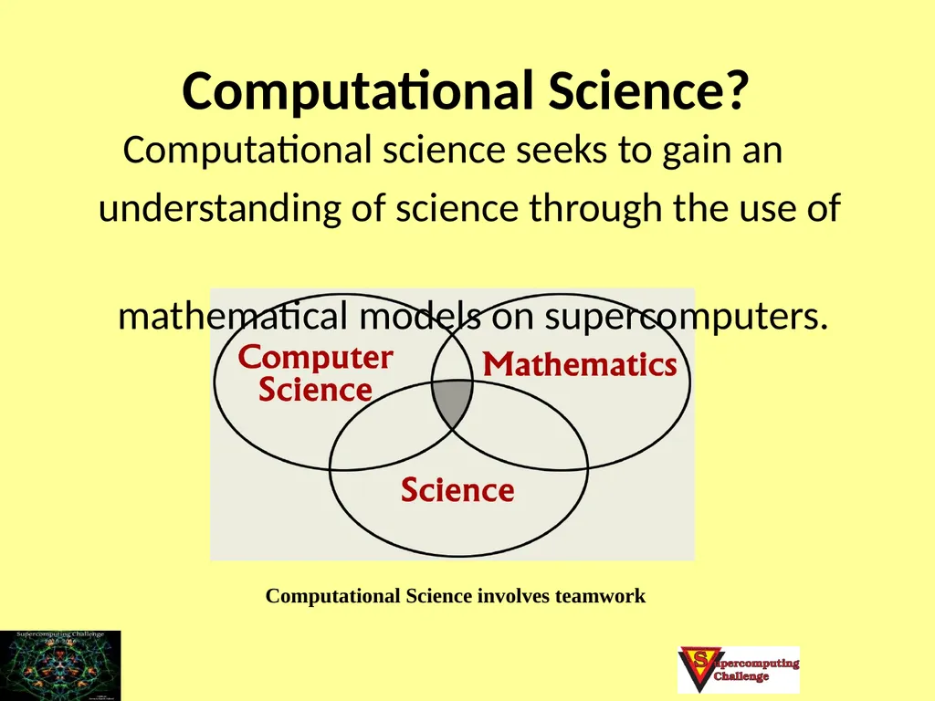
slide2. Computational Science? Computational science seeks to gain an
understanding of science through the use of
mathematical models on supercomputers. Computational Science involves teamwork<br>
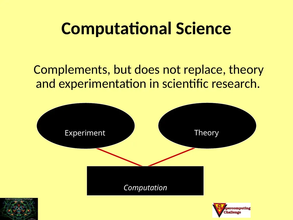
slide3. Computational Science Complements, but does not replace, theory and experimentation in scientific research.<br>
slide4. Computational Science Is often used in place of experiments when experiments are too large, too expensive, too dangerous, or too time consuming.
Can be useful in “what if” studies; e.g. to investigate the use of pathogens (viruses, bacteria, fungi) to control an insect population.
Is a modern tool for scientific investigation.<br>
slide5. Computational Science Has emerged as a powerful, indispensable tool for studying a variety of problems in scientific research, product and process development, and manufacturing. Seismology
Climate modeling
Economics
Environment
Material research Drug design
Manufacturing
Medicine
Biology Analyze - Predict<br>
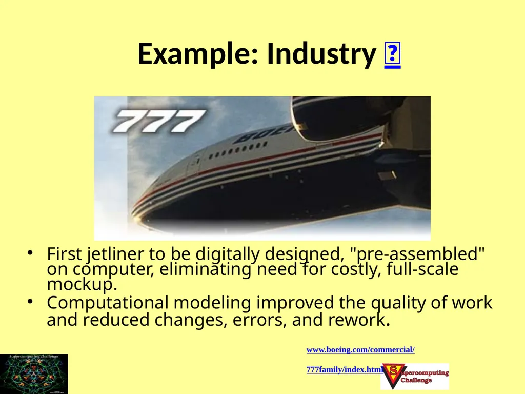
slide6. Example: Industry First jetliner to be digitally designed, "pre-assembled" on computer, eliminating need for costly, full-scale mockup.
Computational modeling improved the quality of work and reduced changes, errors, and rework. www.boeing.com/commercial/
777family/index.html<br>
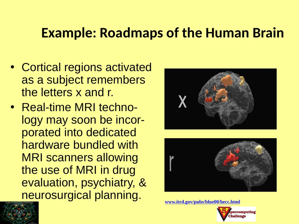
slide7. Example: Roadmaps of the Human Brain Cortical regions activated as a subject remembers the letters x and r.
Real-time MRI techno-logy may soon be incor-porated into dedicated hardware bundled with MRI scanners allowing the use of MRI in drug evaluation, psychiatry, & neurosurgical planning. www.itrd.gov/pubs/blue00/hecc.html<br>
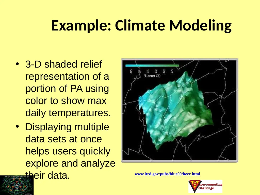
slide8. Example: Climate Modeling 3-D shaded relief representation of a portion of PA using color to show max daily temperatures.
Displaying multiple data sets at once helps users quickly explore and analyze their data. www.itrd.gov/pubs/blue00/hecc.html<br>
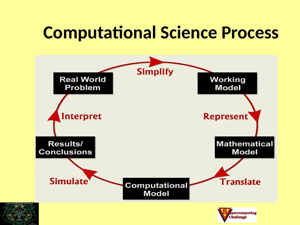
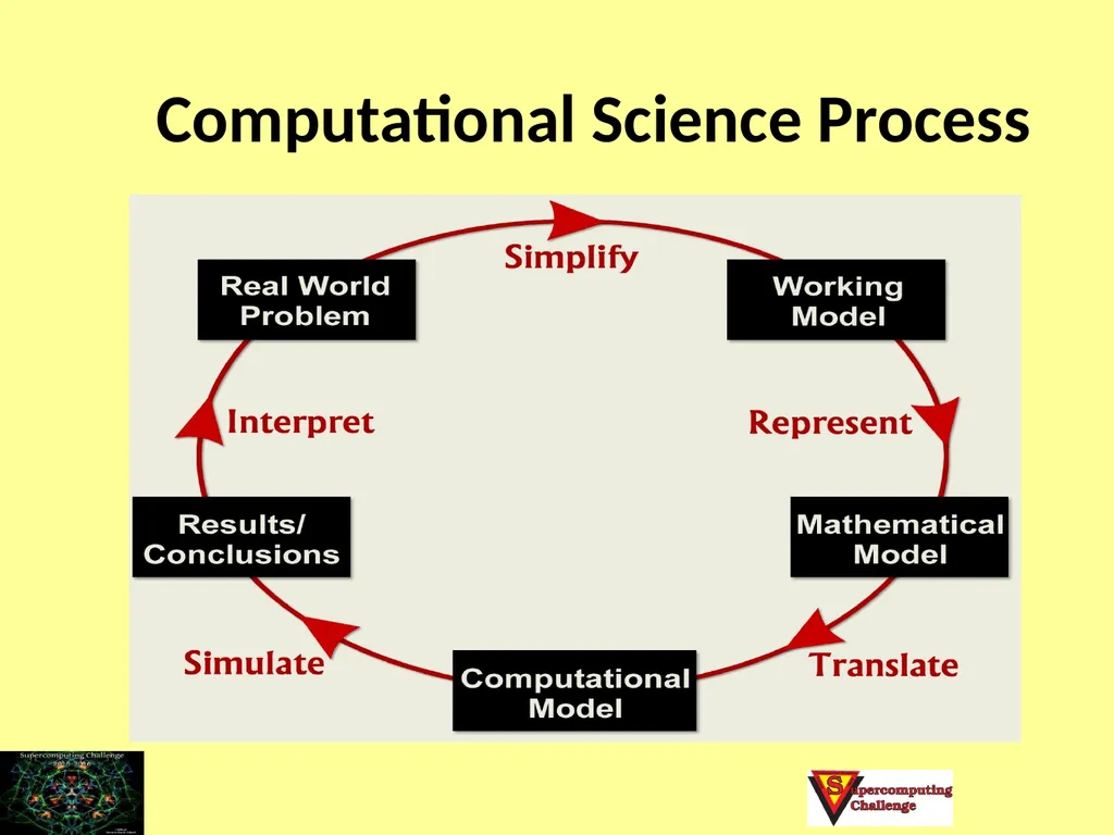
slide9. Computational Science Process<br>
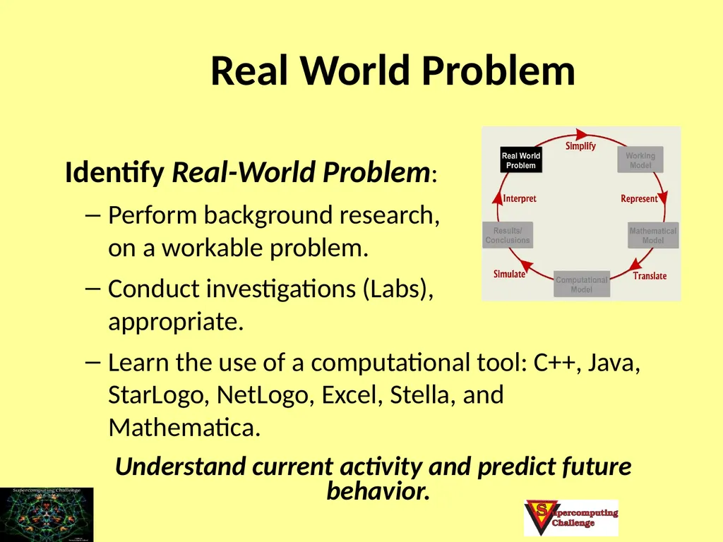
slide10. Real World Problem Identify Real-World Problem:
Perform background research, focus on a workable problem.
Conduct investigations (Labs), if if appropriate.
Learn the use of a computational tool: C++, Java, StarLogo, NetLogo, Excel, Stella, and Mathematica.
Understand current activity and predict future behavior.<br>
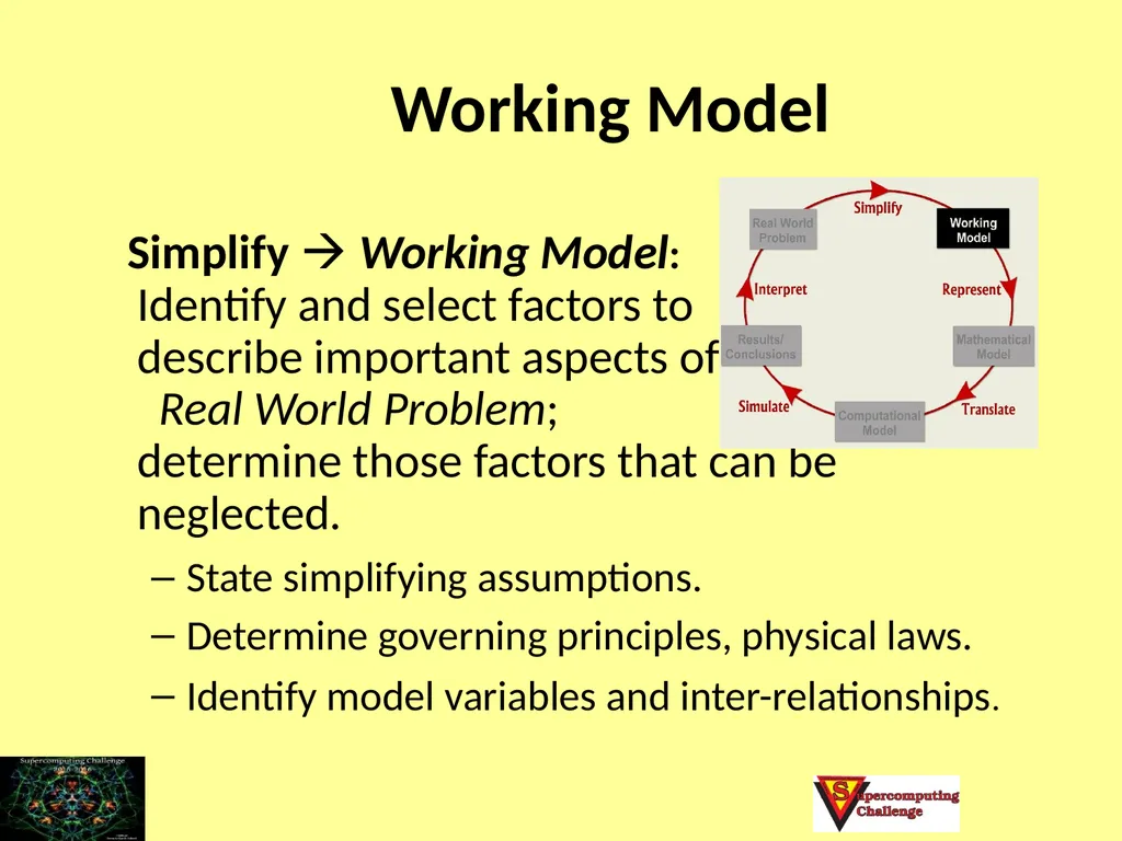
slide11. Working Model Simplify Working Model: Identify and select factors to describe important aspects of Real World Problem; determine those factors that can be neglected.
State simplifying assumptions.
Determine governing principles, physical laws.
Identify model variables and inter-relationships.<br>
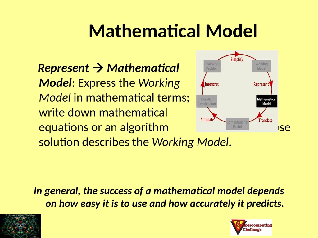
slide12. Mathematical Model Represent Mathematical Model: Express the Working Model in mathematical terms; write down mathematical equations or an algorithm whose solution describes the Working Model.
In general, the success of a mathematical model depends on how easy it is to use and how accurately it predicts.<br>
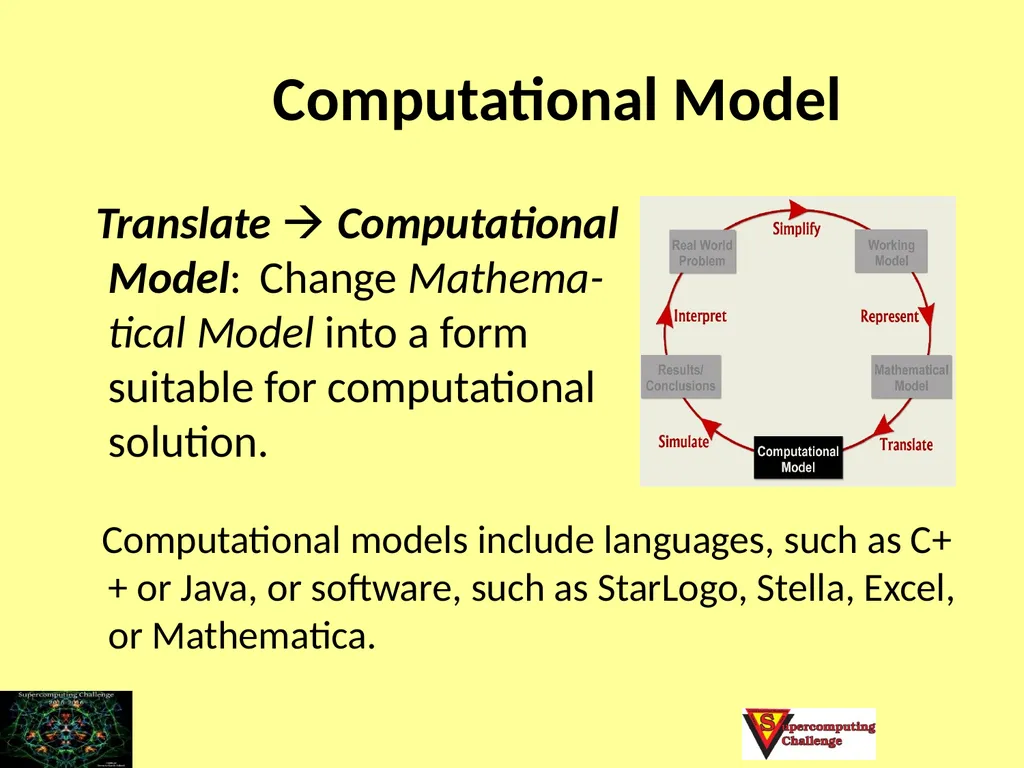
slide13. Computational Model Translate Computational Model: Change Mathema- tical Model into a form suitable for computational solution.
Computational models include languages, such as C++ or Java, or software, such as StarLogo, Stella, Excel, or Mathematica.<br>
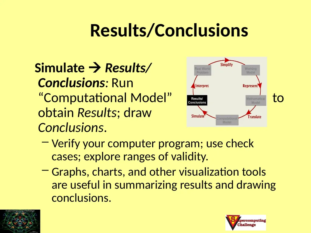
slide14. Results/Conclusions Simulate Results/ Conclusions: Run “Computational Model” to obtain Results; draw Conclusions.
Verify your computer program; use check cases; explore ranges of validity.
Graphs, charts, and other visualization tools are useful in summarizing results and drawing conclusions.<br>
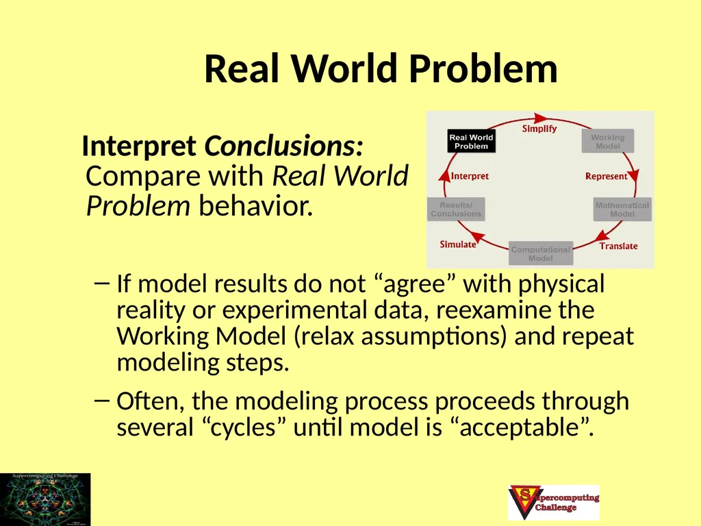
slide15. Real World Problem Interpret Conclusions: Compare with Real World Problem behavior.
If model results do not “agree” with physical reality or experimental data, reexamine the Working Model (relax assumptions) and repeat modeling steps.
Often, the modeling process proceeds through several “cycles” until model is “acceptable”.<br>
slide16. Computational Science Process<br>
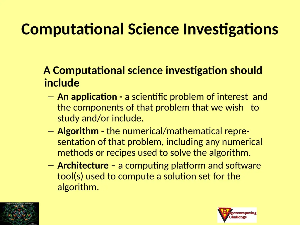
slide17. Computational Science Investigations A Computational science investigation should include
An application - a scientific problem of interest and the components of that problem that we wish to study and/or include.
Algorithm - the numerical/mathematical repre-sentation of that problem, including any numerical methods or recipes used to solve the algorithm.
Architecture – a computing platform and software tool(s) used to compute a solution set for the algorithm.<br>
slide18. Example: A Falling Rock Determine the motion of a rock dropped from a height H, above the ground with initial velocity V.<br>
slide19. Working Model Governing principles: d = v*t and v = a*t.
Simplifying assumptions:
Gravity is the only force acting on the body.
Flat earth.
No drag (air resistance).
Model variables are H,V, g; t, s, and v.<br>
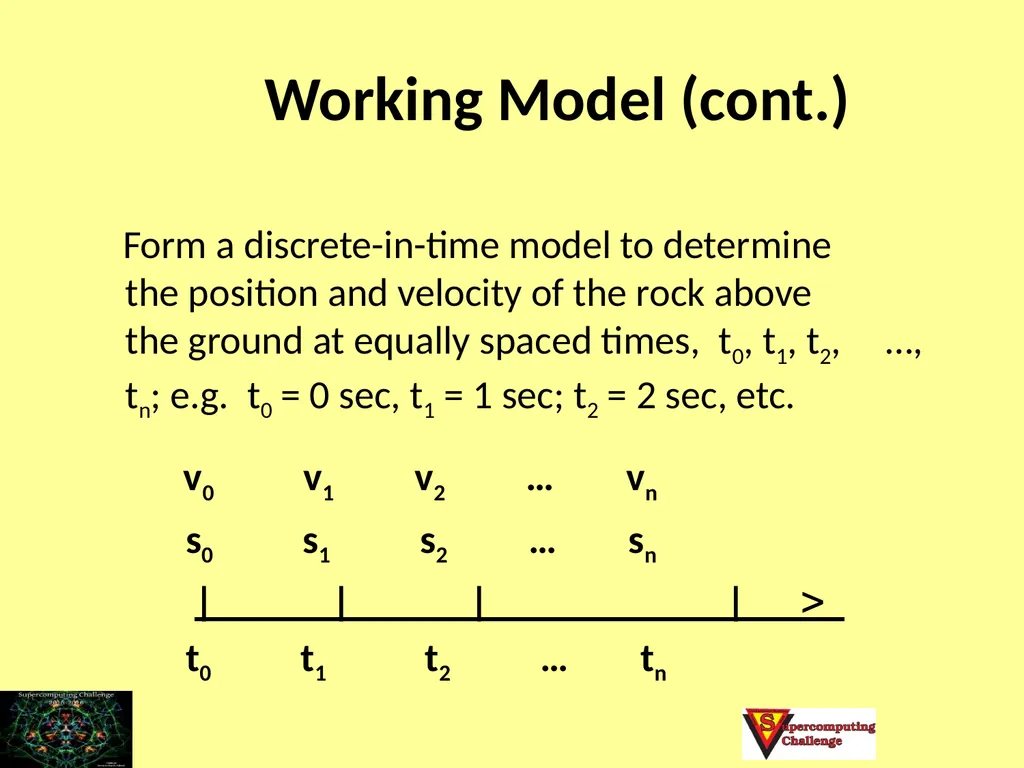
slide20. Working Model (cont.) Form a discrete-in-time model to determine the position and velocity of the rock above the ground at equally spaced times, t0, t1, t2, …, tn; e.g. t0 = 0 sec, t1 = 1 sec; t2 = 2 sec, etc.
v0 v1 v2 … vn
s0 s1 s2 … sn
|______|______|____________|_____
t0 t1 t2 … tn<br>
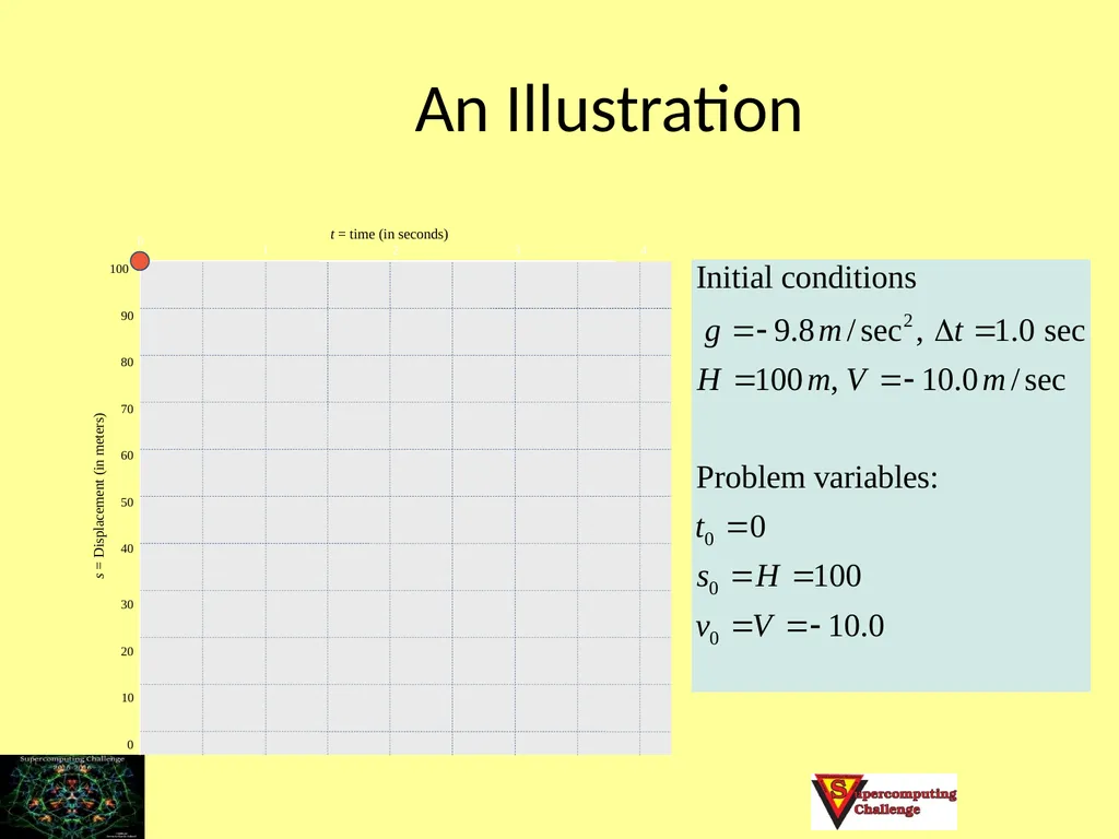
slide21. 100 90 80 70 60 50 40 30 20 s = Displacement (in meters) 10 0 0 1 2 3 4 t = time (in seconds) An Illustration<br>
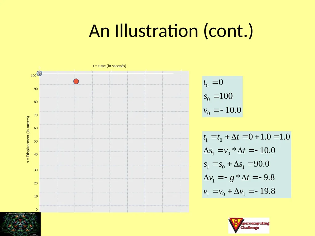
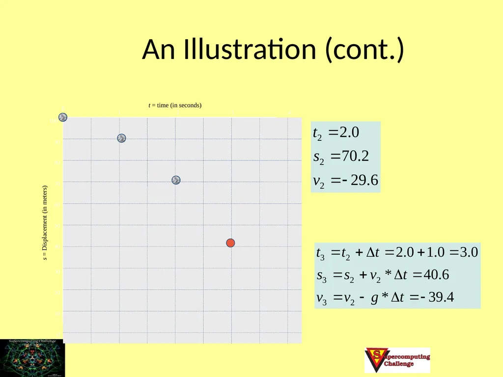
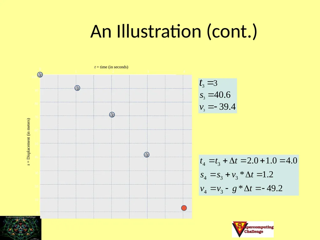
slide22. An Illustration (cont.) 100 90 80 70 60 50 40 30 20 s = Displacement (in meters) 10 0 0 1 2 3 4 t = time (in seconds)<br>
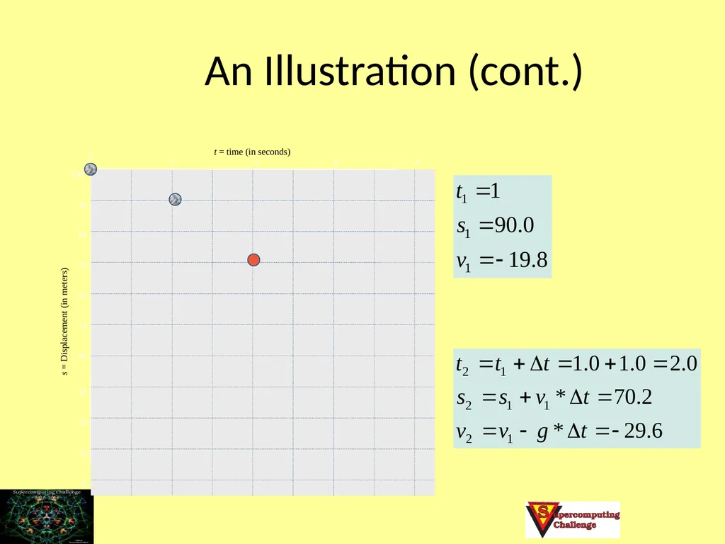
slide23. An Illustration (cont.) 100 90 80 70 60 50 40 30 20 s = Displacement (in meters) 10 0 0 1 2 3 4 t = time (in seconds)<br>
slide24. An Illustration (cont.) 100 90 80 70 60 50 40 30 20 s = Displacement (in meters) 10 0 0 1 2 3 4 t = time (in seconds)<br>
slide25. An Illustration (cont.) 100 90 80 70 60 50 40 30 20 s = Displacement (in meters) 10 0 0 1 2 3 4 t = time (in seconds)<br>
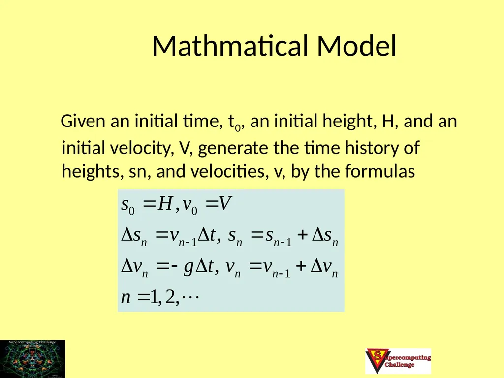
slide26. Mathmatical Model Given an initial time, t0, an initial height, H, and an initial velocity, V, generate the time history of heights, sn, and velocities, v, by the formulas<br>
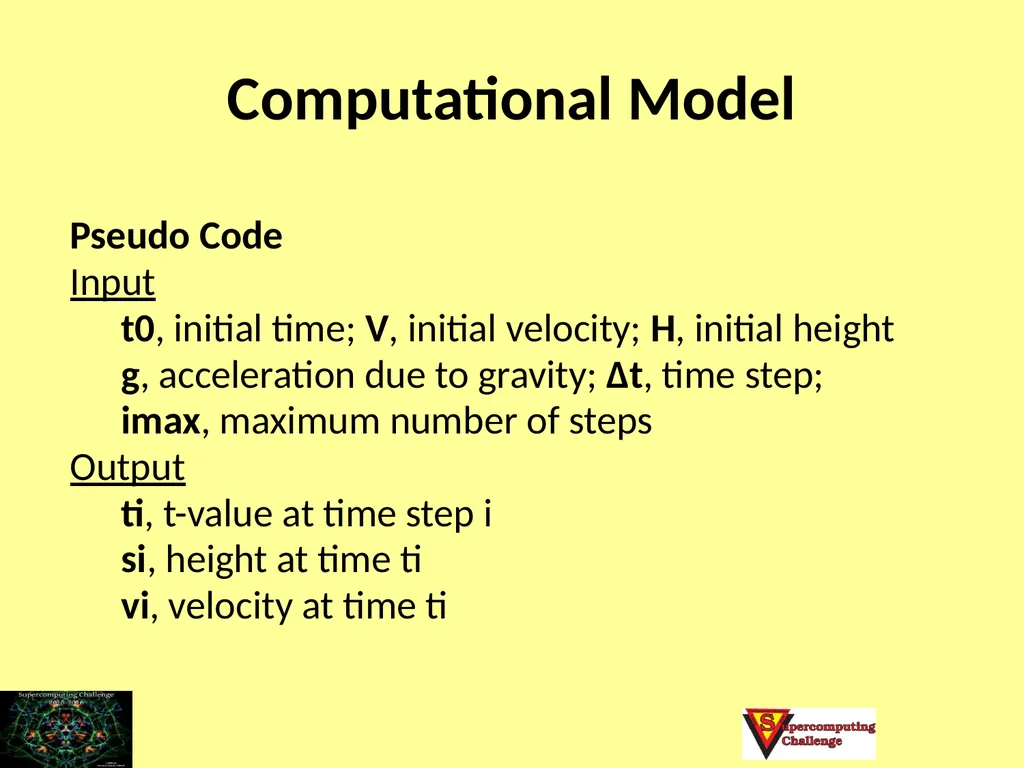
slide27. Computational Model Pseudo Code
Input
t0, initial time; V, initial velocity; H, initial height
g, acceleration due to gravity; Δt, time step;
imax, maximum number of steps
Output
ti, t-value at time step i
si, height at time ti
vi, velocity at time ti<br>
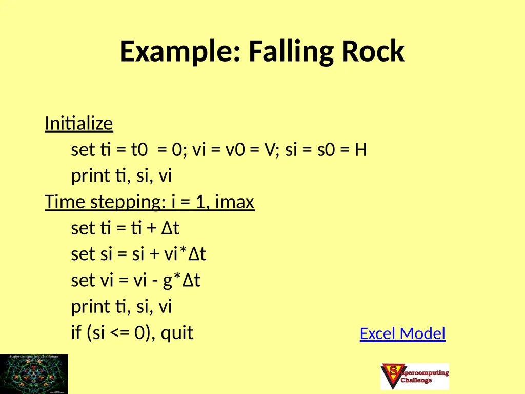
slide28. Example: Falling Rock Initialize
set ti = t0 = 0; vi = v0 = V; si = s0 = H
print ti, si, vi
Time stepping: i = 1, imax
set ti = ti + Δt
set si = si + vi*Δt
set vi = vi - g*Δt
print ti, si, vi
if (si <= 0), quit Excel Model<br>
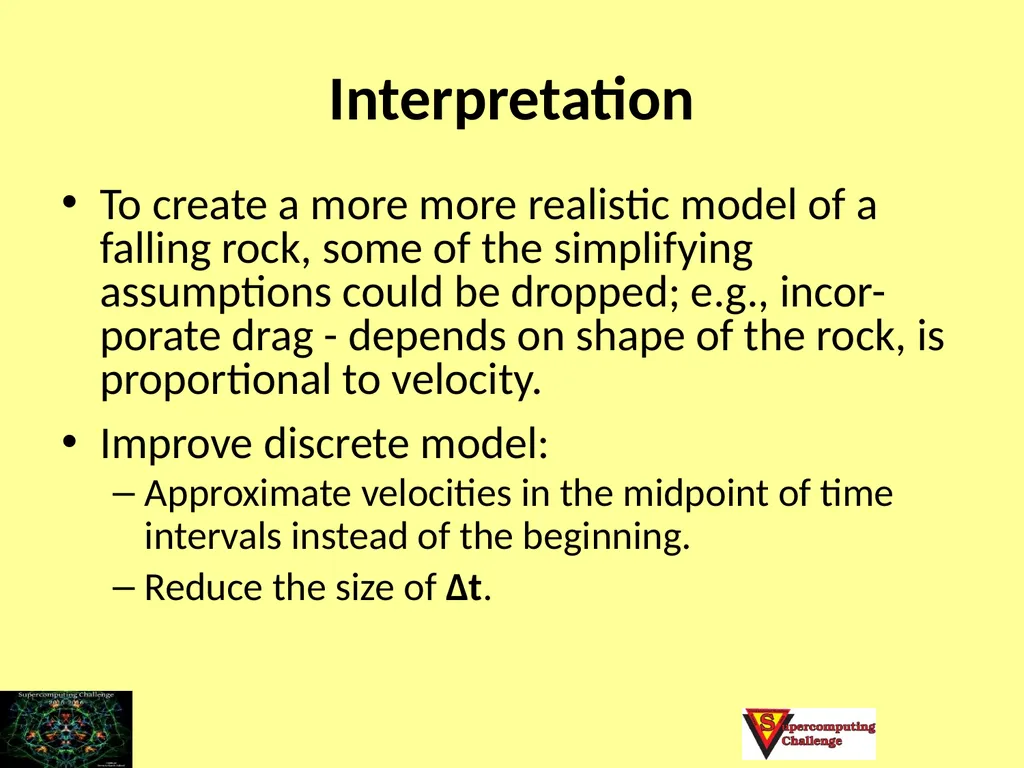
slide29. Interpretation To create a more more realistic model of a falling rock, some of the simplifying assumptions could be dropped; e.g., incor-porate drag - depends on shape of the rock, is proportional to velocity.
Improve discrete model:
Approximate velocities in the midpoint of time intervals instead of the beginning.
Reduce the size of Δt.<br>
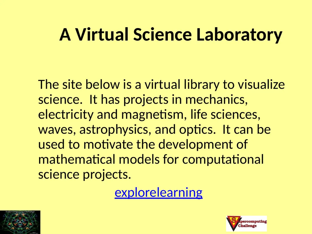
slide30. A Virtual Science Laboratory The site below is a virtual library to visualize science. It has projects in mechanics, electricity and magnetism, life sciences, waves, astrophysics, and optics. It can be used to motivate the development of mathematical models for computational science projects.
explorelearning<br>
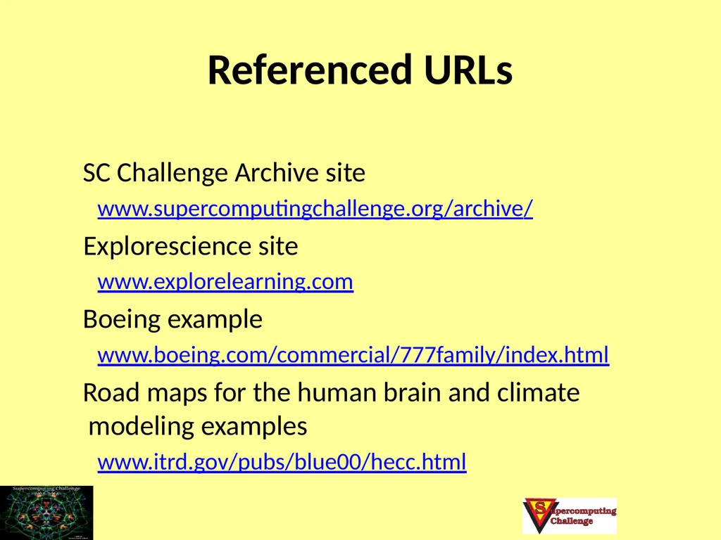
slide31. Referenced URLs SC Challenge Archive site
www.supercomputingchallenge.org/archive/
Explorescience site
www.explorelearning.com
Boeing example
www.boeing.com/commercial/777family/index.html
Road maps for the human brain and climate modeling examples
www.itrd.gov/pubs/blue00/hecc.html<br>
slide32. An interesting modeling site Formulating models
www.cnr.colostate.edu/class_info/nr575/webfiles/L05_Formulating_Continuous_Time_Models.pdf
Falling bodies
http://hypertextbook.com/physics/mechanics/falling/
Master tools
http://www.shodor.org/master/<br>

slide2. Computational Science? Computational science seeks to gain an
understanding of science through the use of
mathematical models on supercomputers. Computational Science involves teamwork<br>
slide3. Computational Science Complements, but does not replace, theory and experimentation in scientific research.<br>
slide4. Computational Science Is often used in place of experiments when experiments are too large, too expensive, too dangerous, or too time consuming.
Can be useful in “what if” studies; e.g. to investigate the use of pathogens (viruses, bacteria, fungi) to control an insect population.
Is a modern tool for scientific investigation.<br>
slide5. Computational Science Has emerged as a powerful, indispensable tool for studying a variety of problems in scientific research, product and process development, and manufacturing. Seismology
Climate modeling
Economics
Environment
Material research Drug design
Manufacturing
Medicine
Biology Analyze - Predict<br>
slide6. Example: Industry First jetliner to be digitally designed, "pre-assembled" on computer, eliminating need for costly, full-scale mockup.
Computational modeling improved the quality of work and reduced changes, errors, and rework. www.boeing.com/commercial/
777family/index.html<br>
slide7. Example: Roadmaps of the Human Brain Cortical regions activated as a subject remembers the letters x and r.
Real-time MRI techno-logy may soon be incor-porated into dedicated hardware bundled with MRI scanners allowing the use of MRI in drug evaluation, psychiatry, & neurosurgical planning. www.itrd.gov/pubs/blue00/hecc.html<br>
slide8. Example: Climate Modeling 3-D shaded relief representation of a portion of PA using color to show max daily temperatures.
Displaying multiple data sets at once helps users quickly explore and analyze their data. www.itrd.gov/pubs/blue00/hecc.html<br>
slide9. Computational Science Process<br>
slide10. Real World Problem Identify Real-World Problem:
Perform background research, focus on a workable problem.
Conduct investigations (Labs), if if appropriate.
Learn the use of a computational tool: C++, Java, StarLogo, NetLogo, Excel, Stella, and Mathematica.
Understand current activity and predict future behavior.<br>
slide11. Working Model Simplify Working Model: Identify and select factors to describe important aspects of Real World Problem; determine those factors that can be neglected.
State simplifying assumptions.
Determine governing principles, physical laws.
Identify model variables and inter-relationships.<br>
slide12. Mathematical Model Represent Mathematical Model: Express the Working Model in mathematical terms; write down mathematical equations or an algorithm whose solution describes the Working Model.
In general, the success of a mathematical model depends on how easy it is to use and how accurately it predicts.<br>
slide13. Computational Model Translate Computational Model: Change Mathema- tical Model into a form suitable for computational solution.
Computational models include languages, such as C++ or Java, or software, such as StarLogo, Stella, Excel, or Mathematica.<br>
slide14. Results/Conclusions Simulate Results/ Conclusions: Run “Computational Model” to obtain Results; draw Conclusions.
Verify your computer program; use check cases; explore ranges of validity.
Graphs, charts, and other visualization tools are useful in summarizing results and drawing conclusions.<br>
slide15. Real World Problem Interpret Conclusions: Compare with Real World Problem behavior.
If model results do not “agree” with physical reality or experimental data, reexamine the Working Model (relax assumptions) and repeat modeling steps.
Often, the modeling process proceeds through several “cycles” until model is “acceptable”.<br>
slide16. Computational Science Process<br>
slide17. Computational Science Investigations A Computational science investigation should include
An application - a scientific problem of interest and the components of that problem that we wish to study and/or include.
Algorithm - the numerical/mathematical repre-sentation of that problem, including any numerical methods or recipes used to solve the algorithm.
Architecture – a computing platform and software tool(s) used to compute a solution set for the algorithm.<br>
slide18. Example: A Falling Rock Determine the motion of a rock dropped from a height H, above the ground with initial velocity V.<br>
slide19. Working Model Governing principles: d = v*t and v = a*t.
Simplifying assumptions:
Gravity is the only force acting on the body.
Flat earth.
No drag (air resistance).
Model variables are H,V, g; t, s, and v.<br>
slide20. Working Model (cont.) Form a discrete-in-time model to determine the position and velocity of the rock above the ground at equally spaced times, t0, t1, t2, …, tn; e.g. t0 = 0 sec, t1 = 1 sec; t2 = 2 sec, etc.
v0 v1 v2 … vn
s0 s1 s2 … sn
|______|______|____________|_____
t0 t1 t2 … tn<br>
slide21. 100 90 80 70 60 50 40 30 20 s = Displacement (in meters) 10 0 0 1 2 3 4 t = time (in seconds) An Illustration<br>
slide22. An Illustration (cont.) 100 90 80 70 60 50 40 30 20 s = Displacement (in meters) 10 0 0 1 2 3 4 t = time (in seconds)<br>
slide23. An Illustration (cont.) 100 90 80 70 60 50 40 30 20 s = Displacement (in meters) 10 0 0 1 2 3 4 t = time (in seconds)<br>
slide24. An Illustration (cont.) 100 90 80 70 60 50 40 30 20 s = Displacement (in meters) 10 0 0 1 2 3 4 t = time (in seconds)<br>
slide25. An Illustration (cont.) 100 90 80 70 60 50 40 30 20 s = Displacement (in meters) 10 0 0 1 2 3 4 t = time (in seconds)<br>
slide26. Mathmatical Model Given an initial time, t0, an initial height, H, and an initial velocity, V, generate the time history of heights, sn, and velocities, v, by the formulas<br>
slide27. Computational Model Pseudo Code
Input
t0, initial time; V, initial velocity; H, initial height
g, acceleration due to gravity; Δt, time step;
imax, maximum number of steps
Output
ti, t-value at time step i
si, height at time ti
vi, velocity at time ti<br>
slide28. Example: Falling Rock Initialize
set ti = t0 = 0; vi = v0 = V; si = s0 = H
print ti, si, vi
Time stepping: i = 1, imax
set ti = ti + Δt
set si = si + vi*Δt
set vi = vi - g*Δt
print ti, si, vi
if (si <= 0), quit Excel Model<br>
slide29. Interpretation To create a more more realistic model of a falling rock, some of the simplifying assumptions could be dropped; e.g., incor-porate drag - depends on shape of the rock, is proportional to velocity.
Improve discrete model:
Approximate velocities in the midpoint of time intervals instead of the beginning.
Reduce the size of Δt.<br>
slide30. A Virtual Science Laboratory The site below is a virtual library to visualize science. It has projects in mechanics, electricity and magnetism, life sciences, waves, astrophysics, and optics. It can be used to motivate the development of mathematical models for computational science projects.
explorelearning<br>
slide31. Referenced URLs SC Challenge Archive site
www.supercomputingchallenge.org/archive/
Explorescience site
www.explorelearning.com
Boeing example
www.boeing.com/commercial/777family/index.html
Road maps for the human brain and climate modeling examples
www.itrd.gov/pubs/blue00/hecc.html<br>
slide32. An interesting modeling site Formulating models
www.cnr.colostate.edu/class_info/nr575/webfiles/L05_Formulating_Continuous_Time_Models.pdf
Falling bodies
http://hypertextbook.com/physics/mechanics/falling/
Master tools
http://www.shodor.org/master/<br>