Aggregate Demand II: Applying the IS-LM Model 12

slide1. Aggregate Demand II:
Applying the IS-LM Model 12<br>
slide2. Context Chapter 10 introduced the model of aggregate demand and supply.
Chapter 11 developed the IS-LM model, the basis of the aggregate demand curve.<br>
slide3. IN THIS CHAPTER, YOU WILL LEARN: how to use the IS-LM model to analyze the effects of shocks, fiscal policy, and monetary policy
how to derive the aggregate demand curve from the IS-LM model
several theories about what caused the Great Depression 2<br>
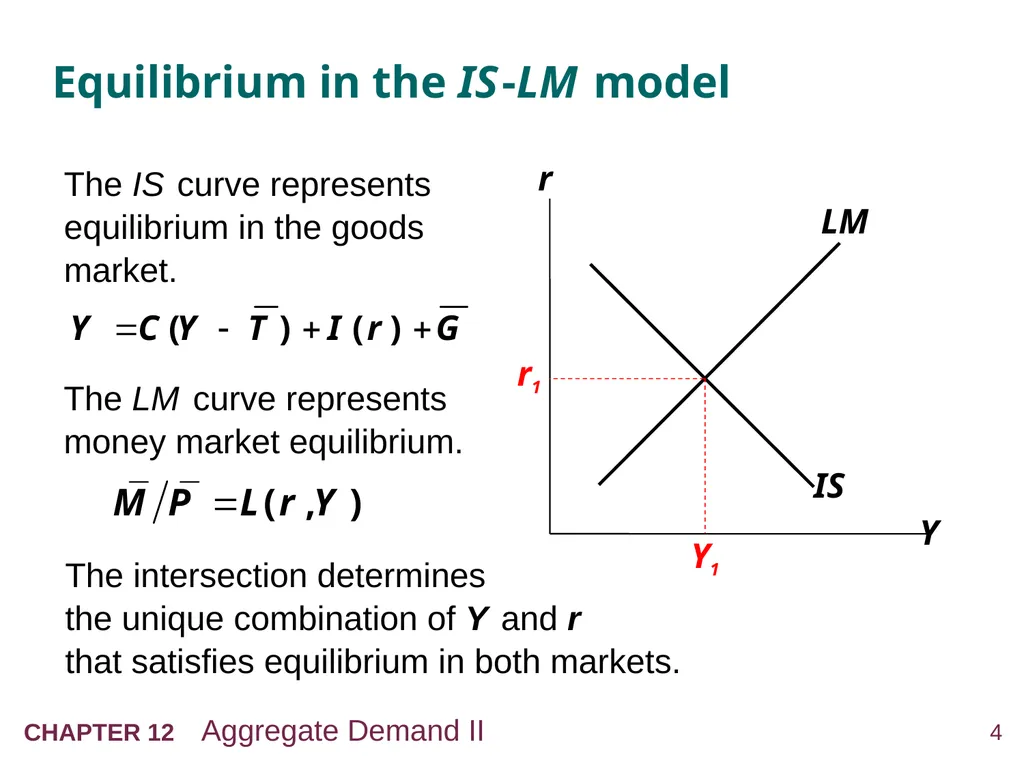
slide4. The intersection determines the unique combination of Y and r that satisfies equilibrium in both markets. The LM curve represents money market equilibrium. Equilibrium in the IS -LM model The IS curve represents equilibrium in the goods market. r1 Y1<br>
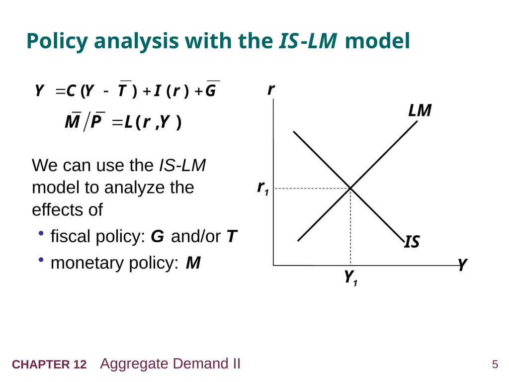
slide5. Policy analysis with the IS -LM model We can use the IS-LM model to analyze the effects of
fiscal policy: G and/or T
monetary policy: M<br>
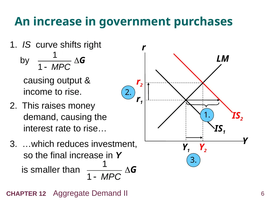
slide6. causing output & income to rise. An increase in government purchases 1. IS curve shifts right 2. This raises money demand, causing the interest rate to rise… 3. …which reduces investment, so the final increase in Y<br>
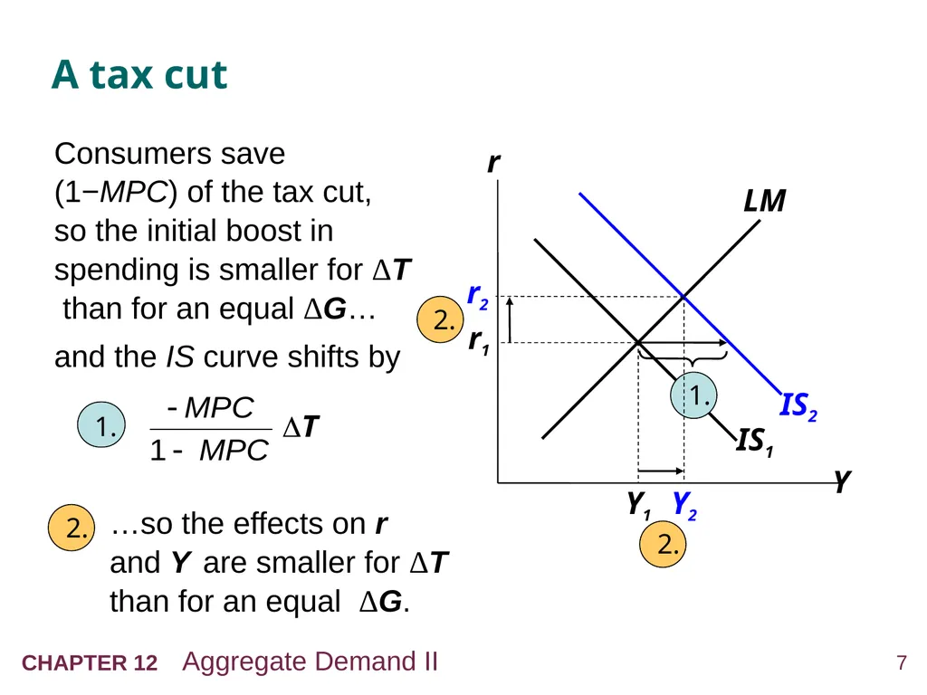
slide7. A tax cut Consumers save (1−MPC) of the tax cut, so the initial boost in spending is smaller for ΔT than for an equal ΔG…
and the IS curve shifts by …so the effects on r and Y are smaller for ΔT than for an equal ΔG.<br>
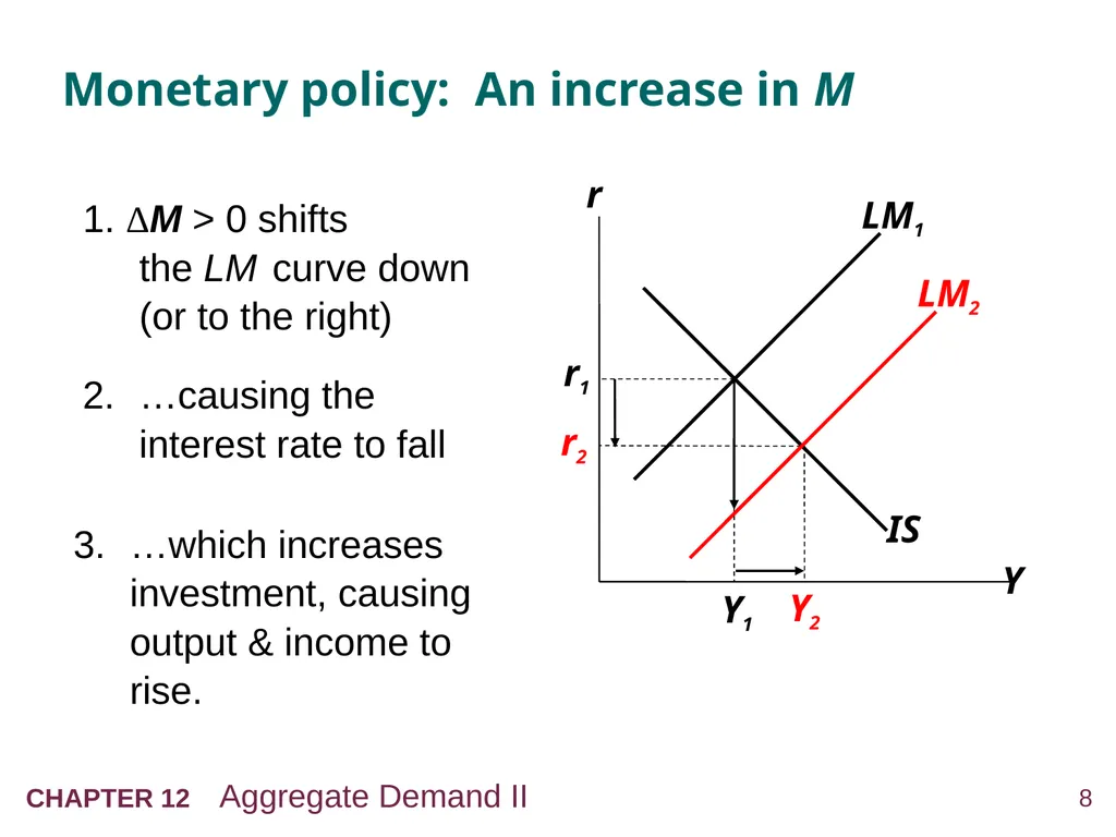
slide8. 2. …causing the interest rate to fall Monetary policy: An increase in M 1. ΔM > 0 shifts the LM curve down(or to the right) 3. …which increases investment, causing output & income to rise.<br>
slide9. Interaction between monetary & fiscal policy Model:
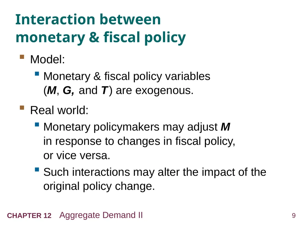
Monetary & fiscal policy variables (M, G, and T ) are exogenous.
Real world:
Monetary policymakers may adjust M in response to changes in fiscal policy, or vice versa.
Such interactions may alter the impact of the original policy change.<br>
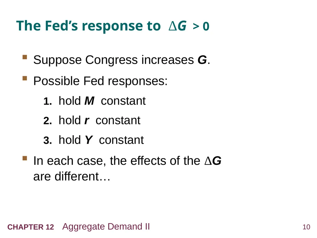
slide10. The Fed’s response to ΔG > 0 Suppose Congress increases G.
Possible Fed responses:
1. hold M constant
2. hold r constant
3. hold Y constant
In each case, the effects of the ΔG are different…<br>
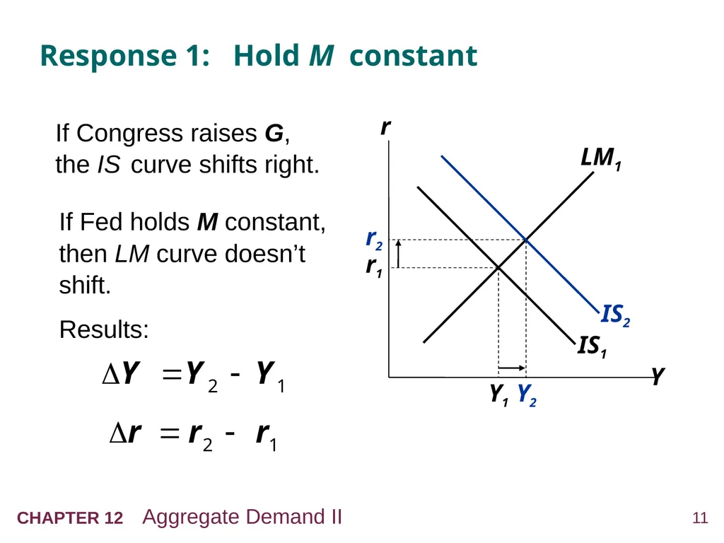
slide11. If Congress raises G, the IS curve shifts right. Response 1: Hold M constant If Fed holds M constant, then LM curve doesn’t shift.
Results:<br>
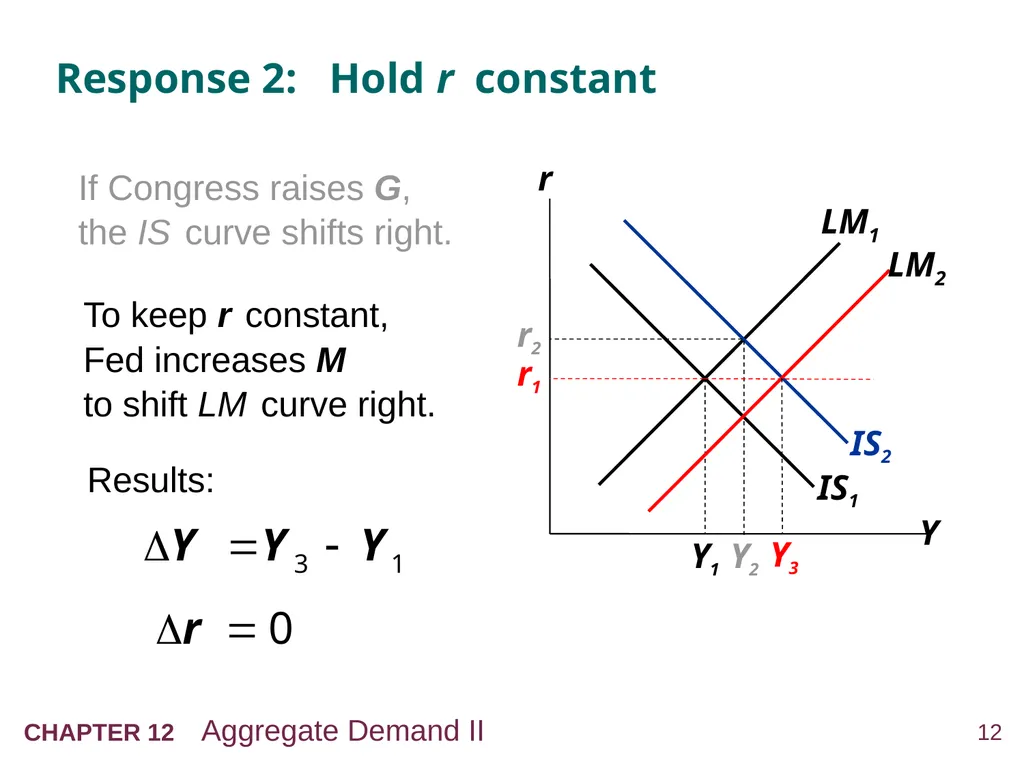
slide12. If Congress raises G, the IS curve shifts right. Response 2: Hold r constant r1 r2 To keep r constant, Fed increases M to shift LM curve right. Results:<br>
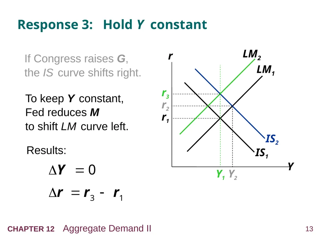
slide13. Response 3: Hold Y constant r2 To keep Y constant, Fed reduces M to shift LM curve left. Results: If Congress raises G, the IS curve shifts right.<br>
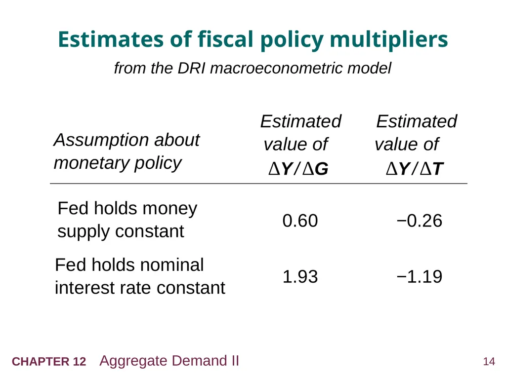
slide14. Estimates of fiscal policy multipliers from the DRI macroeconometric model Assumption about monetary policy Estimated value of ΔY / ΔG Fed holds nominal interest rate constant Fed holds money supply constant 1.93 0.60 Estimated value of ΔY / ΔT −1.19 −0.26<br>
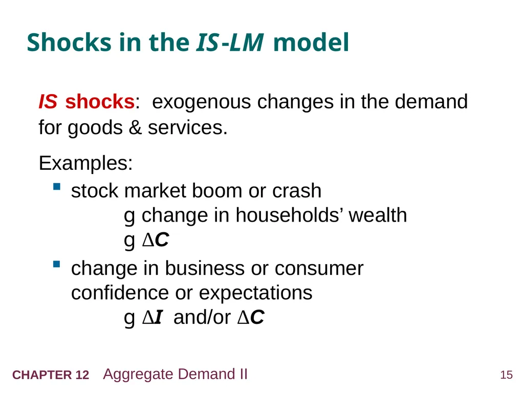
slide15. Shocks in the IS -LM model IS shocks: exogenous changes in the demand for goods & services.
Examples:
stock market boom or crash g change in households’ wealth g ΔC
change in business or consumer confidence or expectations  g ΔI and/or ΔC<br>
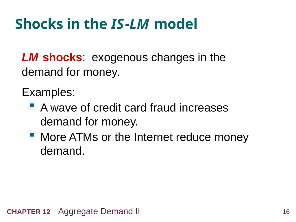
slide16. Shocks in the IS -LM model LM shocks: exogenous changes in the demand for money.
Examples:
A wave of credit card fraud increases demand for money.
More ATMs or the Internet reduce money demand.<br>
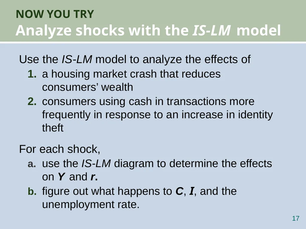
slide17. NOW YOU TRYAnalyze shocks with the IS-LM model Use the IS-LM model to analyze the effects of
1. a housing market crash that reduces consumers’ wealth
2. consumers using cash in transactions more frequently in response to an increase in identity theft
For each shock,
a. use the IS-LM diagram to determine the effects on Y and r.
b. figure out what happens to C, I, and the unemployment rate. 16<br>
slide18. ANSWERS, PART 1Housing market crash 17 IS shifts left, causing
r and Y to fall.

C falls due to lower wealth and lower income,
I rises because r is lower
u rises because Y is lower (Okun’s law)<br>
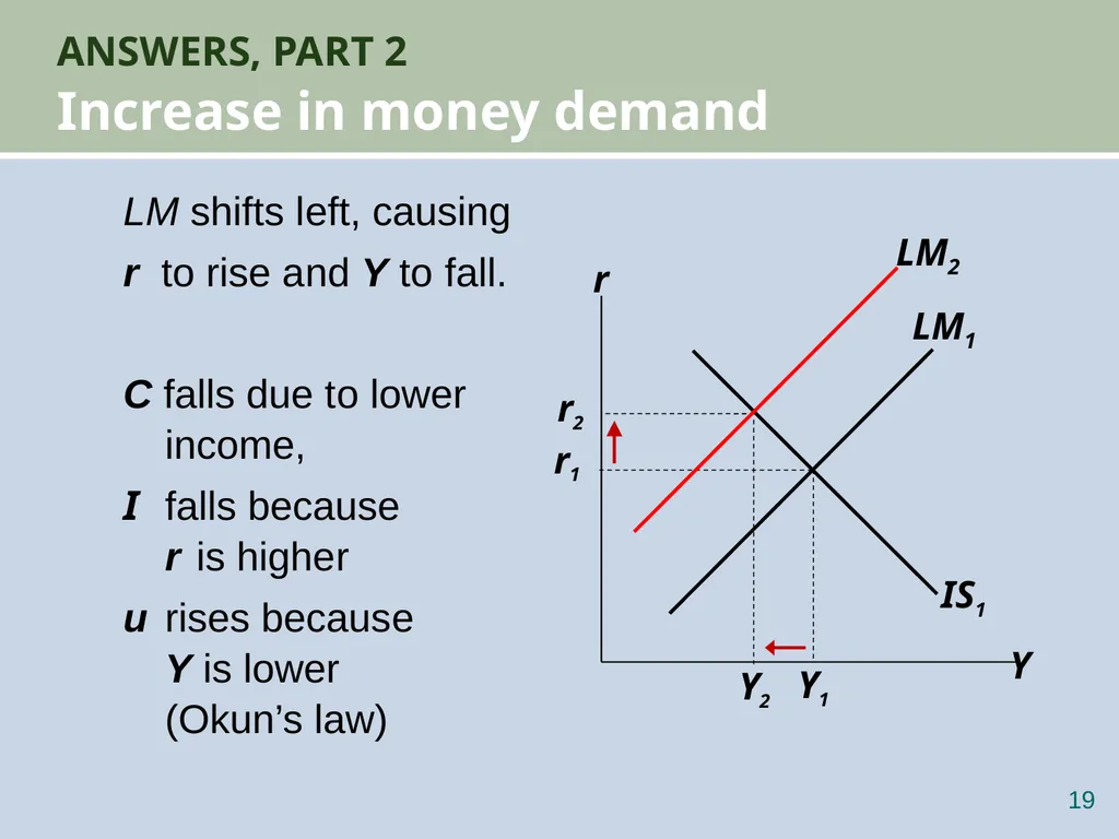
slide19. ANSWERS, PART 2Increase in money demand 18 LM shifts left, causing
r to rise and Y to fall.

C falls due to lower income,
I falls because r is higher
u rises because Y is lower (Okun’s law)<br>
slide20. CASE STUDY: The U.S. recession of 2001 During 2001:
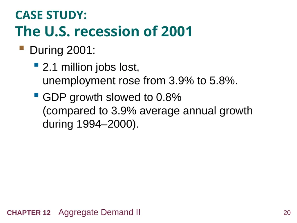
2.1 million jobs lost, unemployment rose from 3.9% to 5.8%.
GDP growth slowed to 0.8% (compared to 3.9% average annual growth during 1994–2000).<br>
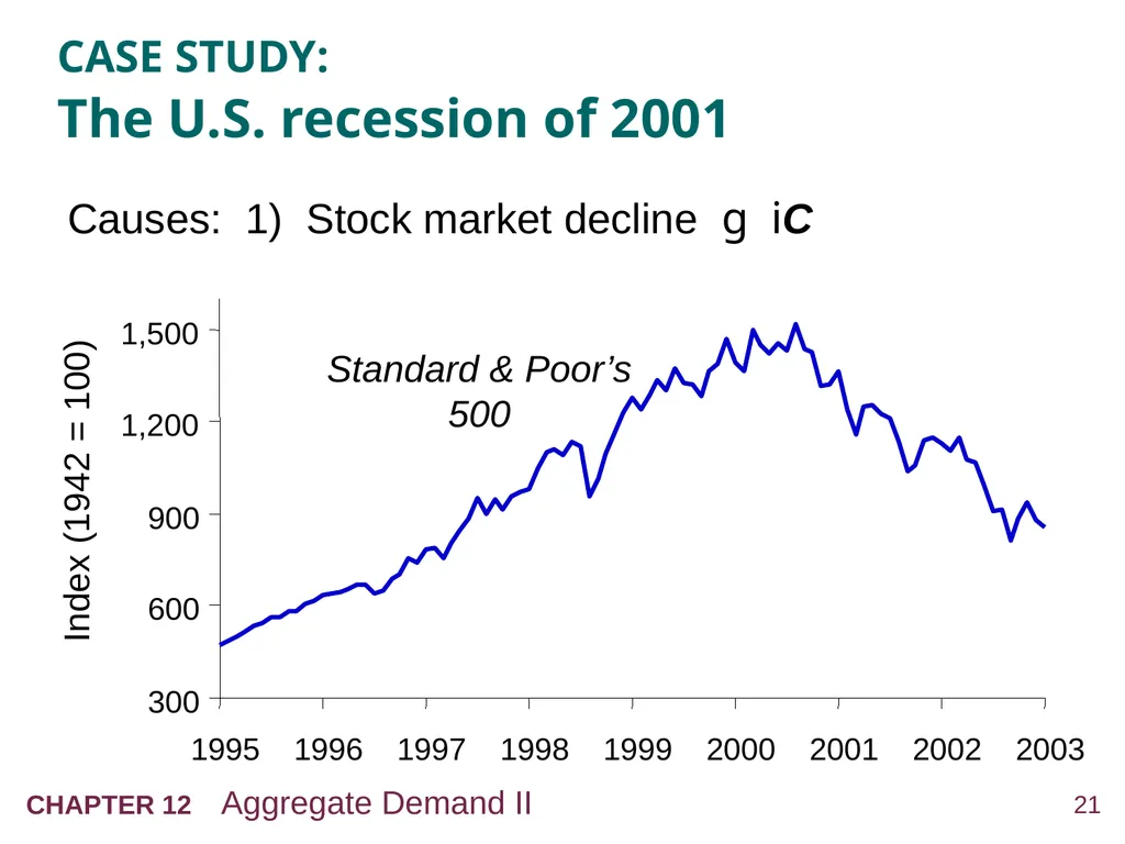
slide21. CASE STUDY: The U.S. recession of 2001 Causes: 1) Stock market decline g iC<br>
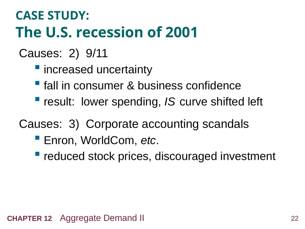
slide22. CASE STUDY: The U.S. recession of 2001 Causes: 2) 9/11
increased uncertainty
fall in consumer & business confidence
result: lower spending, IS curve shifted left
Causes: 3) Corporate accounting scandals
Enron, WorldCom, etc.
reduced stock prices, discouraged investment<br>
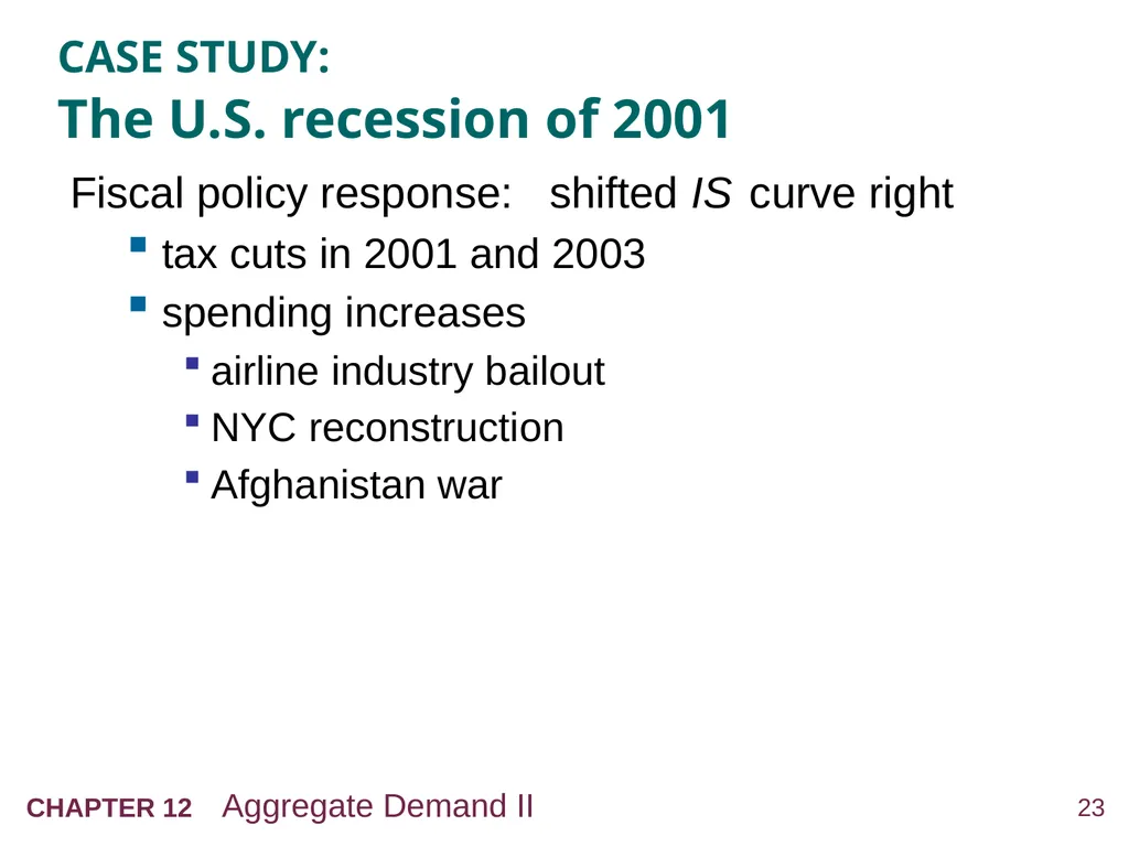
slide23. CASE STUDY: The U.S. recession of 2001 Fiscal policy response: shifted IS curve right
tax cuts in 2001 and 2003
spending increases
airline industry bailout
NYC reconstruction
Afghanistan war<br>
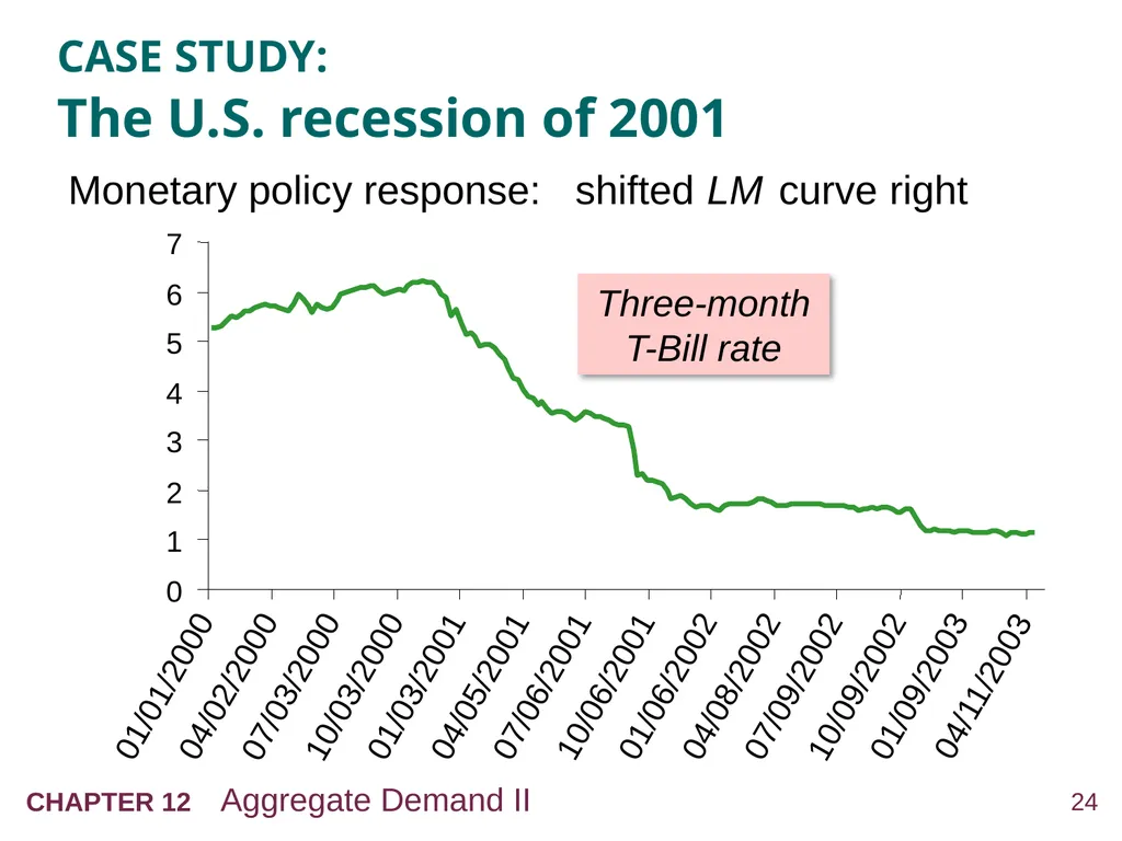
slide24. CASE STUDY: The U.S. recession of 2001 Monetary policy response: shifted LM curve right<br>
slide25. What is the Fed’s policy instrument? The news media commonly report the Fed’s policy changes as interest rate changes, as if the Fed has direct control over market interest rates.
In fact, the Fed targets the federal funds rate—the interest rate banks charge one another on overnight loans.
The Fed changes the money supply and shifts the LM curve to achieve its target.
Other short-term rates typically move with the federal funds rate.<br>
slide26. What is the Fed’s policy instrument? Why does the Fed target interest rates instead of the money supply?
1) They are easier to measure than the money supply.
2) The Fed might believe that LM shocks are more prevalent than IS shocks. If so, then targeting the interest rate stabilizes income better than targeting the money supply. (See problem 7 on p.353.)<br>
slide27. IS-LM and aggregate demand So far, we’ve been using the IS-LM model to analyze the short run, when the price level is assumed fixed.
However, a change in P would shift LM and therefore affect Y.
The aggregate demand curve (introduced in Chap. 10) captures this relationship between P and Y.<br>
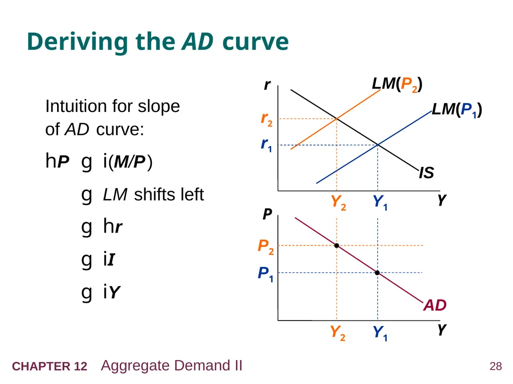
slide28. Y1 Y2 Deriving the AD curve AD Y2 Y1 Intuition for slope of AD curve:
hP g i(M/P )
g LM shifts left
g hr
g iI
g iY<br>
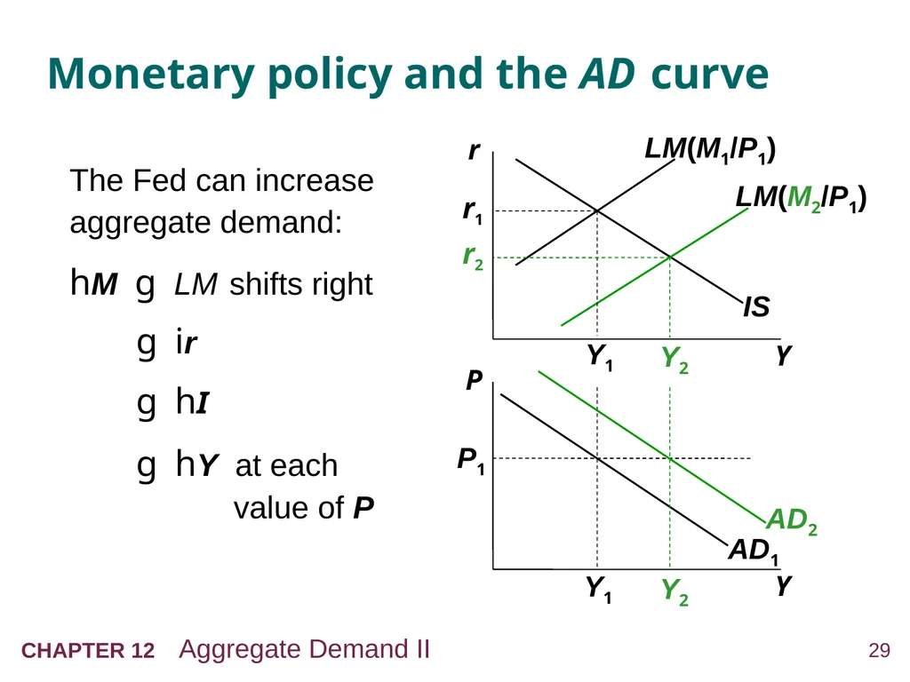
slide29. Monetary policy and the AD curve The Fed can increase aggregate demand:
hM g LM shifts right g ir g hI
g hY at each value of P<br>
slide30. Fiscal policy and the AD curve Expansionary fiscal policy (hG and/or iT ) increases agg. demand:
iT g hC
g IS shifts right
g hY at each value of P<br>
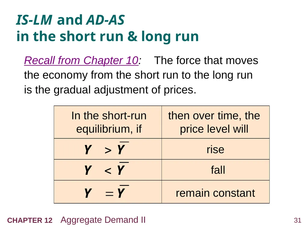
slide31. IS-LM and AD-AS in the short run & long run Recall from Chapter 10: The force that moves the economy from the short run to the long run is the gradual adjustment of prices. rise fall remain constant In the short-run equilibrium, if then over time, the price level will<br>
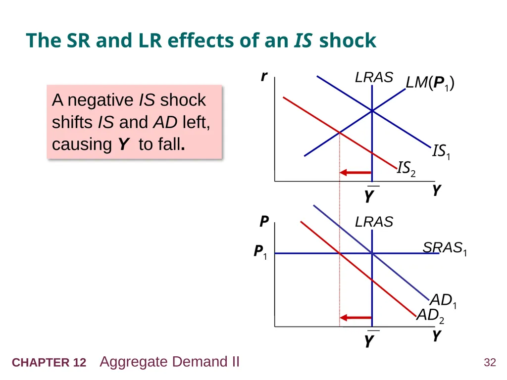
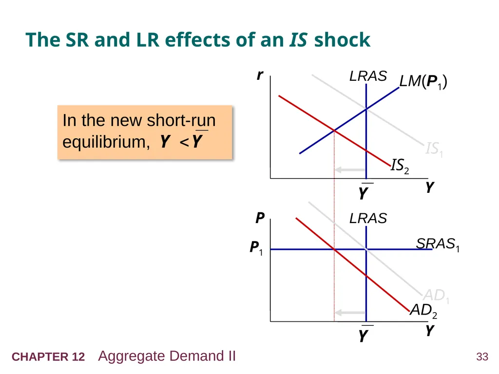
slide32. The SR and LR effects of an IS shock A negative IS shock shifts IS and AD left, causing Y to fall.<br>
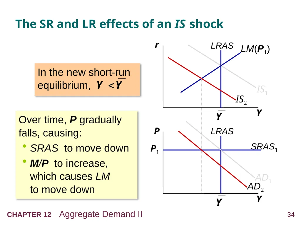
slide33. The SR and LR effects of an IS shock LRAS IS1 AD1 In the new short-run equilibrium,<br>
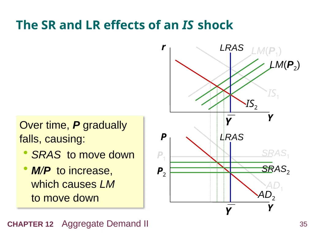
slide34. The SR and LR effects of an IS shock LRAS IS1 AD1 In the new short-run equilibrium, Over time, P gradually falls, causing:
SRAS to move down
M/P to increase, which causes LM to move down<br>
slide35. The SR and LR effects of an IS shock LRAS IS1 SRAS1 P1 LM(P1) AD1 Over time, P gradually falls, causing:
SRAS to move down
M/P to increase, which causes LM to move down<br>
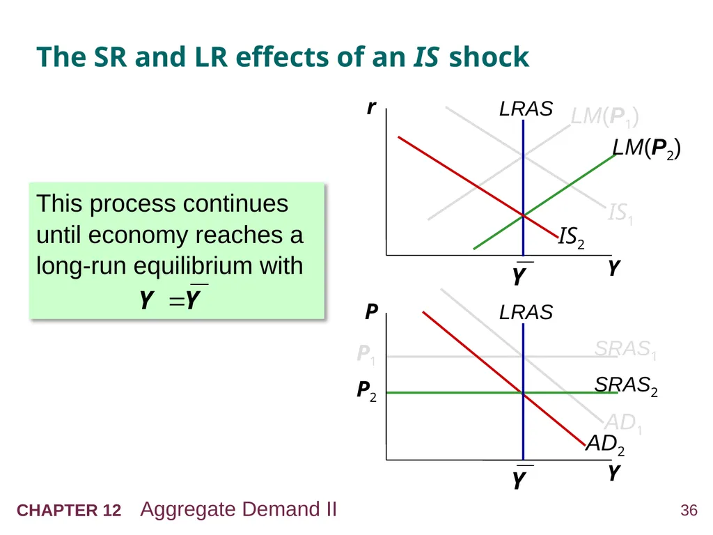
slide36. The SR and LR effects of an IS shock LRAS IS1 SRAS1 P1 LM(P1) AD1 This process continues until economy reaches a long-run equilibrium with<br>
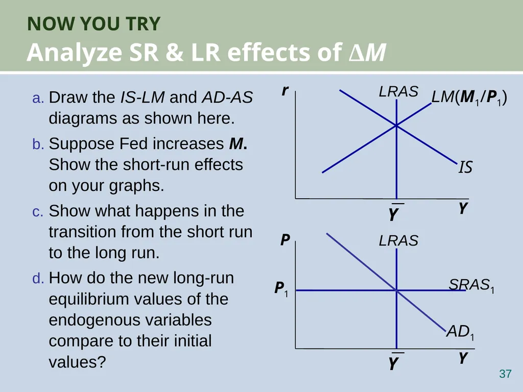
slide37. NOW YOU TRYAnalyze SR & LR effects of ΔM 36 Draw the IS-LM and AD-AS diagrams as shown here.
Suppose Fed increases M. Show the short-run effects on your graphs.
Show what happens in the transition from the short run to the long run.
How do the new long-run equilibrium values of the endogenous variables compare to their initial values? LM(M1/P1)<br>
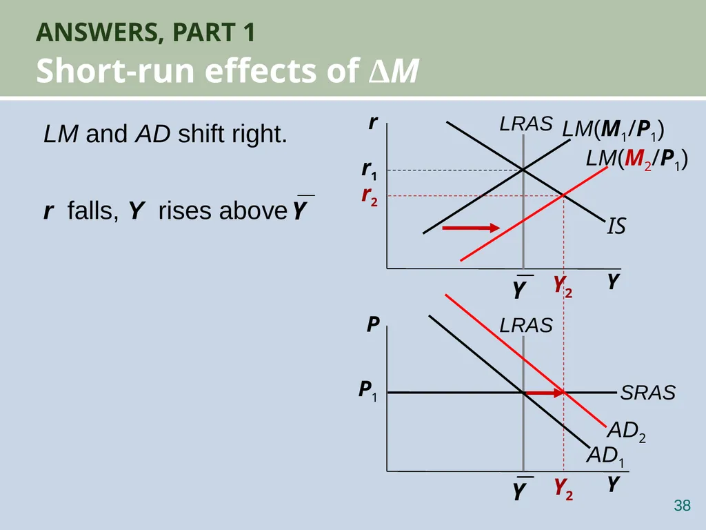
slide38. ANSWERS, PART 1Short-run effects of ΔM 37 LM and AD shift right.

r falls, Y rises above LM(M1/P1) LM(M2/P1) Y2 Y2 r2 r1<br>
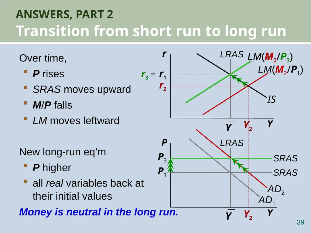
slide39. ANSWERS, PART 2Transition from short run to long run 38 Over time,
P rises
SRAS moves upward
M/P falls
LM moves leftward

New long-run eq’m
P higher
all real variables back at their initial values
Money is neutral in the long run. LM(M1/P1) LM(M2/P1) Y2 Y2 r2 r1 LM(M2/P3) r3 =<br>
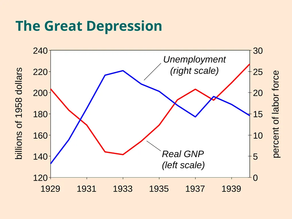
slide40. The Great Depression 120 140 160 180 200 220 240 1929 1931 1933 1935 1937 1939 billions of 1958 dollars 0 5 10 15 20 25 30 percent of labor force<br>
slide41. THE SPENDING HYPOTHESIS: Shocks to the IS curve Asserts the Depression was largely due to an exogenous fall in the demand for goods & services—a leftward shift of the IS curve.
Evidence: output and interest rates both fell, which is what a leftward IS shift would cause.<br>
slide42. THE SPENDING HYPOTHESIS: Reasons for the IS shift Stock market crash reduced consumption
Oct 1929–Dec 1929: S&P 500 fell 17%
Oct 1929–Dec 1933: S&P 500 fell 71%
Drop in investment
Correction after overbuilding in the 1920s.
Widespread bank failures made it harder to obtain financing for investment.
Contractionary fiscal policy
Politicians raised tax rates and cut spending to combat increasing deficits.<br>
slide43. THE MONEY HYPOTHESIS: A shock to the LM curve Asserts that the Depression was largely due to huge fall in the money supply.
Evidence: M1 fell 25% during 1929–33.
But, two problems with this hypothesis:
P fell even more, so M/P actually rose slightly during 1929–31.
nominal interest rates fell, which is the opposite of what a leftward LM shift would cause.<br>
slide44. THE MONEY HYPOTHESIS AGAIN: The effects of falling prices Asserts that the severity of the Depression was due to a huge deflation: P fell 25% during 1929–33.
This deflation was probably caused by the fall in M, so perhaps money played an important role after all.
In what ways does a deflation affect the economy?<br>
slide45. THE MONEY HYPOTHESIS AGAIN: The effects of falling prices The stabilizing effects of deflation:
iP g h(M/P) g LM shifts right g hY
Pigou effect:
iP g h(M/P )
g consumers’ wealth h
g hC
g IS shifts right
g hY<br>
slide46. THE MONEY HYPOTHESIS AGAIN: The effects of falling prices The destabilizing effects of expected deflation:
iE π
g r h for each value of i
g I i because I = I (r )
g planned expenditure & agg. demand i
g income & output i<br>
slide47. THE MONEY HYPOTHESIS AGAIN: The effects of falling prices The destabilizing effects of unexpected deflation:debt-deflation theory
iP (if unexpected)
g transfers purchasing power from borrowers to lenders
g borrowers spend less, lenders spend more
g if borrowers’ propensity to spend is larger than lenders’, then aggregate spending falls, the IS curve shifts left, and Y falls<br>
slide48. Why another Depression is unlikely Policymakers (or their advisers) now know much more about macroeconomics:
The Fed knows better than to let M fall so much, especially during a contraction.
Fiscal policymakers know better than to raise taxes or cut spending during a contraction.
Federal deposit insurance makes widespread bank failures very unlikely.
Automatic stabilizers make fiscal policy expansionary during an economic downturn.<br>
slide49. CASE STUDYThe 2008–09 financial crisis & recession 2009: Real GDP fell, u-rate approached 10%
Important factors in the crisis:
early 2000s Federal Reserve interest rate policy
subprime mortgage crisis
bursting of house price bubble, rising foreclosure rates
falling stock prices
failing financial institutions
declining consumer confidence, drop in spending on consumer durables and investment goods<br>
slide50. Interest rates and house prices<br>
slide51. Change in U.S. house price index and rate of new foreclosures, 1999–2009<br>
slide52. House price change and new foreclosures, 2006:Q3–2009:Q1 New foreclosures, % of all mortgages Cumulative change in house price index Nevada Georgia Colorado Texas Alaska Wyoming Arizona California Florida S. Dakota Illinois Michigan Rhode Island N. Dakota Oregon Ohio New Jersey Hawaii<br>
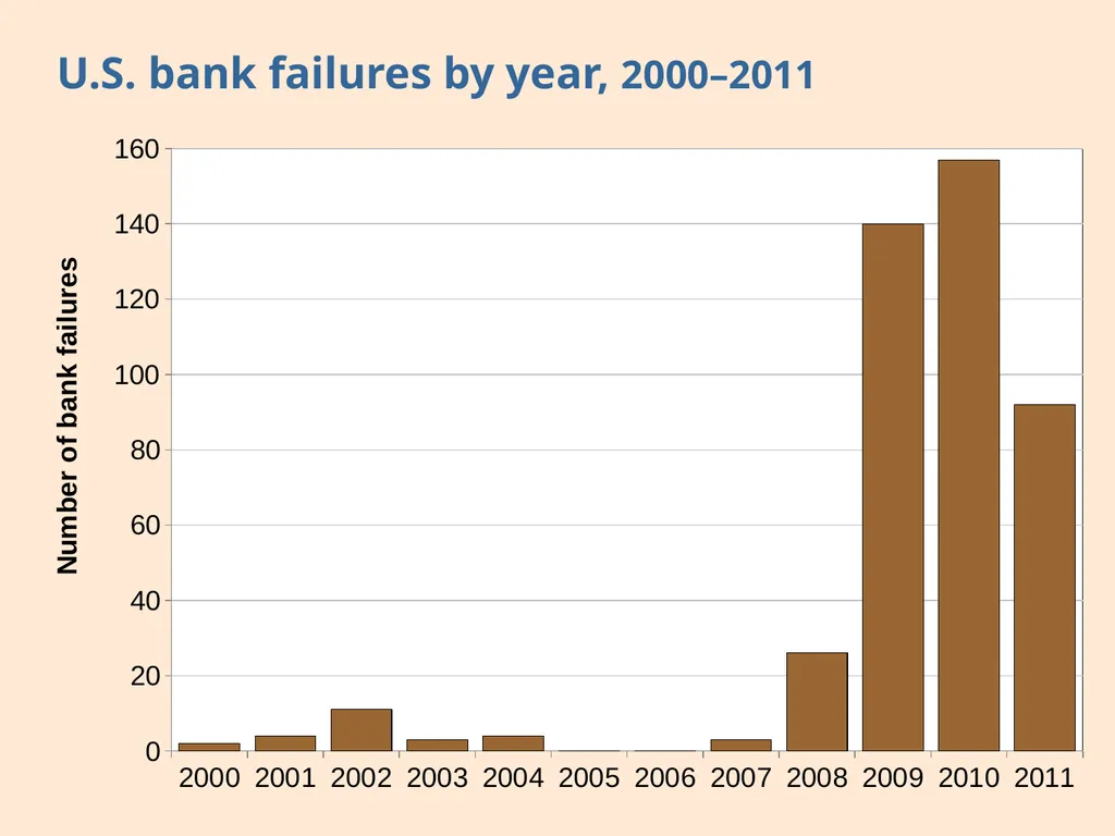
slide53. U.S. bank failures by year, 2000–2011<br>
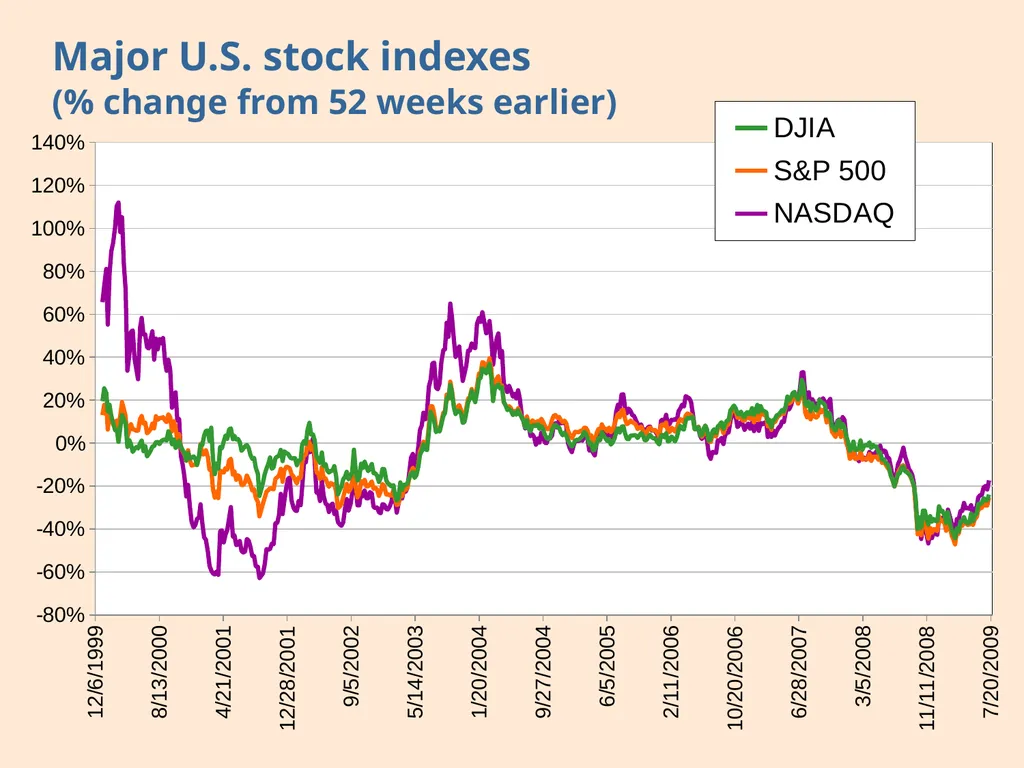
slide54. Major U.S. stock indexes (% change from 52 weeks earlier)<br>
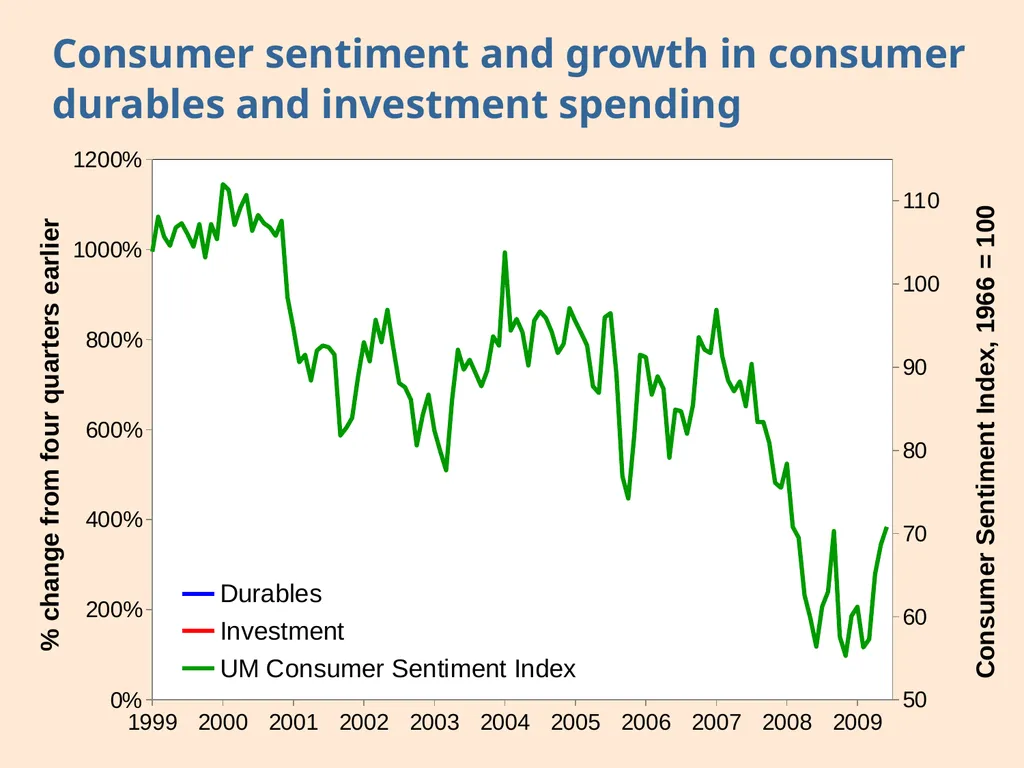
slide55. Consumer sentiment and growth in consumer durables and investment spending<br>
slide56. Real GDP growth and unemployment<br>
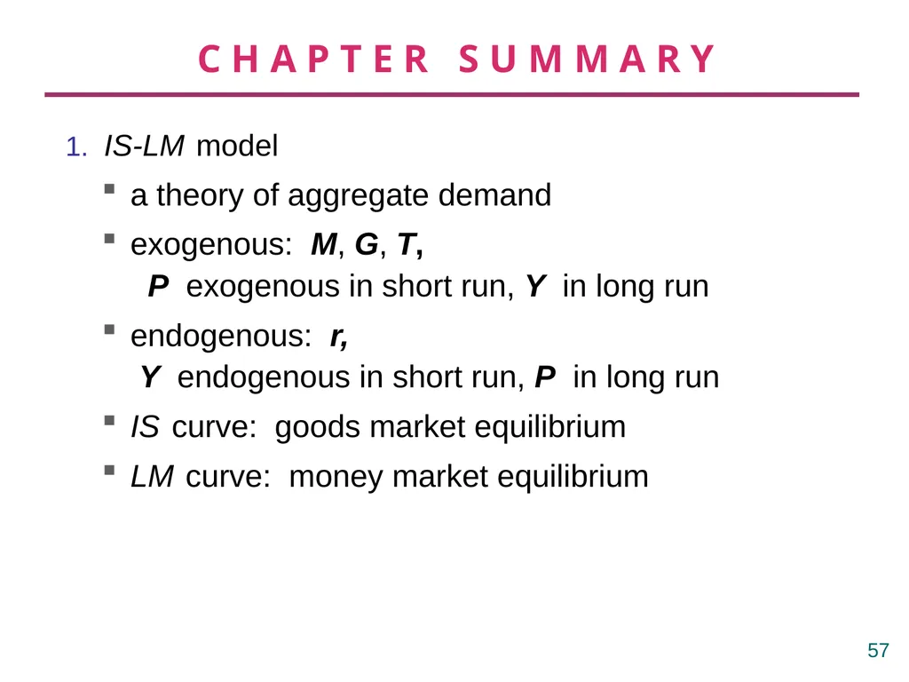
slide57. CHAPTER SUMMARY 1. IS-LM model
a theory of aggregate demand
exogenous: M, G, T, P exogenous in short run, Y in long run
endogenous: r, Y endogenous in short run, P in long run
IS curve: goods market equilibrium
LM curve: money market equilibrium 56<br>
slide58. CHAPTER SUMMARY 2. AD curve
shows relation between P and the IS-LM model’s equilibrium Y.
negative slope because hP g i(M/P) g hr g iI g iY
expansionary fiscal policy shifts IS curve right, raises income, and shifts AD curve right.
expansionary monetary policy shifts LM curve right, raises income, and shifts AD curve right.
IS or LM shocks shift the AD curve. 57<br>