Analyzing large-scale achievement surveys in Stata using PISATOOLS and PIAACTOOLS Dr Maciej Jakubowski Evidence Institute and Warsaw University November 2017 Agenda for today What are large-scale achievement surveys? Complex survey
"Analyzing large-scale achievement surveys in Stata" is the property of its rightful owner. Permission is granted to
download and print the materials on this website for personal, non-commercial use only, and to display it
on your personal computer provided you do not modify the materials and that you retain all copyright
notices contained in the materials. By downloading content from our website, you accept the terms of this
agreement.
Presentation Transcript
01
Analyzing large-scale achievement surveys in Stata using
PISATOOLS and PIAACTOOLS
Dr Maciej Jakubowski
Evidence Institute and Warsaw University November 2017<br>
02
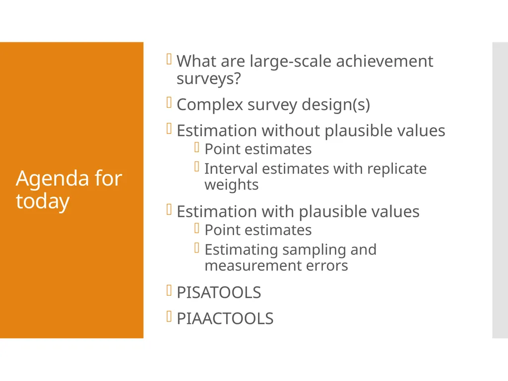
Agenda for today What are large-scale achievement surveys?
Complex survey design(s)
Estimation without plausible values
Point estimates
Interval estimates with replicate weights
Estimation with plausible values
Point estimates
Estimating sampling and measurement errors
PISATOOLS
PIAACTOOLS<br>
03
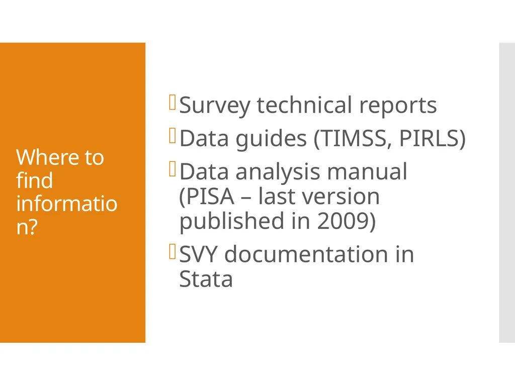
Where to find information? Survey technical reports
Data guides (TIMSS, PIRLS)
Data analysis manual (PISA – last version published in 2009)
SVY documentation in Stata<br>
04
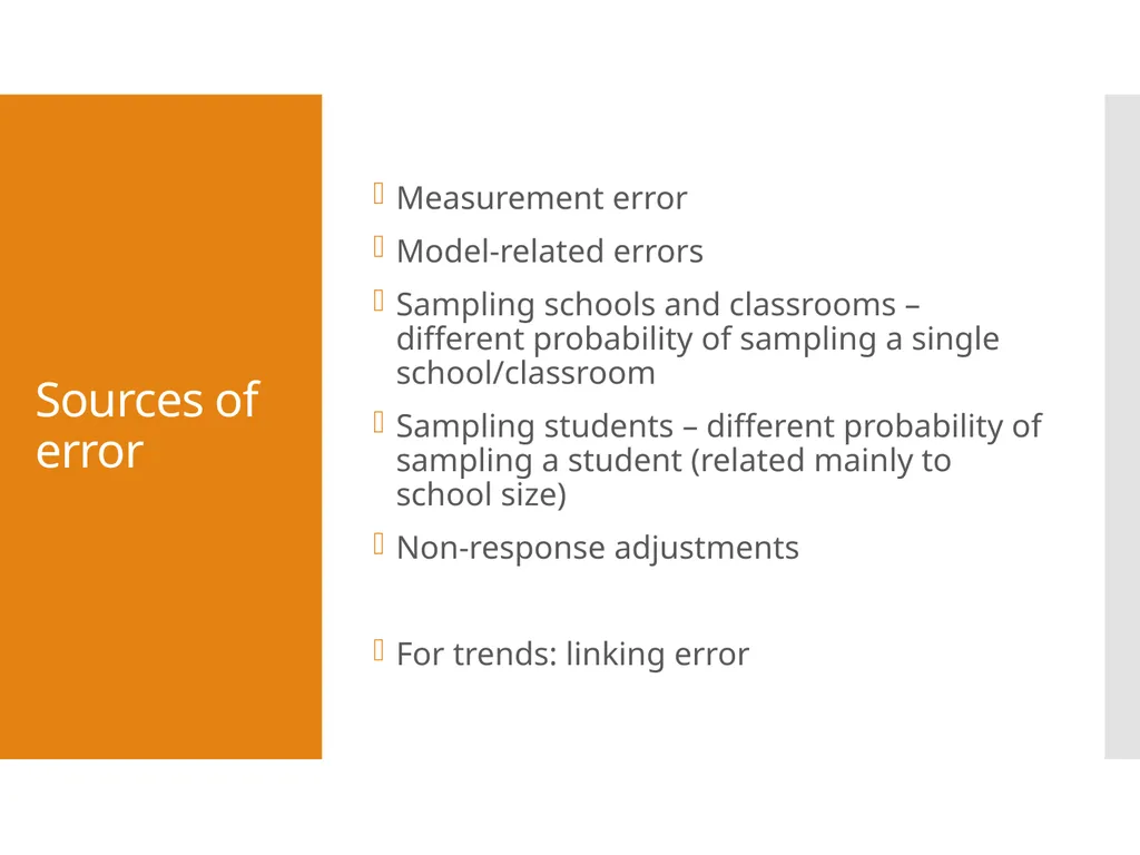
Sources of error Measurement error
Model-related errors
Sampling schools and classrooms – different probability of sampling a single school/classroom
Sampling students – different probability of sampling a student (related mainly to school size)
Non-response adjustments
For trends: linking error<br>
05
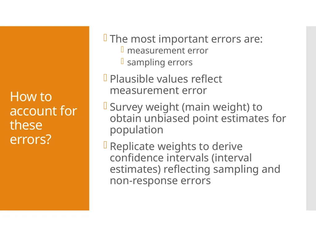
How to account for these errors? The most important errors are:
measurement error
sampling errors
Plausible values reflect measurement error
Survey weight (main weight) to obtain unbiased point estimates for population
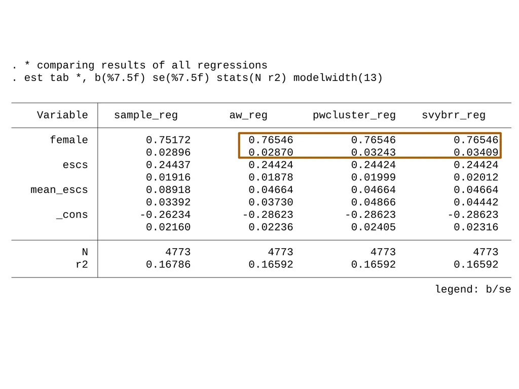
Replicate weights to derive confidence intervals (interval estimates) reflecting sampling and non-response errors<br>
06
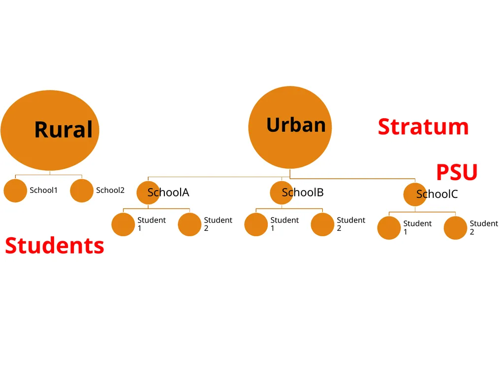
Survey weights Stratum PSU Students<br>
07
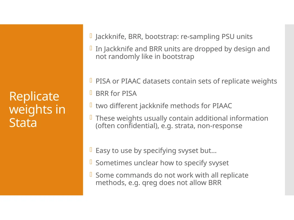
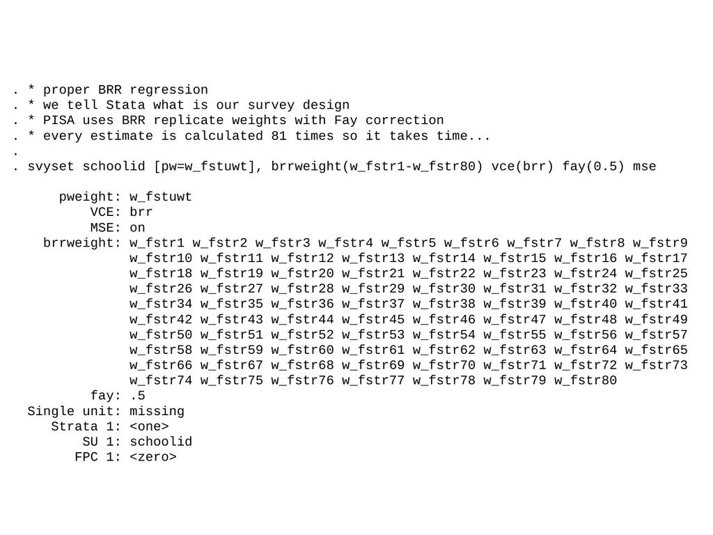
Replicate weights in Stata Jackknife, BRR, bootstrap: re-sampling PSU units
In Jackknife and BRR units are dropped by design and not randomly like in bootstrap
PISA or PIAAC datasets contain sets of replicate weights
BRR for PISA
two different jackknife methods for PIAAC
These weights usually contain additional information (often confidential), e.g. strata, non-response
Easy to use by specifying svyset but…
Sometimes unclear how to specify svyset
Some commands do not work with all replicate methods, e.g. qreg does not allow BRR<br>
08
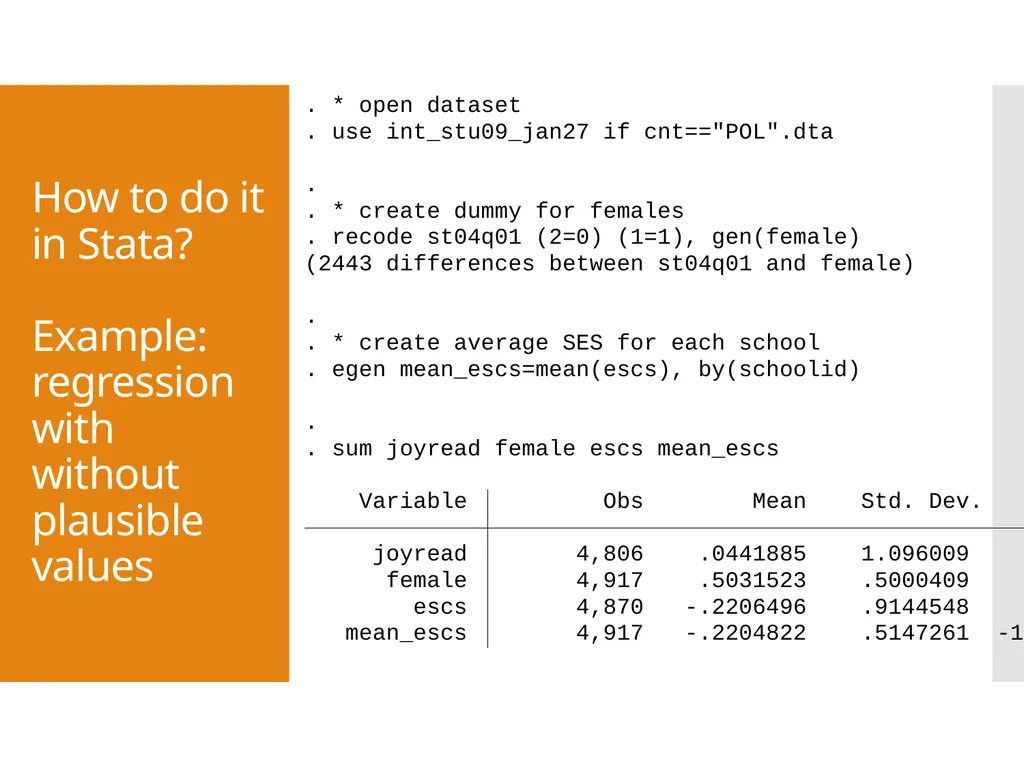
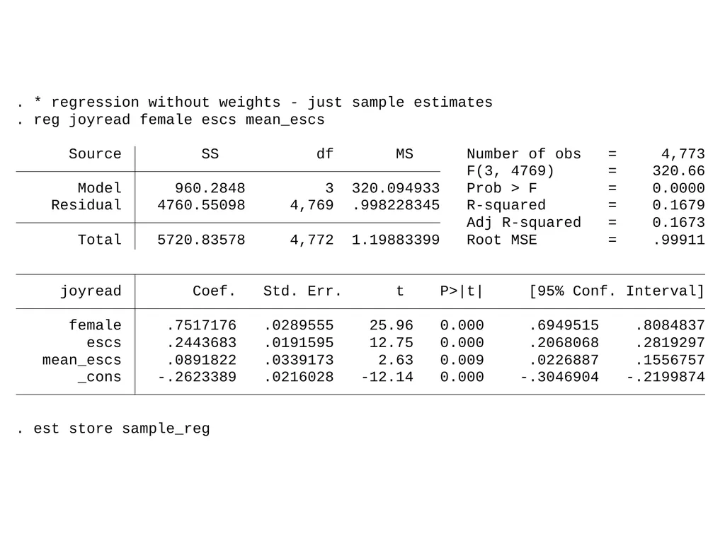
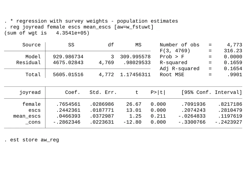
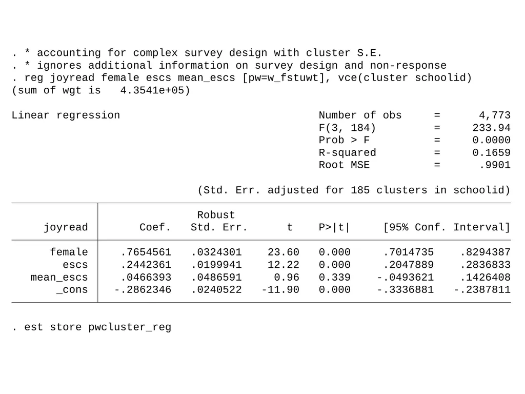
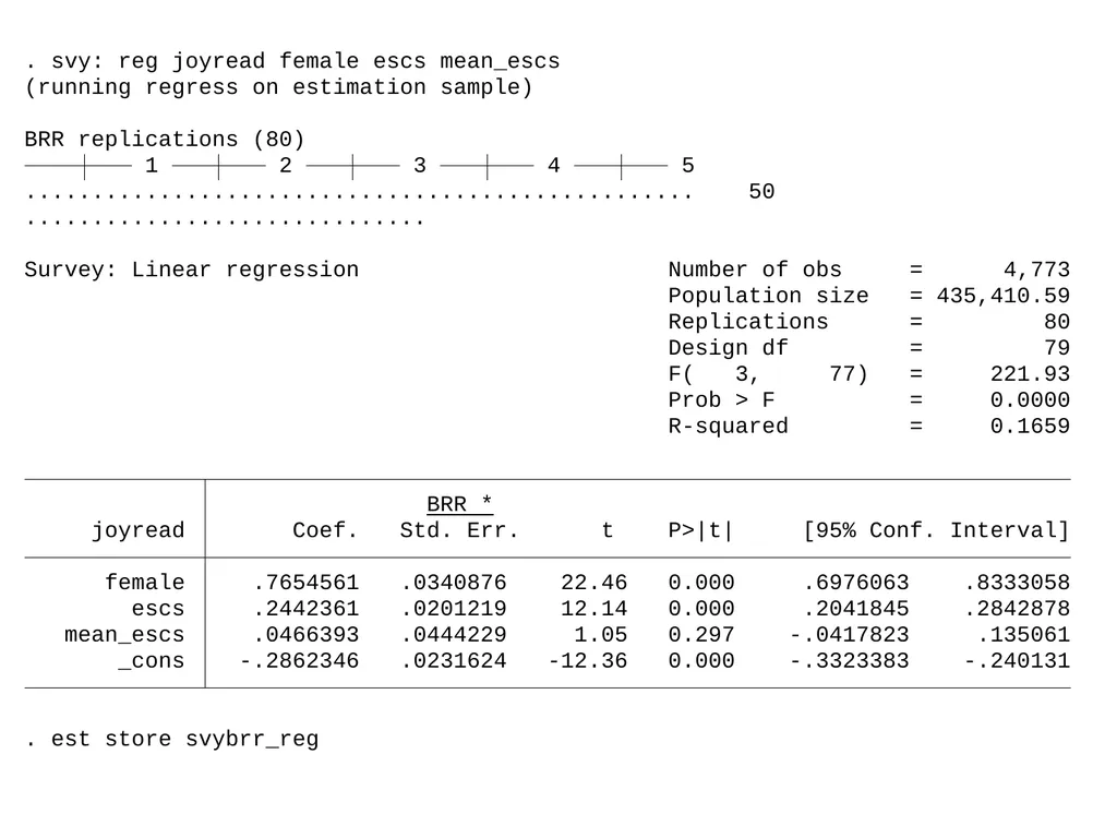
How to do it in Stata? Example: regression with without plausible values<br>
09
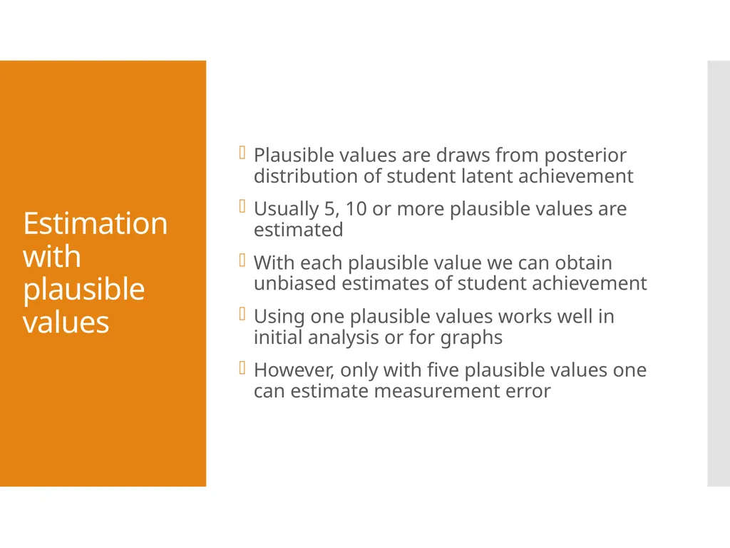
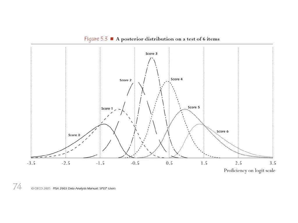
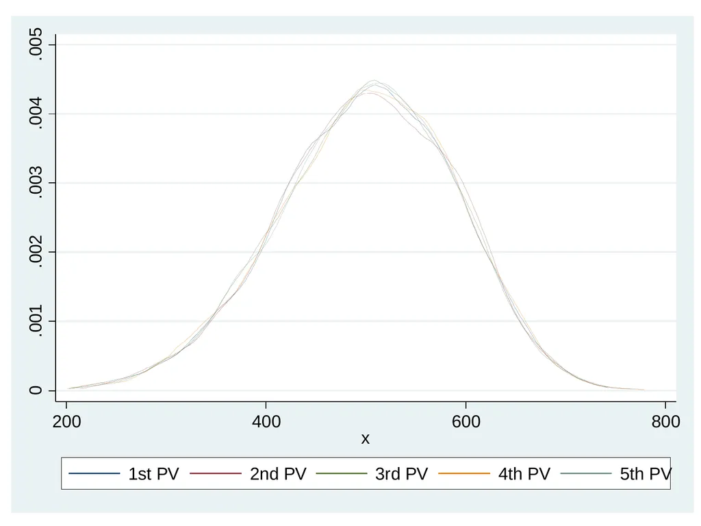
Estimation with plausible values Plausible values are draws from posterior distribution of student latent achievement
Usually 5, 10 or more plausible values are estimated
With each plausible value we can obtain unbiased estimates of student achievement
Using one plausible values works well in initial analysis or for graphs
However, only with five plausible values one can estimate measurement error<br>
10
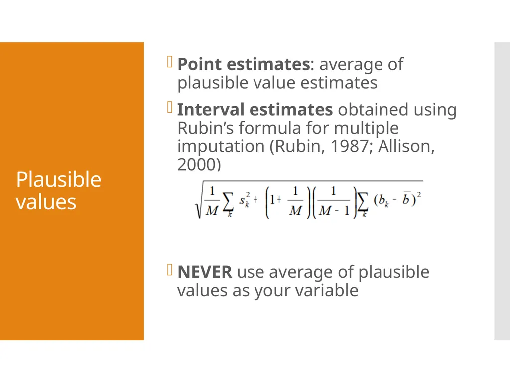
Plausible values Point estimates: average of plausible value estimates
Interval estimates obtained using Rubin’s formula for multiple imputation (Rubin, 1987; Allison, 2000)
NEVER use average of plausible values as your variable<br>
11
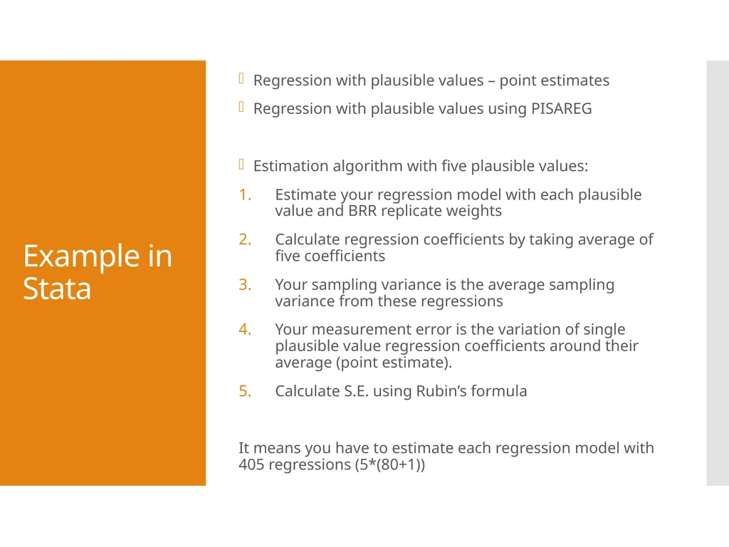
Example in Stata Regression with plausible values – point estimates
Regression with plausible values using PISAREG
Estimation algorithm with five plausible values:
Estimate your regression model with each plausible value and BRR replicate weights
Calculate regression coefficients by taking average of five coefficients
Your sampling variance is the average sampling variance from these regressions
Your measurement error is the variation of single plausible value regression coefficients around their average (point estimate).
Calculate S.E. using Rubin’s formula
It means you have to estimate each regression model with 405 regressions (5*(80+1))<br>
12
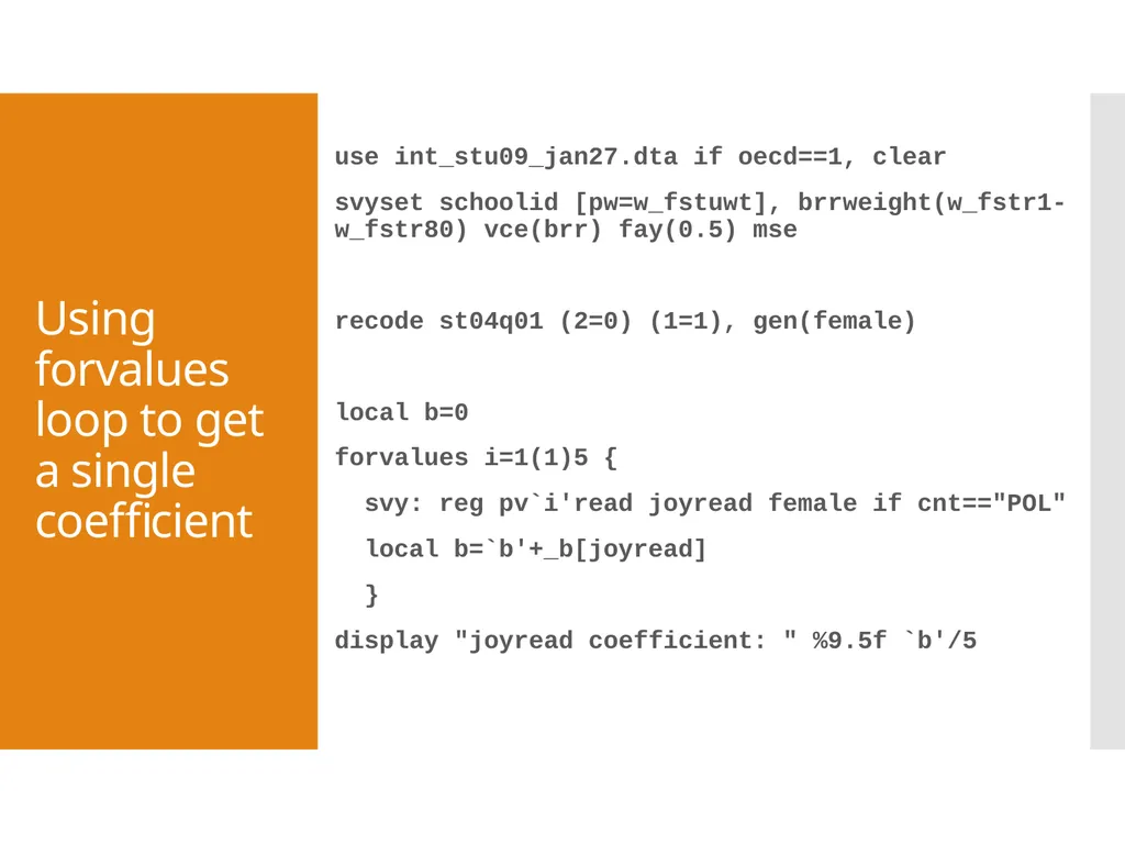
Using forvalues loop to get a single coefficient use int_stu09_jan27.dta if oecd==1, clear
svyset schoolid [pw=w_fstuwt], brrweight(w_fstr1-w_fstr80) vce(brr) fay(0.5) mse
recode st04q01 (2=0) (1=1), gen(female)
local b=0
forvalues i=1(1)5 {
svy: reg pv`i'read joyread female if cnt=="POL"
local b=`b'+_b[joyread]
}
display "joyread coefficient: " %9.5f `b'/5<br>
13
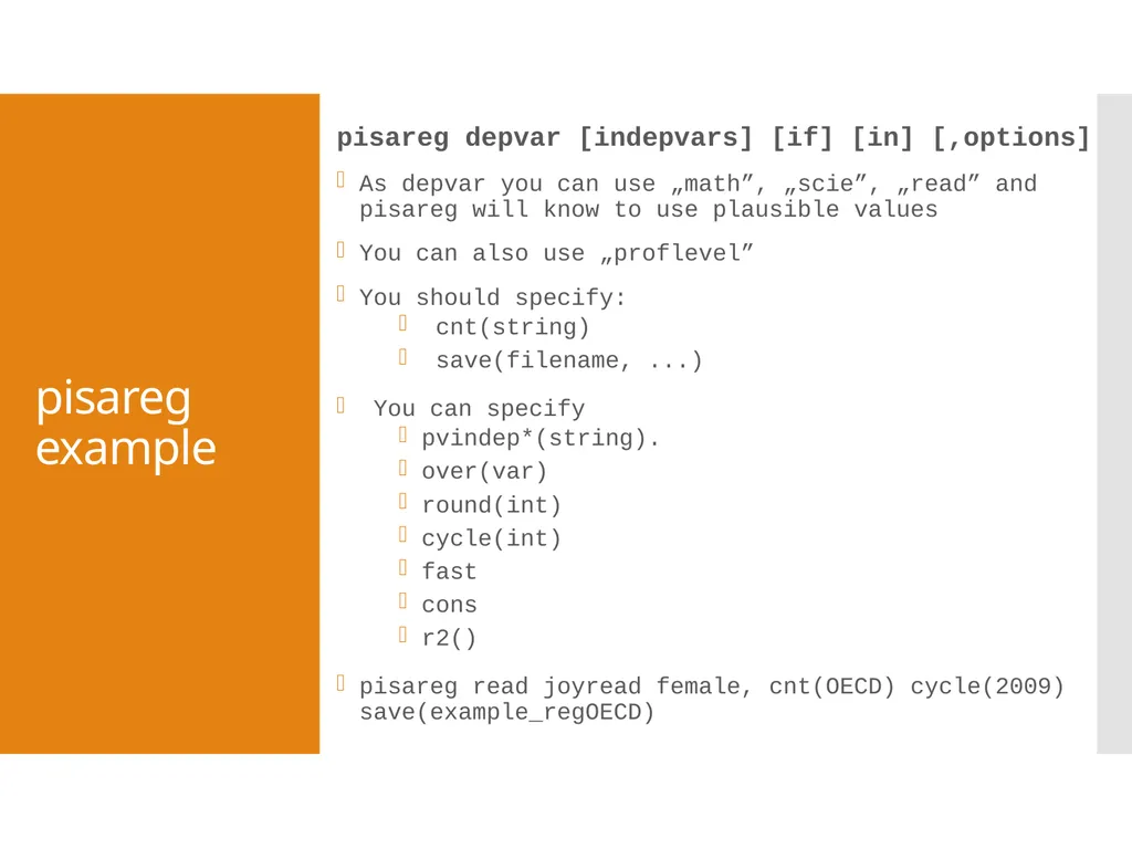
pisareg example pisareg depvar [indepvars] [if] [in] [,options]
As depvar you can use „math”, „scie”, „read” and pisareg will know to use plausible values
You can also use „proflevel”
You should specify:
cnt(string)
save(filename, ...)
You can specify
pvindep*(string).
over(var)
round(int)
cycle(int)
fast
cons
r2()
pisareg read joyread female, cnt(OECD) cycle(2009) save(example_regOECD)<br>
14
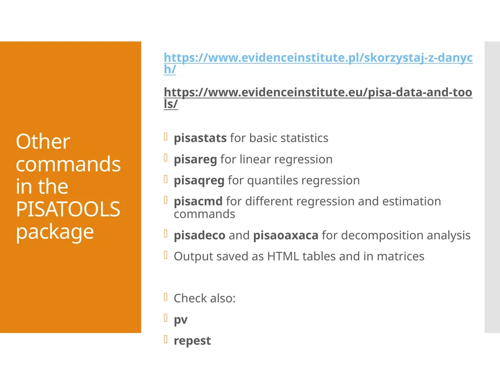
Other commands in the PISATOOLS package https://www.evidenceinstitute.pl/skorzystaj-z-danych/
https://www.evidenceinstitute.eu/pisa-data-and-tools/
pisastats for basic statistics
pisareg for linear regression
pisaqreg for quantiles regression
pisacmd for different regression and estimation commands
pisadeco and pisaoaxaca for decomposition analysis
Output saved as HTML tables and in matrices
Check also:
pv
repest<br>
15
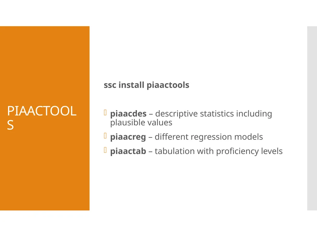
PIAACTOOLS ssc install piaactools
piaacdes – descriptive statistics including plausible values
piaacreg – different regression models
piaactab – tabulation with proficiency levels<br>
16
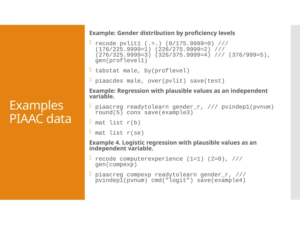
Examples PIAAC data Example: Gender distribution by proficiency levels
recode pvlit1 (.=.) (0/175.9999=0) /// (176/225.9999=1) (226/275.9999=2) /// (276/325.9999=3) (326/375.9999=4) /// (376/999=5), gen(proflevel1)
tabstat male, by(proflevel)
piaacdes male, over(pvlit) save(test)
Example: Regression with plausible values as an independent variable.
piaacreg readytolearn gender_r, /// pvindep1(pvnum) round(5) cons save(example3)
mat list r(b)
mat list r(se)
Example 4. Logistic regression with plausible values as an independent variable.
recode computerexperience (1=1) (2=0), /// gen(compexp)
piaacreg compexp readytolearn gender_r, /// pvindep1(pvnum) cmd("logit") save(example4)<br>
17
Zapraszamy do kontaktu! mj@evidenceinstitute.pl
www.facebook.com/EvidenceInstitutePL
@JakubowskiEvid
www.evidenceinstitute.pl<br>