
Bayesian data analysis: What is it and when should
PC
Published · 30 slides · 0 views
1 / 1
Description
Bayesian data analysis: What is it and when should you care? First, whatwho is Bayes? The Reverend Thomas Bayes was an English statistician, philosopher, and minister He developed Bayes theorem to integrate prior probabilities with new
Related Topics
Share
Embed code
Download this presentation From Below
"Bayesian data analysis: What is it and when should" is the property of its rightful owner. Permission is granted to download and print the materials on this website for personal, non-commercial use only, and to display it on your personal computer provided you do not modify the materials and that you retain all copyright notices contained in the materials. By downloading content from our website, you accept the terms of this agreement.
Presentation Transcript
01
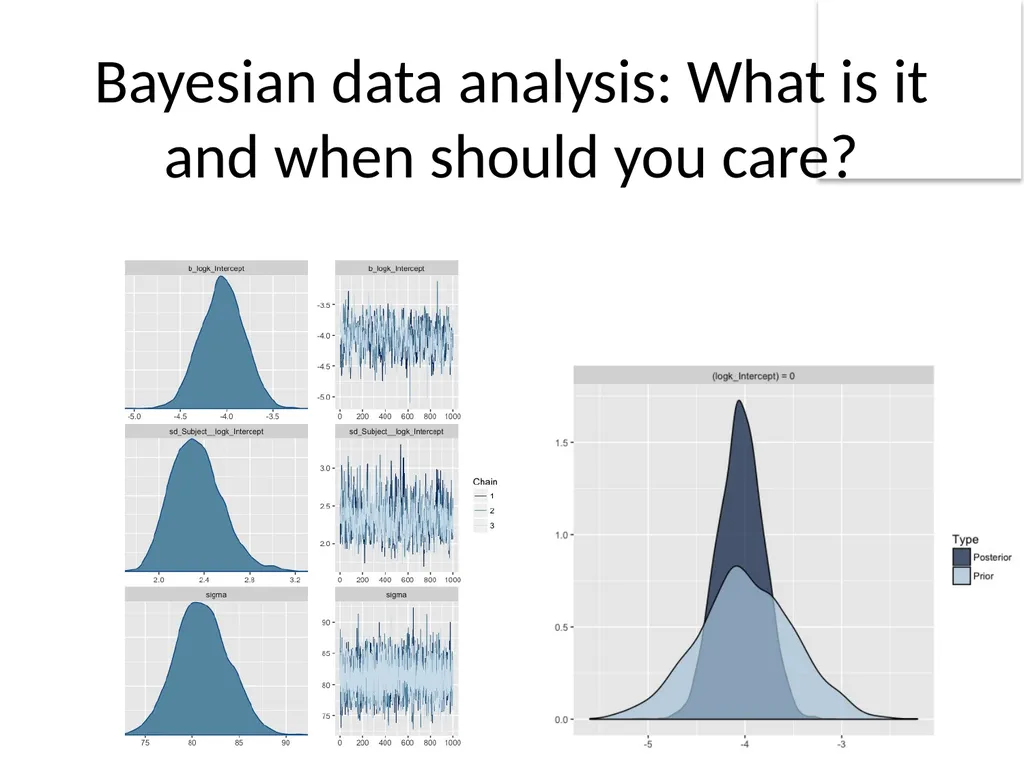
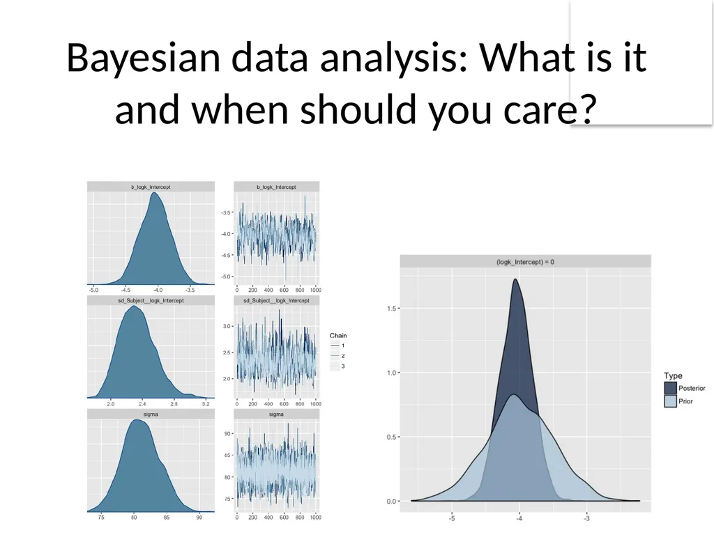
Bayesian data analysis: What is it and when should you care?<br>
02
First, what/who is Bayes? The Reverend Thomas Bayes was an English statistician, philosopher, and minister
He developed Bayes’ theorem to integrate prior probabilities with new evidence to calculate a posterior probabilities
P(guilty | evidence) is based on P(guilty) before evidence is collected and the P(evidence | guilty)<br>
He developed Bayes’ theorem to integrate prior probabilities with new evidence to calculate a posterior probabilities
P(guilty | evidence) is based on P(guilty) before evidence is collected and the P(evidence | guilty)<br>
03
Bayes’ theorem and statistics Traditional statistical methods find P(data | hypothesis) – most commonly, P(D|H0)
But, Bayesians point out that what we think we are calculating is P(H0|D) – but we’re not!
The probability of any particular point estimate of a parameter is TINY and thus meaningless in isolation
To appreciate the difference between the two Ps
P(coin flip came up tails | two-tailed coin) vs.
P(two-tailed coin | coin flip came up tails )? P(H2-tailed|D) P(D|H2-tailed)<br>
But, Bayesians point out that what we think we are calculating is P(H0|D) – but we’re not!
The probability of any particular point estimate of a parameter is TINY and thus meaningless in isolation
To appreciate the difference between the two Ps
P(coin flip came up tails | two-tailed coin) vs.
P(two-tailed coin | coin flip came up tails )? P(H2-tailed|D) P(D|H2-tailed)<br>
04
Bayesian statistics If we want to know, P(Hx|D), we need to know P(D|Hx) and P(Hx)
P(Hx) = prior probability of hypothesis x
Before we collect the data/evidence
P(Hx|D) = posterior probability of hypothesis x
After we collect the data/evidence
Given that these posterior probabilities are TINY, what is useful is to compare these probabilities: P(Hm=5|D)/P(Hm=0|D)
This is a Bayes Factor or relatively likelihood in favor of one hypothesis vs. another
For this example, if the ratio/BF is 1, then equally likely that mean is 0 or 5. If ratio > 1, then more likely it’s 5; if ratio < 1 then more likely it’s 0.<br>
P(Hx) = prior probability of hypothesis x
Before we collect the data/evidence
P(Hx|D) = posterior probability of hypothesis x
After we collect the data/evidence
Given that these posterior probabilities are TINY, what is useful is to compare these probabilities: P(Hm=5|D)/P(Hm=0|D)
This is a Bayes Factor or relatively likelihood in favor of one hypothesis vs. another
For this example, if the ratio/BF is 1, then equally likely that mean is 0 or 5. If ratio > 1, then more likely it’s 5; if ratio < 1 then more likely it’s 0.<br>
05
Two ways Bayesians are influencing current analysis of data Bayes factors
This is a metric used for model comparison as in earlier example
Bayesian data analysis
This incorporates “prior distributions” or “priors” about parameters and updates them with data from your study to produce a “posterior distribution” for the parameter<br>
This is a metric used for model comparison as in earlier example
Bayesian data analysis
This incorporates “prior distributions” or “priors” about parameters and updates them with data from your study to produce a “posterior distribution” for the parameter<br>
06
Bayes factor You proceed to run analyses as you normally do
Either you have two explicit models (e.g., A+B vs. A+B+A*B), or
You have one model where the alternative is implied as the null model
The BF is designed to provide a measure of “evidence” in favor of one model over the other
This is a likelihood ratio based on BIC values to adjust for model complexity, e.g., BF01 = exp(DBIC10/2)<br>
Either you have two explicit models (e.g., A+B vs. A+B+A*B), or
You have one model where the alternative is implied as the null model
The BF is designed to provide a measure of “evidence” in favor of one model over the other
This is a likelihood ratio based on BIC values to adjust for model complexity, e.g., BF01 = exp(DBIC10/2)<br>
07
Bayesian data analysis Bayesian data analysis goes full-bore – the analysis is entirely different
You begin by specifying prior distributions for each parameter in a model
Regression weights (bi), sd of each bi, residual sd, correlations between measures, sd of random effect estimates, etc.
You integrate the data (i.e., new evidence)
Computer considers a specific parameter estimate, it computes the likelihood of observing your data for this estimate, and finally combines this likelihood with the prior probability of this estimate to get P(Hestimate | D)
Then system chooses another parameter estimate and computes the posterior probability again…
And then again, and again, and again…
Oh, and it has to do this for multiple parameters at the same time…
Can you say “computationally expensive?”
Finally, you end up with a posterior distribution of each parameter<br>
You begin by specifying prior distributions for each parameter in a model
Regression weights (bi), sd of each bi, residual sd, correlations between measures, sd of random effect estimates, etc.
You integrate the data (i.e., new evidence)
Computer considers a specific parameter estimate, it computes the likelihood of observing your data for this estimate, and finally combines this likelihood with the prior probability of this estimate to get P(Hestimate | D)
Then system chooses another parameter estimate and computes the posterior probability again…
And then again, and again, and again…
Oh, and it has to do this for multiple parameters at the same time…
Can you say “computationally expensive?”
Finally, you end up with a posterior distribution of each parameter<br>
08
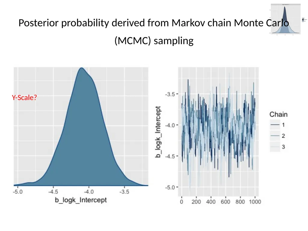
Posterior probability derived from Markov chain Monte Carlo (MCMC) sampling Y-Scale?<br>
09
Empirically-derived parameter distributions Thus, Bayesian data analysis assumes much less about your data
Rather, it estimates the likelihood of each value of a parameter
This allows statements about relative likelihood<br>
Rather, it estimates the likelihood of each value of a parameter
This allows statements about relative likelihood<br>
10
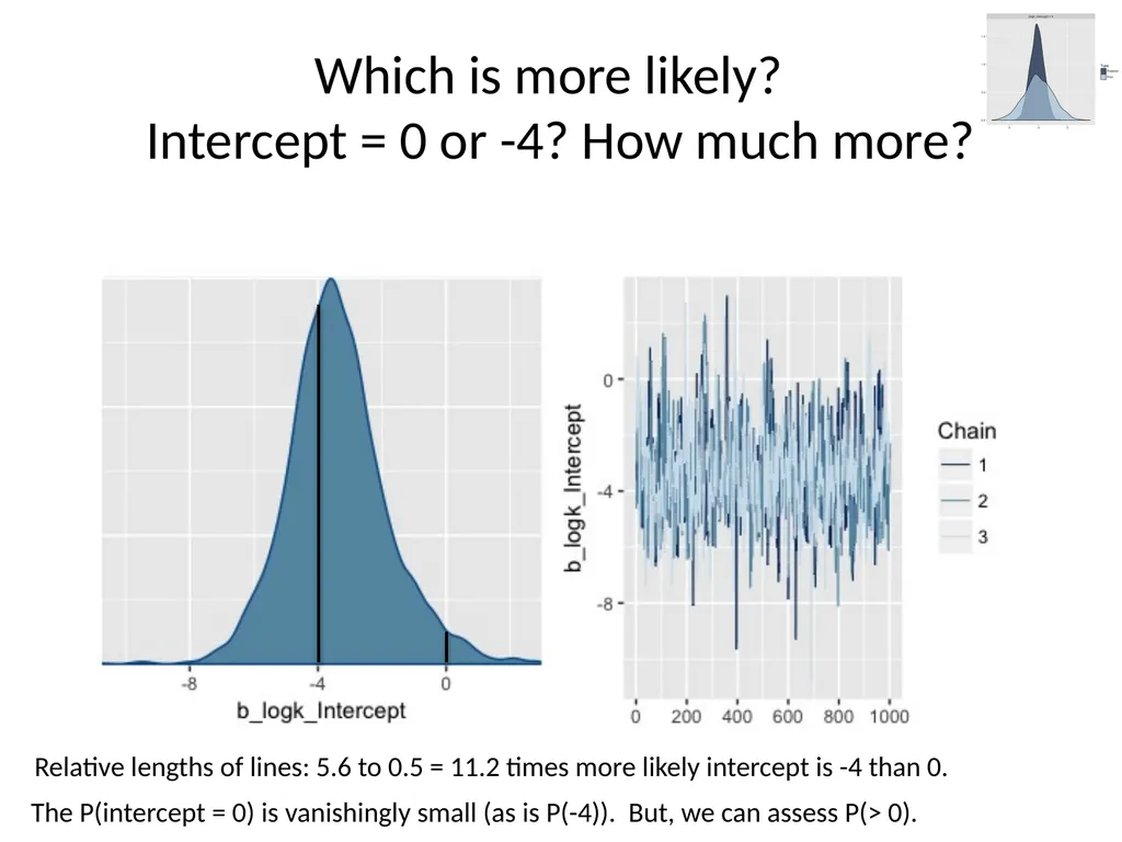
Which is more likely?
Intercept = 0 or -4? How much more? Relative lengths of lines: 5.6 to 0.5 = 11.2 times more likely intercept is -4 than 0. The P(intercept = 0) is vanishingly small (as is P(-4)). But, we can assess P(> 0).<br>
11
Priors Most Bayesian analysts assume “uninformative priors”
no strong assumptions about the parameter estimates other than the shape of their distributions
In my experience, when you use uninformative priors and analyze the data using both a traditional approach and a Bayesian approach, the resulting parameter estimates are the same (for all practical purposes) = no strong rationale for Bayesian
Uninformative priors means the results are strongly determined by the current experiment’s data<br>
no strong assumptions about the parameter estimates other than the shape of their distributions
In my experience, when you use uninformative priors and analyze the data using both a traditional approach and a Bayesian approach, the resulting parameter estimates are the same (for all practical purposes) = no strong rationale for Bayesian
Uninformative priors means the results are strongly determined by the current experiment’s data<br>
12
When should I consider Bayesian analysis? When you are willing to specify informative priors
When there is no existing analysis for your design<br>
When there is no existing analysis for your design<br>
13
Informative priors One non-controversial way to specify priors is to indicate their shape and/or limits
For example, if k is typically skewed with a minimum of zero, then you can specify an appropriate distribution class for k (like the Gamma)
A more controversial way to specify a prior is to suggest a narrower range around a particular value
If current data set is small or highly variable, resulting estimates will be strongly determined by the priors with a minor update<br>
For example, if k is typically skewed with a minimum of zero, then you can specify an appropriate distribution class for k (like the Gamma)
A more controversial way to specify a prior is to suggest a narrower range around a particular value
If current data set is small or highly variable, resulting estimates will be strongly determined by the priors with a minor update<br>
14
How to ethically specify narrower priors If you are conducting an experiment (or condition) that is a direct replication of an earlier study
Can use parameter estimate from earlier study along with its SE
“Today’s posterior is tomorrow’s prior”
NOTE: cannot just use part of your data to establish a prior and then analyze full data set based on this prior – prior = independent data
If you are conducting an experiment very similar to earlier studies, then choose an estimated value consistent with that observed before, but increase your SD to encompass all prior estimates
E.g., prior estimates are 4 ± 2, 3 ± 1, 5 ± 5, then use something like 4 ± 6 (where 2nd number is SE)
Better yet, if there is a meta-analysis that’s been conducted, use the mean effect size and its 95% CI from the literature
Can also limit prior specification to parameters that do not involve the treatment effect (e.g., intercept or random effect s.d.)<br>
Can use parameter estimate from earlier study along with its SE
“Today’s posterior is tomorrow’s prior”
NOTE: cannot just use part of your data to establish a prior and then analyze full data set based on this prior – prior = independent data
If you are conducting an experiment very similar to earlier studies, then choose an estimated value consistent with that observed before, but increase your SD to encompass all prior estimates
E.g., prior estimates are 4 ± 2, 3 ± 1, 5 ± 5, then use something like 4 ± 6 (where 2nd number is SE)
Better yet, if there is a meta-analysis that’s been conducted, use the mean effect size and its 95% CI from the literature
Can also limit prior specification to parameters that do not involve the treatment effect (e.g., intercept or random effect s.d.)<br>
15
The goal – incremental science! This approach moves psychology from a bunch of individual studies that are occasionally combined using meta-analysis to one that approaches the best estimate for parameters by having earlier studies inform the current one<br>
16
The effect of priors… Narrower priors will have a bigger effect on the posterior estimation
The effect will be larger if the new data is limited or highly variable
This situation indicates that the new data are equivocal and offer little new<br>
The effect will be larger if the new data is limited or highly variable
This situation indicates that the new data are equivocal and offer little new<br>
17
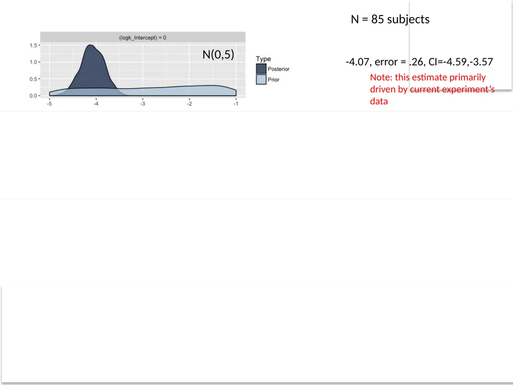
-4.07, error = .26, CI=-4.59,-3.57 -4.05, error = .24, CI=-4.52,-3.59 -4.03, error = .18, CI=-4.37,-3.67 -2.86, error = .21, CI=-3.28,-2.45 N(0,5) N(-4,.5) N(-4,.25) N(-2,.25) N = 85 subjects Note: uncertainty in prior and data are similar so estimate in middle Note: this estimate primarily driven by current experiment’s data<br>
18
N = 20 with same priors? -3.62, error = .73, CI = -5.08,-2.09 - N(0, 5)
-3.88, error = .40, CI = -4.68,-3.10 - N(-4, .5)
-3.97, error = .23, CI = -4.42,-3.52 - N(-4, .25)
-2.17, error = .24, CI = -2.65,-1.70 - N(-2, .25)
With narrow priors and small sample, result is strongly driven by prior
Current experiment has broad CI (-5.08,-2.09) which encompasses the updated estimate in all four cases<br>
-3.88, error = .40, CI = -4.68,-3.10 - N(-4, .5)
-3.97, error = .23, CI = -4.42,-3.52 - N(-4, .25)
-2.17, error = .24, CI = -2.65,-1.70 - N(-2, .25)
With narrow priors and small sample, result is strongly driven by prior
Current experiment has broad CI (-5.08,-2.09) which encompasses the updated estimate in all four cases<br>
19
When should you care?
(i.e., when to consider Bayesian?) When you have earlier evidence on which to base a prior
Creates a more powerful result and incremental science
When you want to limit the range of parameter estimates or their distributions to something “realistic”
When standard models aren’t available
Multilevel multinomial logistic regression
Multilevel models with non-standard distributions (e.g., due to censoring)
Nonlinear models with non-normal error distributions<br>
Creates a more powerful result and incremental science
When you want to limit the range of parameter estimates or their distributions to something “realistic”
When standard models aren’t available
Multilevel multinomial logistic regression
Multilevel models with non-standard distributions (e.g., due to censoring)
Nonlinear models with non-normal error distributions<br>
20
Example: Doing the previously impossible Tony’s experiment involves measuring latencies to respond on the BART
On many trials, the trial ends before a response was made, so all we know is that the person waited longer than that time
How to handle this?
Conventional approaches – substitute latency as the max time for these trials; treat these latencies as missing values; perhaps supplement these analyses by independently analyzing the likelihood of not responding
Modern approach – these are ‘censored’ trials
Problem – not able to do repeated measures censored regression<br>
On many trials, the trial ends before a response was made, so all we know is that the person waited longer than that time
How to handle this?
Conventional approaches – substitute latency as the max time for these trials; treat these latencies as missing values; perhaps supplement these analyses by independently analyzing the likelihood of not responding
Modern approach – these are ‘censored’ trials
Problem – not able to do repeated measures censored regression<br>
21
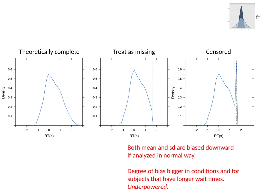
Theoretically complete Treat as missing Censored Both mean and sd are biased downward
If analyzed in normal way.
Degree of bias bigger in conditions and for subjects that have longer wait times. Underpowered.<br>
If analyzed in normal way.
Degree of bias bigger in conditions and for subjects that have longer wait times. Underpowered.<br>
22
Tony’s project Tony tried a method to prevent censoring by letting them respond until end of trial and giving them feedback that the trial ended prematurely AFTER the trial ended
Two conditions:
Inflate to pop (standard) and Inflate to full (new)
Implications? Did we introduce any fundamental change in behavior by delaying feedback?
Recent reanalysis using censored regression<br>
Two conditions:
Inflate to pop (standard) and Inflate to full (new)
Implications? Did we introduce any fundamental change in behavior by delaying feedback?
Recent reanalysis using censored regression<br>
23
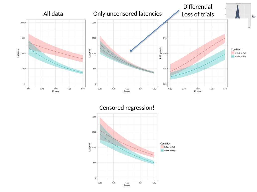
All data Only uncensored latencies Differential
Loss of trials Censored regression!<br>
Loss of trials Censored regression!<br>
24
Censoring is common in certain
animal experiments Trial terminates before subject responds
For example, Morris water maze: rat removed from water if it doesn’t find platform within 90 s
If censored trials excluded, estimates are biased downward
If censored trials treated as maximum but analyzed normally…
estimates still biased downward but less strongly,
creates bimodal error distribution which violates normality assumption<br>
For example, Morris water maze: rat removed from water if it doesn’t find platform within 90 s
If censored trials excluded, estimates are biased downward
If censored trials treated as maximum but analyzed normally…
estimates still biased downward but less strongly,
creates bimodal error distribution which violates normality assumption<br>
25
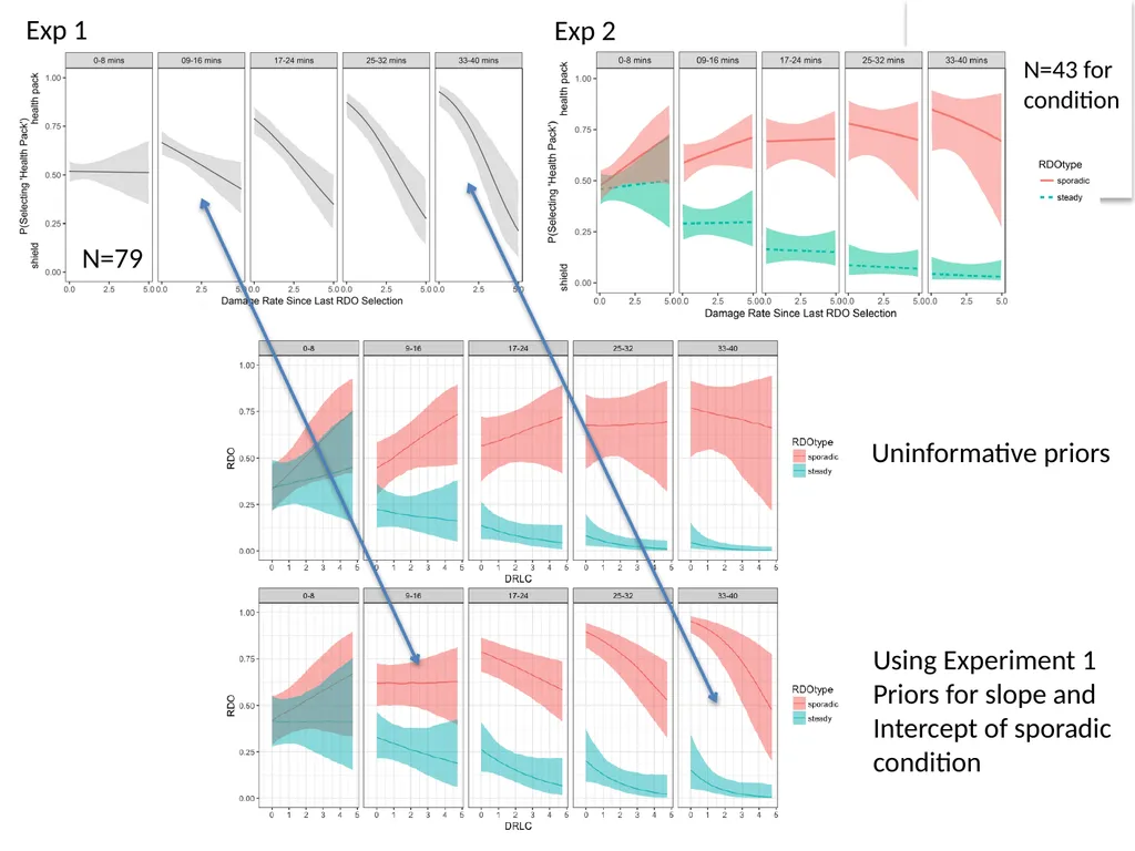
Example: specifying priors Lisa ran two experiments for her Masters thesis
Experiment 1 involved the relative use of two risk mitigation strategies (shield vs. health pack)
The shield was available only for a short time after being activated
Experiment 2 had two conditions
Sporadic – same as Experiment 1
Steady – new condition in which shield available until used
The sporadic condition of Experiment 2 was a replication but had about half the subjects of Experiment 1<br>
Experiment 1 involved the relative use of two risk mitigation strategies (shield vs. health pack)
The shield was available only for a short time after being activated
Experiment 2 had two conditions
Sporadic – same as Experiment 1
Steady – new condition in which shield available until used
The sporadic condition of Experiment 2 was a replication but had about half the subjects of Experiment 1<br>
26
Uninformative priors Using Experiment 1
Priors for slope and
Intercept of sporadic
condition N=79 N=43 for condition Exp 1 Exp 2<br>
Priors for slope and
Intercept of sporadic
condition N=79 N=43 for condition Exp 1 Exp 2<br>
27
Take home message Bayesian analysis can allow you to do new things that better model the processes under study
Multilevel censored regression
Multilevel multinomial logistic regression (e.g., ordinal)
Nonlinear multilevel models with non-normal error distributions (e.g., hyperbolic functions!)
Robust linear models
Specification of Weibull, Ex-Gaussian, Beta, negative binomial… 29 different y distributions!
Bayesian analysis encourages incremental science in which we build on prior results
Rewards direct replications by making prior distribution specification straightforward<br>
Multilevel censored regression
Multilevel multinomial logistic regression (e.g., ordinal)
Nonlinear multilevel models with non-normal error distributions (e.g., hyperbolic functions!)
Robust linear models
Specification of Weibull, Ex-Gaussian, Beta, negative binomial… 29 different y distributions!
Bayesian analysis encourages incremental science in which we build on prior results
Rewards direct replications by making prior distribution specification straightforward<br>
28
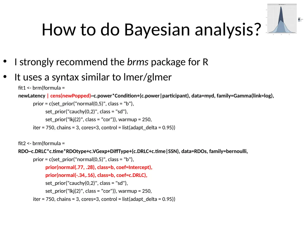
How to do Bayesian analysis? I strongly recommend the brms package for R
It uses a syntax similar to lmer/glmer
fit1 <- brm(formula =
newLatency | cens(newPopped)~c.power*Condition+(c.power|participant), data=myd, family=Gamma(link=log),
prior = c(set_prior("normal(0,5)", class = "b"),
set_prior("cauchy(0,2)", class = "sd"),
set_prior("lkj(2)", class = "cor")), warmup = 250,
iter = 750, chains = 3, cores=3, control = list(adapt_delta = 0.95))
fit2 <- brm(formula =
RDO~c.DRLC*c.time*RDOtype+c.VGexp+DiffType+(c.DRLC+c.time|SSN), data=RDOs, family=bernoulli,
prior = c(set_prior("normal(0,5)", class = "b"),
prior(normal(.77, .28), class=b, coef=Intercept),
prior(normal(-.34,.16), class=b, coef=c.DRLC),
set_prior("cauchy(0,2)", class = "sd"),
set_prior("lkj(2)", class = "cor")), warmup = 250,
iter = 750, chains = 3, cores=3, control = list(adapt_delta = 0.95))<br>
It uses a syntax similar to lmer/glmer
fit1 <- brm(formula =
newLatency | cens(newPopped)~c.power*Condition+(c.power|participant), data=myd, family=Gamma(link=log),
prior = c(set_prior("normal(0,5)", class = "b"),
set_prior("cauchy(0,2)", class = "sd"),
set_prior("lkj(2)", class = "cor")), warmup = 250,
iter = 750, chains = 3, cores=3, control = list(adapt_delta = 0.95))
fit2 <- brm(formula =
RDO~c.DRLC*c.time*RDOtype+c.VGexp+DiffType+(c.DRLC+c.time|SSN), data=RDOs, family=bernoulli,
prior = c(set_prior("normal(0,5)", class = "b"),
prior(normal(.77, .28), class=b, coef=Intercept),
prior(normal(-.34,.16), class=b, coef=c.DRLC),
set_prior("cauchy(0,2)", class = "sd"),
set_prior("lkj(2)", class = "cor")), warmup = 250,
iter = 750, chains = 3, cores=3, control = list(adapt_delta = 0.95))<br>
29
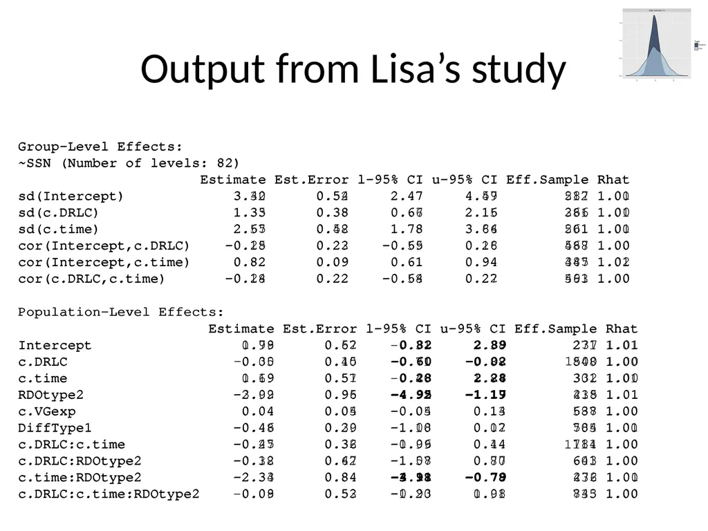
Output from Lisa’s study Group-Level Effects:
~SSN (Number of levels: 82)
Estimate Est.Error l-95% CI u-95% CI Eff.Sample Rhat
sd(Intercept) 3.40 0.54 2.47 4.57 287 1.01
sd(c.DRLC) 1.35 0.38 0.67 2.16 266 1.00
sd(c.time) 2.65 0.52 1.78 3.84 261 1.01
cor(Intercept,c.DRLC) -0.25 0.22 -0.65 0.18 567 1.00
cor(Intercept,c.time) 0.82 0.09 0.61 0.94 385 1.02
cor(c.DRLC,c.time) -0.24 0.22 -0.64 0.22 491 1.00
Population-Level Effects:
Estimate Est.Error l-95% CI u-95% CI Eff.Sample Rhat
Intercept 1.78 0.52 0.82 2.89 237 1.01
c.DRLC -0.30 0.15 -0.60 -0.02 1500 1.00
c.time 1.19 0.51 0.28 2.28 332 1.00
RDOtype2 -3.02 0.95 -4.95 -1.17 215 1.01
c.VGexp 0.04 0.04 -0.04 0.14 638 1.00
DiffType1 -0.46 0.30 -1.08 0.12 584 1.01
c.DRLC:c.time -0.45 0.32 -1.06 0.14 781 1.00
c.DRLC:RDOtype2 -0.12 0.47 -1.08 0.77 643 1.00
c.time:RDOtype2 -2.33 0.84 -4.11 -0.79 272 1.01
c.DRLC:c.time:RDOtype2 0.08 0.52 -0.93 1.08 843 1.00 Group-Level Effects:
~SSN (Number of levels: 82)
Estimate Est.Error l-95% CI u-95% CI Eff.Sample Rhat
sd(Intercept) 3.32 0.52 2.47 4.49 512 1.00
sd(c.DRLC) 1.33 0.38 0.66 2.15 381 1.01
sd(c.time) 2.57 0.48 1.78 3.66 501 1.00
cor(Intercept,c.DRLC) -0.18 0.23 -0.59 0.26 488 1.00
cor(Intercept,c.time) 0.82 0.09 0.61 0.94 447 1.01
cor(c.DRLC,c.time) -0.18 0.22 -0.58 0.27 563 1.00
Population-Level Effects:
Estimate Est.Error l-95% CI u-95% CI Eff.Sample Rhat
Intercept 0.99 0.67 -0.31 2.38 271 1.01
c.DRLC 0.05 0.40 -0.71 0.88 848 1.00
c.time 0.69 0.57 -0.40 1.84 301 1.01
RDOtype2 -2.99 0.96 -4.92 -1.19 438 1.01
c.VGexp 0.04 0.05 -0.05 0.13 587 1.00
DiffType1 -0.48 0.29 -1.10 0.07 705 1.00
c.DRLC:c.time -0.27 0.36 -0.99 0.44 1114 1.00
c.DRLC:RDOtype2 -0.38 0.62 -1.57 0.80 601 1.00
c.time:RDOtype2 -2.34 0.84 -3.98 -0.78 436 1.00
c.DRLC:c.time:RDOtype2 -0.09 0.53 -1.20 0.91 735 1.00<br>
~SSN (Number of levels: 82)
Estimate Est.Error l-95% CI u-95% CI Eff.Sample Rhat
sd(Intercept) 3.40 0.54 2.47 4.57 287 1.01
sd(c.DRLC) 1.35 0.38 0.67 2.16 266 1.00
sd(c.time) 2.65 0.52 1.78 3.84 261 1.01
cor(Intercept,c.DRLC) -0.25 0.22 -0.65 0.18 567 1.00
cor(Intercept,c.time) 0.82 0.09 0.61 0.94 385 1.02
cor(c.DRLC,c.time) -0.24 0.22 -0.64 0.22 491 1.00
Population-Level Effects:
Estimate Est.Error l-95% CI u-95% CI Eff.Sample Rhat
Intercept 1.78 0.52 0.82 2.89 237 1.01
c.DRLC -0.30 0.15 -0.60 -0.02 1500 1.00
c.time 1.19 0.51 0.28 2.28 332 1.00
RDOtype2 -3.02 0.95 -4.95 -1.17 215 1.01
c.VGexp 0.04 0.04 -0.04 0.14 638 1.00
DiffType1 -0.46 0.30 -1.08 0.12 584 1.01
c.DRLC:c.time -0.45 0.32 -1.06 0.14 781 1.00
c.DRLC:RDOtype2 -0.12 0.47 -1.08 0.77 643 1.00
c.time:RDOtype2 -2.33 0.84 -4.11 -0.79 272 1.01
c.DRLC:c.time:RDOtype2 0.08 0.52 -0.93 1.08 843 1.00 Group-Level Effects:
~SSN (Number of levels: 82)
Estimate Est.Error l-95% CI u-95% CI Eff.Sample Rhat
sd(Intercept) 3.32 0.52 2.47 4.49 512 1.00
sd(c.DRLC) 1.33 0.38 0.66 2.15 381 1.01
sd(c.time) 2.57 0.48 1.78 3.66 501 1.00
cor(Intercept,c.DRLC) -0.18 0.23 -0.59 0.26 488 1.00
cor(Intercept,c.time) 0.82 0.09 0.61 0.94 447 1.01
cor(c.DRLC,c.time) -0.18 0.22 -0.58 0.27 563 1.00
Population-Level Effects:
Estimate Est.Error l-95% CI u-95% CI Eff.Sample Rhat
Intercept 0.99 0.67 -0.31 2.38 271 1.01
c.DRLC 0.05 0.40 -0.71 0.88 848 1.00
c.time 0.69 0.57 -0.40 1.84 301 1.01
RDOtype2 -2.99 0.96 -4.92 -1.19 438 1.01
c.VGexp 0.04 0.05 -0.05 0.13 587 1.00
DiffType1 -0.48 0.29 -1.10 0.07 705 1.00
c.DRLC:c.time -0.27 0.36 -0.99 0.44 1114 1.00
c.DRLC:RDOtype2 -0.38 0.62 -1.57 0.80 601 1.00
c.time:RDOtype2 -2.34 0.84 -3.98 -0.78 436 1.00
c.DRLC:c.time:RDOtype2 -0.09 0.53 -1.20 0.91 735 1.00<br>
30
Thank you!<br>