
Capital Asset Pricing Model and Arbitrage Pricing
NS
Published · 52 slides · 0 views

1 / 1






Description
Capital Asset Pricing Model and Arbitrage Pricing Theory CHAPTER 7 Introduce the Capital Asset Pricing Model (CAPM, 資本資產評價模型) and the Security Market Line (SML, 證券市場線) Discuss the relationship between the single-index model and the CAPM
Related Topics
Share
Embed code
Download this presentation From Below
"Capital Asset Pricing Model and Arbitrage Pricing" is the property of its rightful owner. Permission is granted to download and print the materials on this website for personal, non-commercial use only, and to display it on your personal computer provided you do not modify the materials and that you retain all copyright notices contained in the materials. By downloading content from our website, you accept the terms of this agreement.
Presentation Transcript
01
Capital Asset Pricing Model and Arbitrage Pricing Theory CHAPTER 7<br>
02
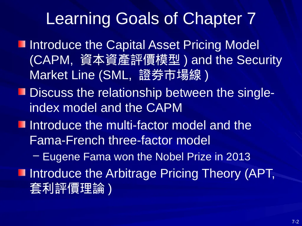
Introduce the Capital Asset Pricing Model (CAPM, 資本資產評價模型) and the Security Market Line (SML, 證券市場線)
Discuss the relationship between the single-index model and the CAPM
Introduce the multi-factor model and the Fama-French three-factor model
Eugene Fama won the Nobel Prize in 2013
Introduce the Arbitrage Pricing Theory (APT, 套利評價理論) Learning Goals of Chapter 7<br>
Discuss the relationship between the single-index model and the CAPM
Introduce the multi-factor model and the Fama-French three-factor model
Eugene Fama won the Nobel Prize in 2013
Introduce the Arbitrage Pricing Theory (APT, 套利評價理論) Learning Goals of Chapter 7<br>
03
7.1 THE CAPITAL ASSET PRICING MODEL<br>
04
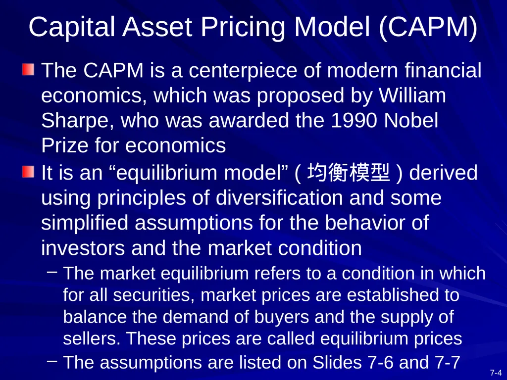
Capital Asset Pricing Model (CAPM) The CAPM is a centerpiece of modern financial economics, which was proposed by William Sharpe, who was awarded the 1990 Nobel Prize for economics
It is an “equilibrium model” (均衡模型) derived using principles of diversification and some simplified assumptions for the behavior of investors and the market condition
The market equilibrium refers to a condition in which for all securities, market prices are established to balance the demand of buyers and the supply of sellers. These prices are called equilibrium prices
The assumptions are listed on Slides 7-6 and 7-7<br>
It is an “equilibrium model” (均衡模型) derived using principles of diversification and some simplified assumptions for the behavior of investors and the market condition
The market equilibrium refers to a condition in which for all securities, market prices are established to balance the demand of buyers and the supply of sellers. These prices are called equilibrium prices
The assumptions are listed on Slides 7-6 and 7-7<br>
05
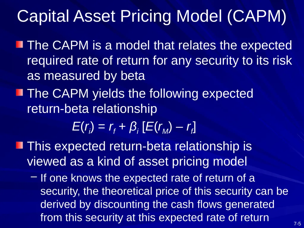
Capital Asset Pricing Model (CAPM) The CAPM is a model that relates the expected required rate of return for any security to its risk as measured by beta
The CAPM yields the following expected return-beta relationship
E(ri) = rf + βi [E(rM) – rf]
This expected return-beta relationship is viewed as a kind of asset pricing model
If one knows the expected rate of return of a security, the theoretical price of this security can be derived by discounting the cash flows generated from this security at this expected rate of return<br>
The CAPM yields the following expected return-beta relationship
E(ri) = rf + βi [E(rM) – rf]
This expected return-beta relationship is viewed as a kind of asset pricing model
If one knows the expected rate of return of a security, the theoretical price of this security can be derived by discounting the cash flows generated from this security at this expected rate of return<br>
06
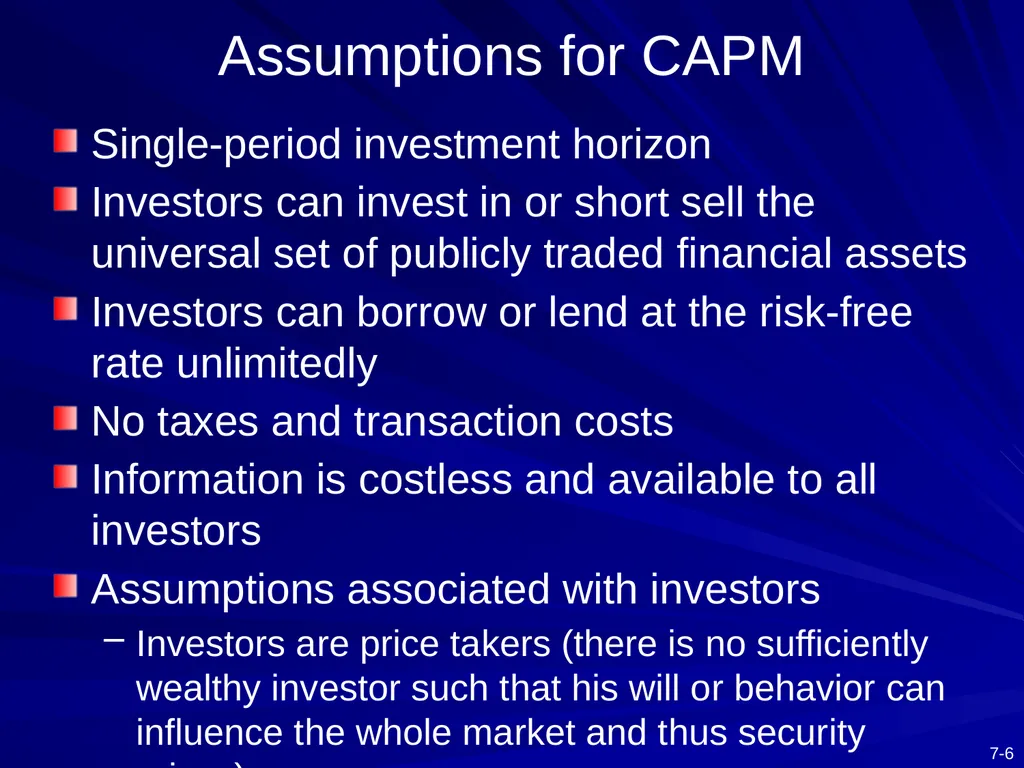
Assumptions for CAPM Single-period investment horizon
Investors can invest in or short sell the universal set of publicly traded financial assets
Investors can borrow or lend at the risk-free rate unlimitedly
No taxes and transaction costs
Information is costless and available to all investors
Assumptions associated with investors
Investors are price takers (there is no sufficiently wealthy investor such that his will or behavior can influence the whole market and thus security prices)<br>
Investors can invest in or short sell the universal set of publicly traded financial assets
Investors can borrow or lend at the risk-free rate unlimitedly
No taxes and transaction costs
Information is costless and available to all investors
Assumptions associated with investors
Investors are price takers (there is no sufficiently wealthy investor such that his will or behavior can influence the whole market and thus security prices)<br>
07
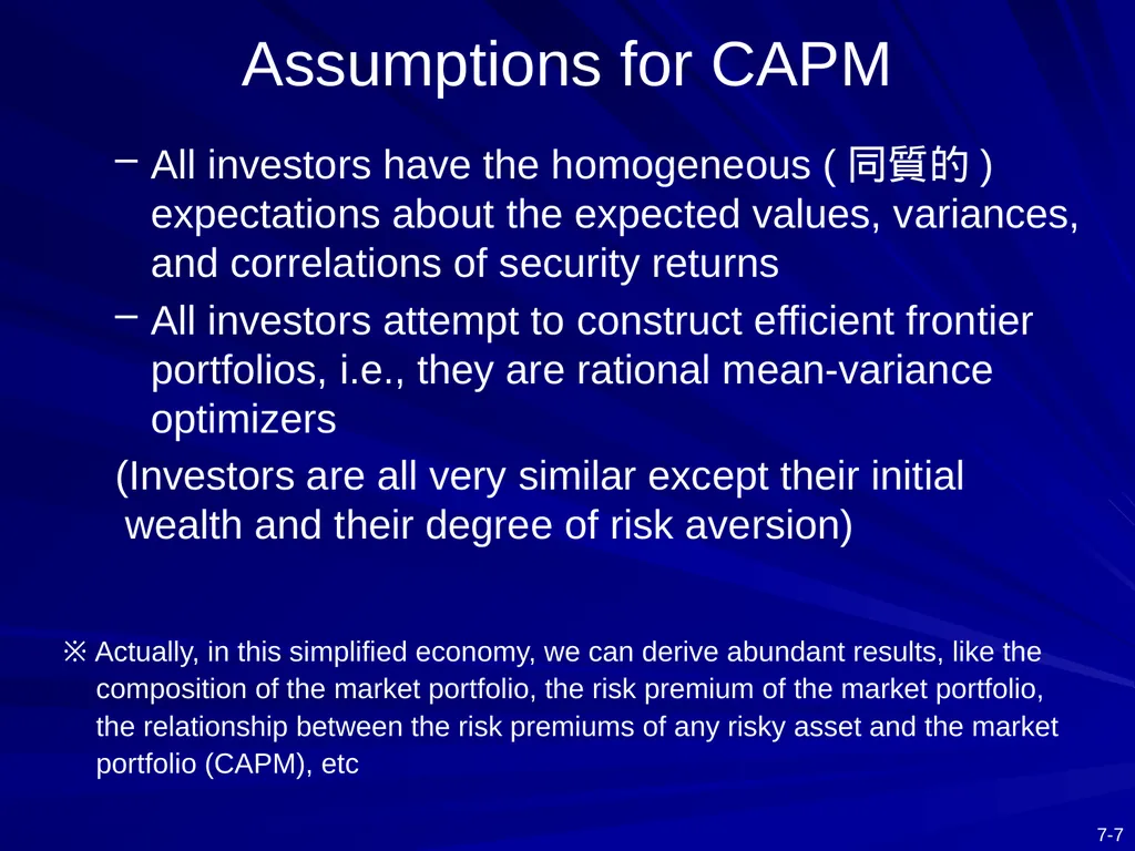
Assumptions for CAPM All investors have the homogeneous (同質的) expectations about the expected values, variances, and correlations of security returns
All investors attempt to construct efficient frontier portfolios, i.e., they are rational mean-variance optimizers
(Investors are all very similar except their initial wealth and their degree of risk aversion) ※ Actually, in this simplified economy, we can derive abundant results, like the composition of the market portfolio, the risk premium of the market portfolio, the relationship between the risk premiums of any risky asset and the market portfolio (CAPM), etc<br>
All investors attempt to construct efficient frontier portfolios, i.e., they are rational mean-variance optimizers
(Investors are all very similar except their initial wealth and their degree of risk aversion) ※ Actually, in this simplified economy, we can derive abundant results, like the composition of the market portfolio, the risk premium of the market portfolio, the relationship between the risk premiums of any risky asset and the market portfolio (CAPM), etc<br>
08
Resulting Equilibrium Conditions Identical efficient frontier
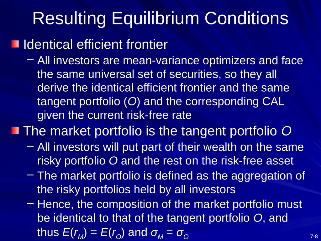
All investors are mean-variance optimizers and face the same universal set of securities, so they all derive the identical efficient frontier and the same tangent portfolio (O) and the corresponding CAL given the current risk-free rate
The market portfolio is the tangent portfolio O
All investors will put part of their wealth on the same risky portfolio O and the rest on the risk-free asset
The market portfolio is defined as the aggregation of the risky portfolios held by all investors
Hence, the composition of the market portfolio must be identical to that of the tangent portfolio O, and thus E(rM) = E(rO) and σM = σO<br>
All investors are mean-variance optimizers and face the same universal set of securities, so they all derive the identical efficient frontier and the same tangent portfolio (O) and the corresponding CAL given the current risk-free rate
The market portfolio is the tangent portfolio O
All investors will put part of their wealth on the same risky portfolio O and the rest on the risk-free asset
The market portfolio is defined as the aggregation of the risky portfolios held by all investors
Hence, the composition of the market portfolio must be identical to that of the tangent portfolio O, and thus E(rM) = E(rO) and σM = σO<br>
09
The capital market line (CML, 資本市場線)
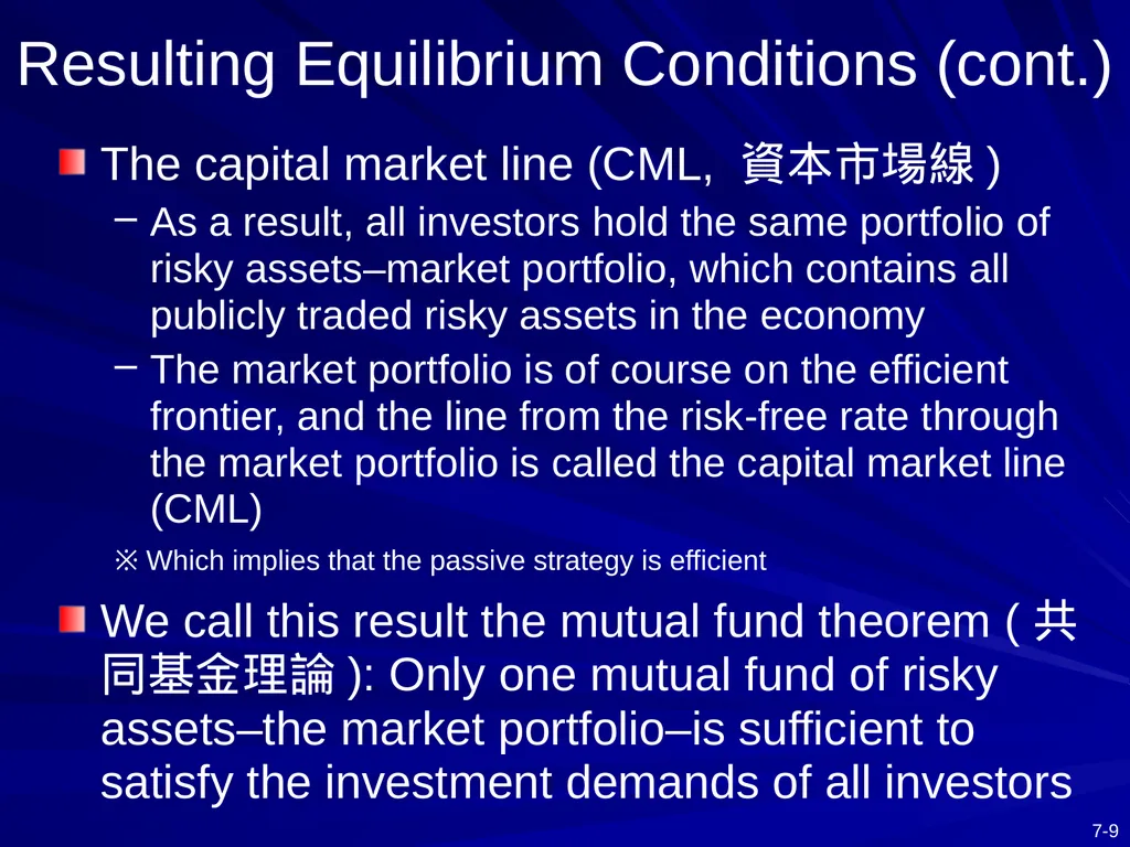
As a result, all investors hold the same portfolio of risky assets–market portfolio, which contains all publicly traded risky assets in the economy
The market portfolio is of course on the efficient frontier, and the line from the risk-free rate through the market portfolio is called the capital market line (CML)
※ Which implies that the passive strategy is efficient
We call this result the mutual fund theorem (共同基金理論): Only one mutual fund of risky assets–the market portfolio–is sufficient to satisfy the investment demands of all investors Resulting Equilibrium Conditions (cont.)<br>
As a result, all investors hold the same portfolio of risky assets–market portfolio, which contains all publicly traded risky assets in the economy
The market portfolio is of course on the efficient frontier, and the line from the risk-free rate through the market portfolio is called the capital market line (CML)
※ Which implies that the passive strategy is efficient
We call this result the mutual fund theorem (共同基金理論): Only one mutual fund of risky assets–the market portfolio–is sufficient to satisfy the investment demands of all investors Resulting Equilibrium Conditions (cont.)<br>
10
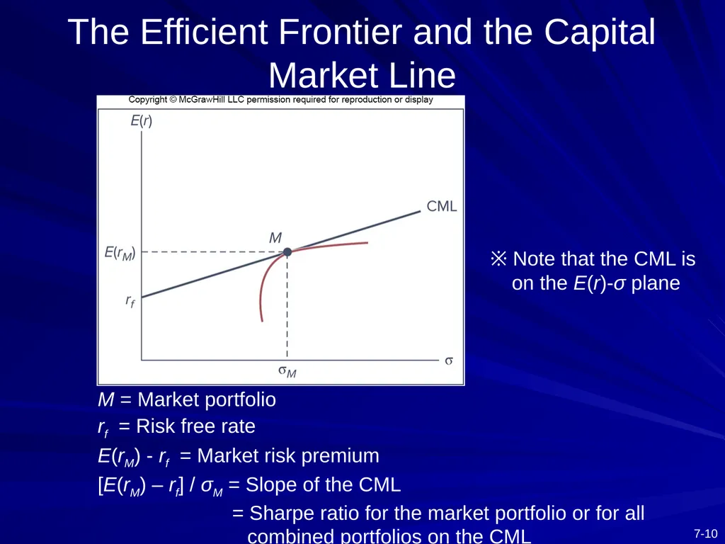
The Efficient Frontier and the Capital Market Line M = Market portfolio
rf = Risk free rate
E(rM) - rf = Market risk premium
[E(rM) – rf] / σM = Slope of the CML
= Sharpe ratio for the market portfolio or for all combined portfolios on the CML ※ Note that the CML is on the E(r)-σ plane<br>
rf = Risk free rate
E(rM) - rf = Market risk premium
[E(rM) – rf] / σM = Slope of the CML
= Sharpe ratio for the market portfolio or for all combined portfolios on the CML ※ Note that the CML is on the E(r)-σ plane<br>
11
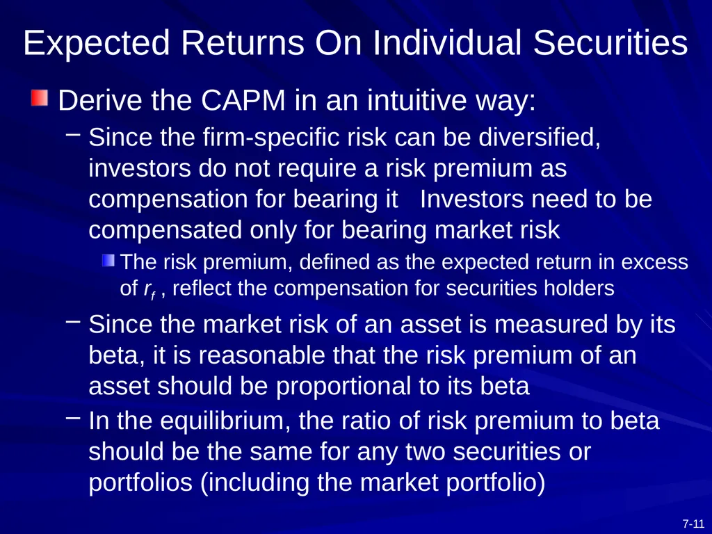
Expected Returns On Individual Securities Derive the CAPM in an intuitive way:
Since the firm-specific risk can be diversified, investors do not require a risk premium as compensation for bearing it Investors need to be compensated only for bearing market risk
The risk premium, defined as the expected return in excess of rf , reflect the compensation for securities holders
Since the market risk of an asset is measured by its beta, it is reasonable that the risk premium of an asset should be proportional to its beta
In the equilibrium, the ratio of risk premium to beta should be the same for any two securities or portfolios (including the market portfolio)<br>
Since the firm-specific risk can be diversified, investors do not require a risk premium as compensation for bearing it Investors need to be compensated only for bearing market risk
The risk premium, defined as the expected return in excess of rf , reflect the compensation for securities holders
Since the market risk of an asset is measured by its beta, it is reasonable that the risk premium of an asset should be proportional to its beta
In the equilibrium, the ratio of risk premium to beta should be the same for any two securities or portfolios (including the market portfolio)<br>
12
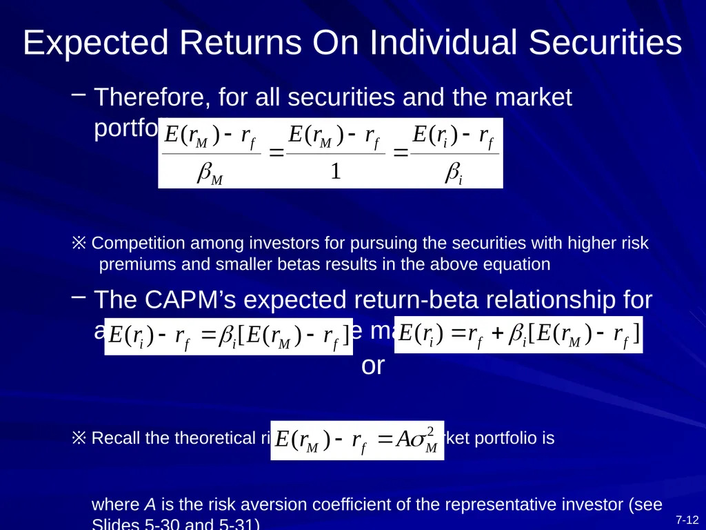
Therefore, for all securities and the market portfolio,
※ Competition among investors for pursuing the securities with higher risk premiums and smaller betas results in the above equation
The CAPM’s expected return-beta relationship for any security (except the market portfolio)
or
※ Recall the theoretical risk premium of the market portfolio is
where A is the risk aversion coefficient of the representative investor (see Slides 5-30 and 5-31) Expected Returns On Individual Securities<br>
※ Competition among investors for pursuing the securities with higher risk premiums and smaller betas results in the above equation
The CAPM’s expected return-beta relationship for any security (except the market portfolio)
or
※ Recall the theoretical risk premium of the market portfolio is
where A is the risk aversion coefficient of the representative investor (see Slides 5-30 and 5-31) Expected Returns On Individual Securities<br>
13
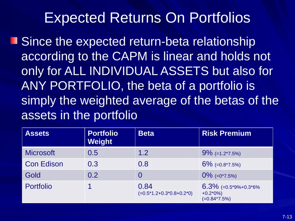
Since the expected return-beta relationship according to the CAPM is linear and holds not only for ALL INDIVIDUAL ASSETS but also for ANY PORTFOLIO, the beta of a portfolio is simply the weighted average of the betas of the assets in the portfolio Expected Returns On Portfolios<br>
14
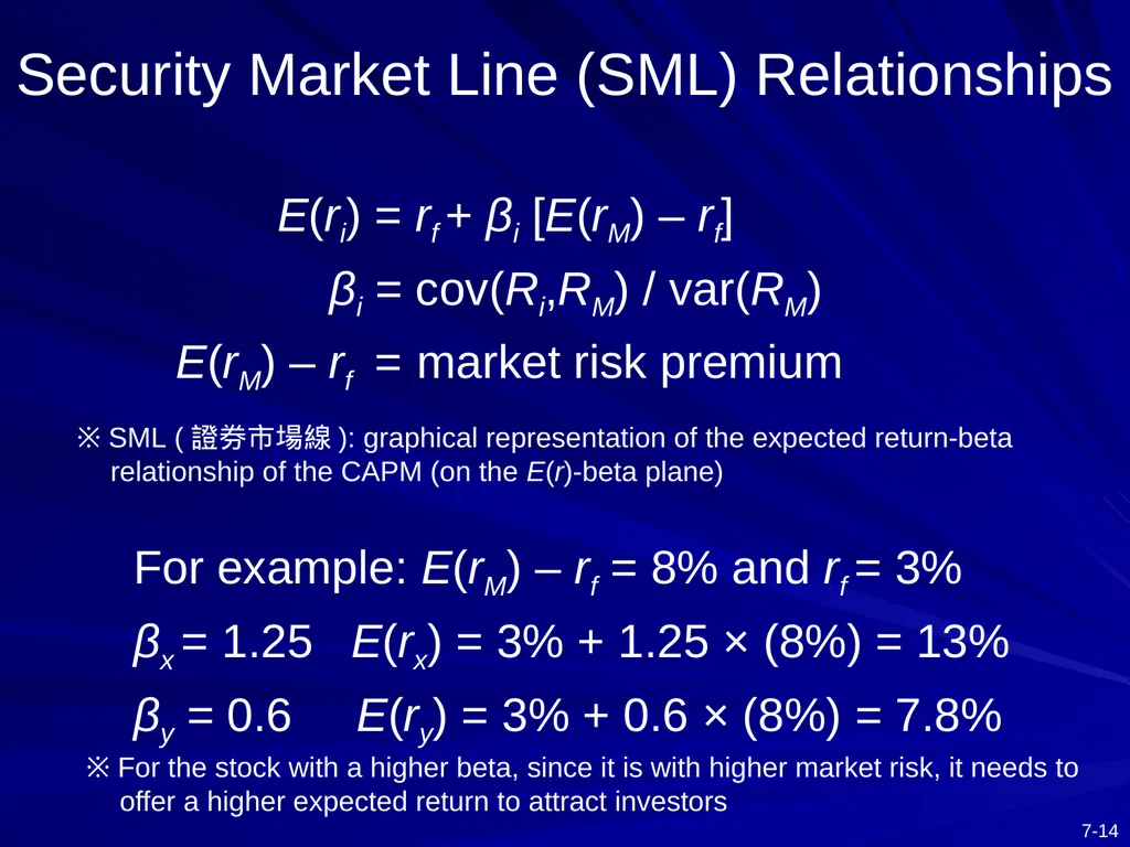
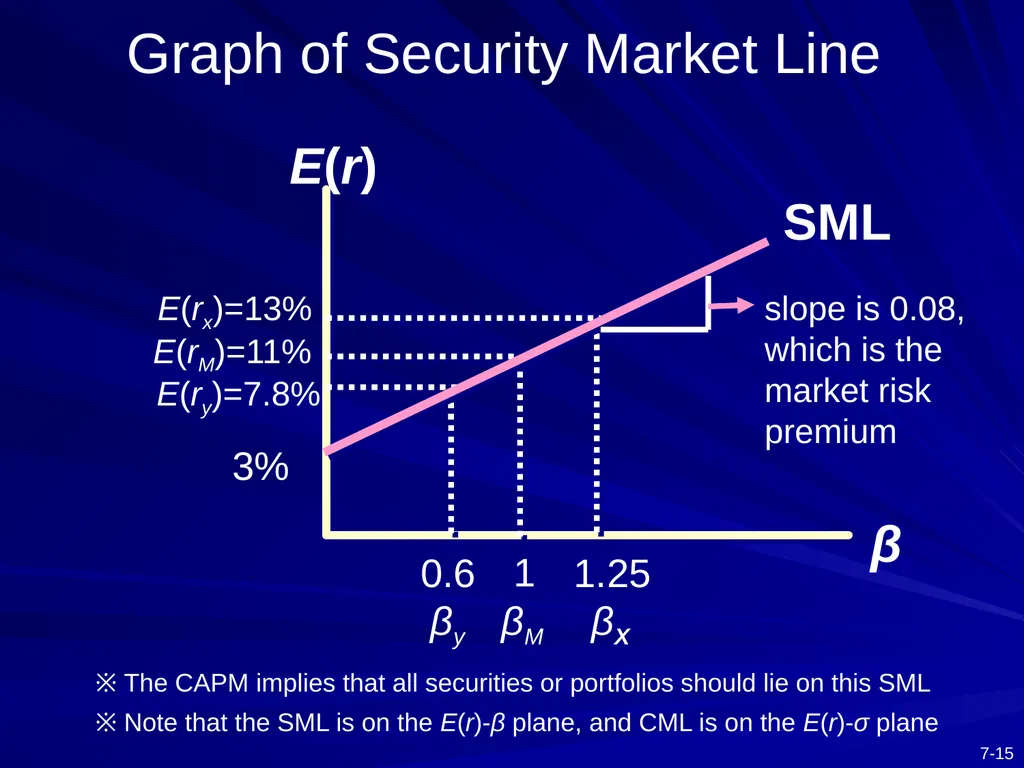
Security Market Line (SML) Relationships E(ri) = rf + βi [E(rM) – rf]
βi = cov(Ri,RM) / var(RM)
E(rM) – rf = market risk premium
For example: E(rM) – rf = 8% and rf = 3%
βx = 1.25 E(rx) = 3% + 1.25 × (8%) = 13%
βy = 0.6 E(ry) = 3% + 0.6 × (8%) = 7.8% ※ SML (證券市場線): graphical representation of the expected return-beta relationship of the CAPM (on the E(r)-beta plane) ※ For the stock with a higher beta, since it is with higher market risk, it needs to offer a higher expected return to attract investors<br>
βi = cov(Ri,RM) / var(RM)
E(rM) – rf = market risk premium
For example: E(rM) – rf = 8% and rf = 3%
βx = 1.25 E(rx) = 3% + 1.25 × (8%) = 13%
βy = 0.6 E(ry) = 3% + 0.6 × (8%) = 7.8% ※ SML (證券市場線): graphical representation of the expected return-beta relationship of the CAPM (on the E(r)-beta plane) ※ For the stock with a higher beta, since it is with higher market risk, it needs to offer a higher expected return to attract investors<br>
15
Graph of Security Market Line ※ The CAPM implies that all securities or portfolios should lie on this SML
※ Note that the SML is on the E(r)-β plane, and CML is on the E(r)-σ plane<br>
※ Note that the SML is on the E(r)-β plane, and CML is on the E(r)-σ plane<br>
16
In reality, not all securities lie on the SML
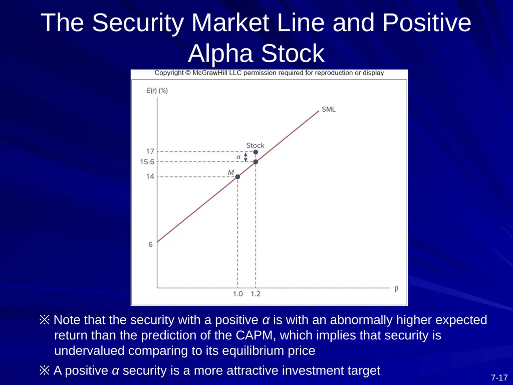
Underpriced (overpriced) stocks plot above (below) the SML: Given their betas, their expected rates of return are higher (lower) than the predication by the CAPM and thus the securities are underpriced (overpriced) (see the next slide)
The difference between the expected and actually rate of return on a security is the abnormal rate of return (異常報酬率) on this security, which is often denoted as alpha (α)
Use SML as benchmark for fair return (or hurdle rate (最低報酬率)) for risky assets or portfolios Applications of the CAPM<br>
Underpriced (overpriced) stocks plot above (below) the SML: Given their betas, their expected rates of return are higher (lower) than the predication by the CAPM and thus the securities are underpriced (overpriced) (see the next slide)
The difference between the expected and actually rate of return on a security is the abnormal rate of return (異常報酬率) on this security, which is often denoted as alpha (α)
Use SML as benchmark for fair return (or hurdle rate (最低報酬率)) for risky assets or portfolios Applications of the CAPM<br>
17
The Security Market Line and Positive Alpha Stock ※ Note that the security with a positive α is with an abnormally higher expected return than the prediction of the CAPM, which implies that security is undervalued comparing to its equilibrium price
※ A positive α security is a more attractive investment target<br>
※ A positive α security is a more attractive investment target<br>
18
The most important goal for investment is to smooth the individual’s consumption
Suppose RM can reflect the business cycle, i.e., RM ↑, then individual’s consumption ↑ due to the booming economy
βA > 0 cov(RA,RM) > 0 RM ↑, RA ↑ and thus bring more consumption, and RM ↓, RA ↓ and thus reduce consumption
βB < 0 cov(RB,RM) < 0 RM ↑, RB ↓ and thus reduce consumption, and RM ↓, RB ↑ and thus bring more consumption
From the viewpoint of smoothing consumption, individuals prefer B and thus bid up the price of B, which implies a lower expected return of B in the equilibrium
On the contrary, individuals do not like A, so the price of A decreases, which implies a higher expected return of A
Preference for smoothing consumption is consistent with the CAPM CAPM vs. Smoothing Consumption<br>
Suppose RM can reflect the business cycle, i.e., RM ↑, then individual’s consumption ↑ due to the booming economy
βA > 0 cov(RA,RM) > 0 RM ↑, RA ↑ and thus bring more consumption, and RM ↓, RA ↓ and thus reduce consumption
βB < 0 cov(RB,RM) < 0 RM ↑, RB ↓ and thus reduce consumption, and RM ↓, RB ↑ and thus bring more consumption
From the viewpoint of smoothing consumption, individuals prefer B and thus bid up the price of B, which implies a lower expected return of B in the equilibrium
On the contrary, individuals do not like A, so the price of A decreases, which implies a higher expected return of A
Preference for smoothing consumption is consistent with the CAPM CAPM vs. Smoothing Consumption<br>
19
CAPM implies that the passive strategy
Everyone invests in the combination of the market portfolio and the risk-free asset All investors adopt the passive strategy
Several flaws of CAPM
Unreal assumptions, e.g., homogeneous expectations of security returns and variances, borrowing funds at the risk-free interest rate
Logical inconsistency:
If a passive strategy is costless and efficient, why would anyone follow an active strategy?
If no one does any security analysis, what brings about the efficiency of the market portfolio? Complementary Issues Associated CAPM<br>
Everyone invests in the combination of the market portfolio and the risk-free asset All investors adopt the passive strategy
Several flaws of CAPM
Unreal assumptions, e.g., homogeneous expectations of security returns and variances, borrowing funds at the risk-free interest rate
Logical inconsistency:
If a passive strategy is costless and efficient, why would anyone follow an active strategy?
If no one does any security analysis, what brings about the efficiency of the market portfolio? Complementary Issues Associated CAPM<br>
20
7.2 THE CAPM AND INDEX MODELS<br>
21
Estimating the Index Model The CAPM has two limitations:
It relies on the theoretical market portfolio, which includes all assets (not only domestic stocks but also bonds, foreign stocks and bonds, real estates, etc.)
It deals with expected returns, which cannot be observed in advance in the market
For the single index model (單一指數模型)
The stock index return, rather than the performance of the theoretical market portfolio, is employed to approximate the market factor of the economy
In addition, the index model is based on actually realized returns<br>
It relies on the theoretical market portfolio, which includes all assets (not only domestic stocks but also bonds, foreign stocks and bonds, real estates, etc.)
It deals with expected returns, which cannot be observed in advance in the market
For the single index model (單一指數模型)
The stock index return, rather than the performance of the theoretical market portfolio, is employed to approximate the market factor of the economy
In addition, the index model is based on actually realized returns<br>
22
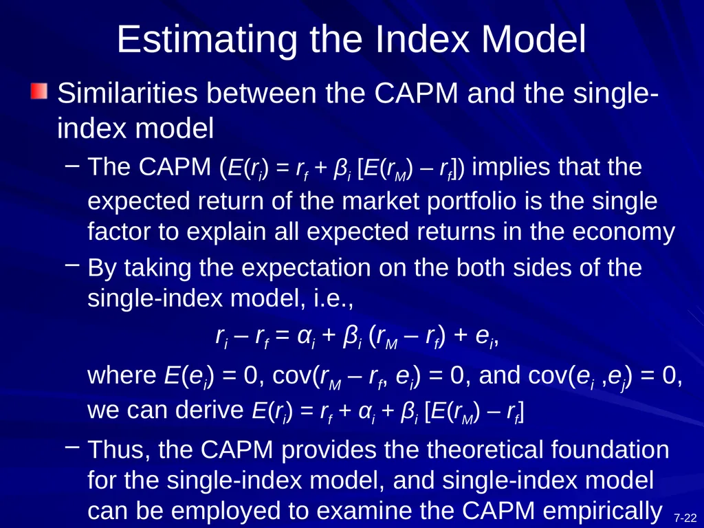
Similarities between the CAPM and the single-index model
The CAPM (E(ri) = rf + βi [E(rM) – rf]) implies that the expected return of the market portfolio is the single factor to explain all expected returns in the economy
By taking the expectation on the both sides of the single-index model, i.e.,
ri – rf = αi + βi (rM – rf) + ei,
where E(ei) = 0, cov(rM – rf, ei) = 0, and cov(ei ,ej) = 0, we can derive E(ri) = rf + αi + βi [E(rM) – rf]
Thus, the CAPM provides the theoretical foundation for the single-index model, and single-index model can be employed to examine the CAPM empirically Estimating the Index Model<br>
The CAPM (E(ri) = rf + βi [E(rM) – rf]) implies that the expected return of the market portfolio is the single factor to explain all expected returns in the economy
By taking the expectation on the both sides of the single-index model, i.e.,
ri – rf = αi + βi (rM – rf) + ei,
where E(ei) = 0, cov(rM – rf, ei) = 0, and cov(ei ,ej) = 0, we can derive E(ri) = rf + αi + βi [E(rM) – rf]
Thus, the CAPM provides the theoretical foundation for the single-index model, and single-index model can be employed to examine the CAPM empirically Estimating the Index Model<br>
23
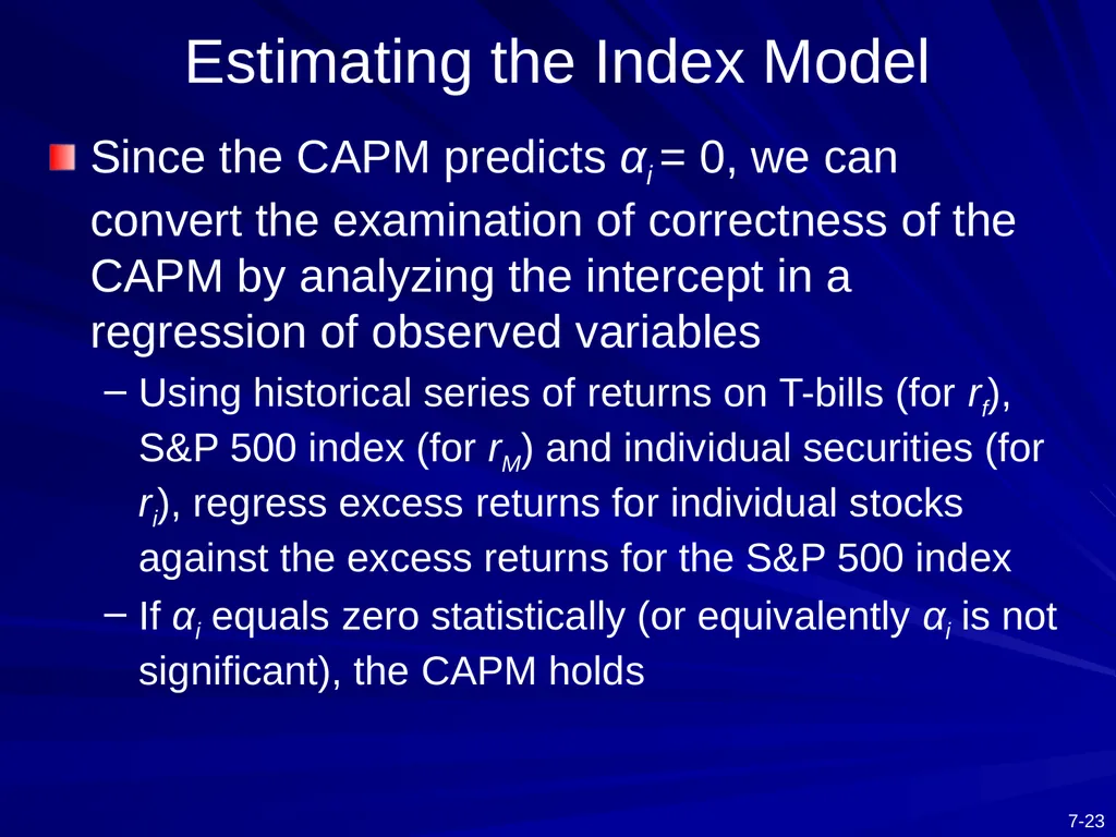
Estimating the Index Model Since the CAPM predicts αi = 0, we can convert the examination of correctness of the CAPM by analyzing the intercept in a regression of observed variables
Using historical series of returns on T-bills (for rf), S&P 500 index (for rM) and individual securities (for ri), regress excess returns for individual stocks against the excess returns for the S&P 500 index
If αi equals zero statistically (or equivalently αi is not significant), the CAPM holds<br>
Using historical series of returns on T-bills (for rf), S&P 500 index (for rM) and individual securities (for ri), regress excess returns for individual stocks against the excess returns for the S&P 500 index
If αi equals zero statistically (or equivalently αi is not significant), the CAPM holds<br>
24
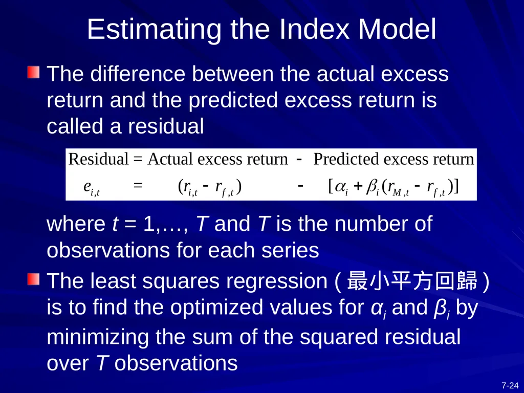
Estimating the Index Model The difference between the actual excess return and the predicted excess return is called a residual
where t = 1,…, T and T is the number of observations for each series
The least squares regression (最小平方回歸) is to find the optimized values for αi and βi by minimizing the sum of the squared residual over T observations<br>
where t = 1,…, T and T is the number of observations for each series
The least squares regression (最小平方回歸) is to find the optimized values for αi and βi by minimizing the sum of the squared residual over T observations<br>
25
We use the monthly series over Jan/2006 -Dec/2010 for the T-bills rate, the Google stock price, and the S&P 500 index for regression (For Google and S&P 500, their rates of return must be adjusted for stock splits, stock dividends, and cash dividends)
The unadjusted price series counts only capital gains, but here we need total returns
We can calculate the excess returns of the Google stock and the S&P 500 index for each month, and plots each pair of these excess returns on the xy-plane (see the scatter diagram on the next slide) Estimating the Index Model<br>
The unadjusted price series counts only capital gains, but here we need total returns
We can calculate the excess returns of the Google stock and the S&P 500 index for each month, and plots each pair of these excess returns on the xy-plane (see the scatter diagram on the next slide) Estimating the Index Model<br>
26
Scatter Diagram (點散圖) and the Security Characteristic Line (證券特徵線) for Google ※ The security characteristic line (SCL) describes the linear function of security’s expected excess return with respect to the excess return on the market index
※ The level of dispersion of the points around the SCL measures firm-specific risk. The corresponding statistic is sd(ei) = σe<br>
※ The level of dispersion of the points around the SCL measures firm-specific risk. The corresponding statistic is sd(ei) = σe<br>
27
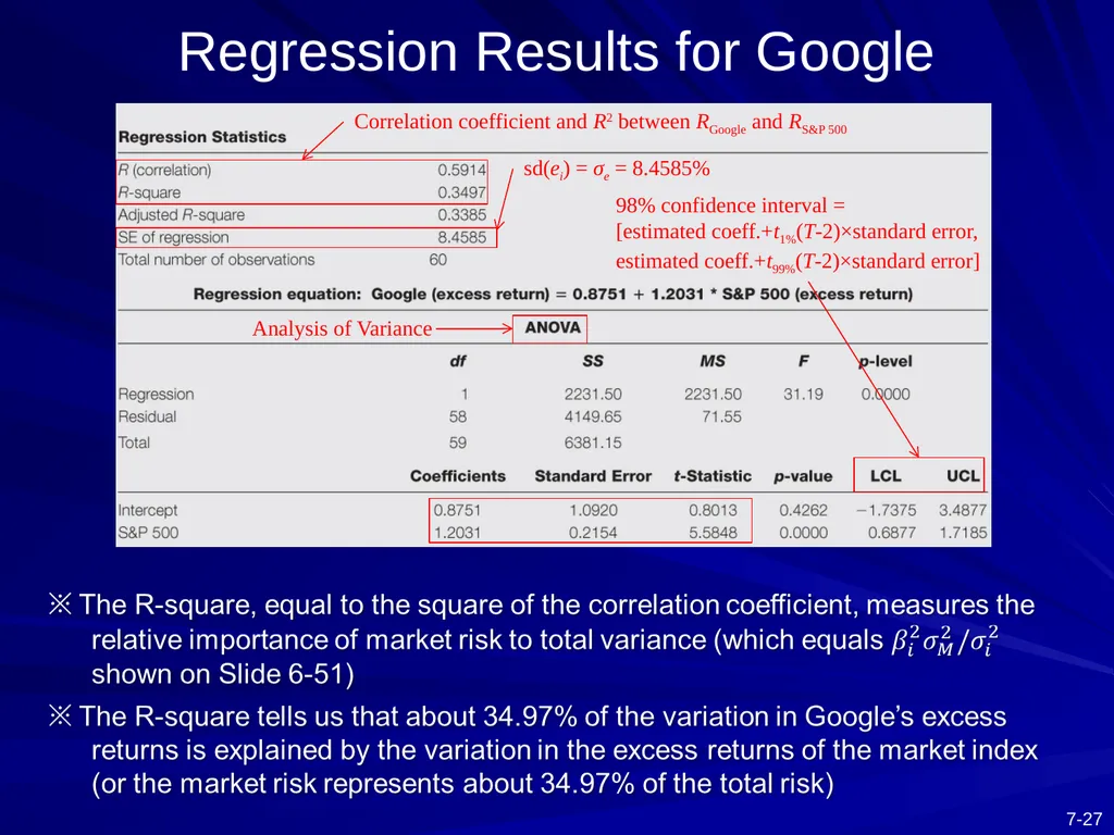
Regression Results for Google<br>
28
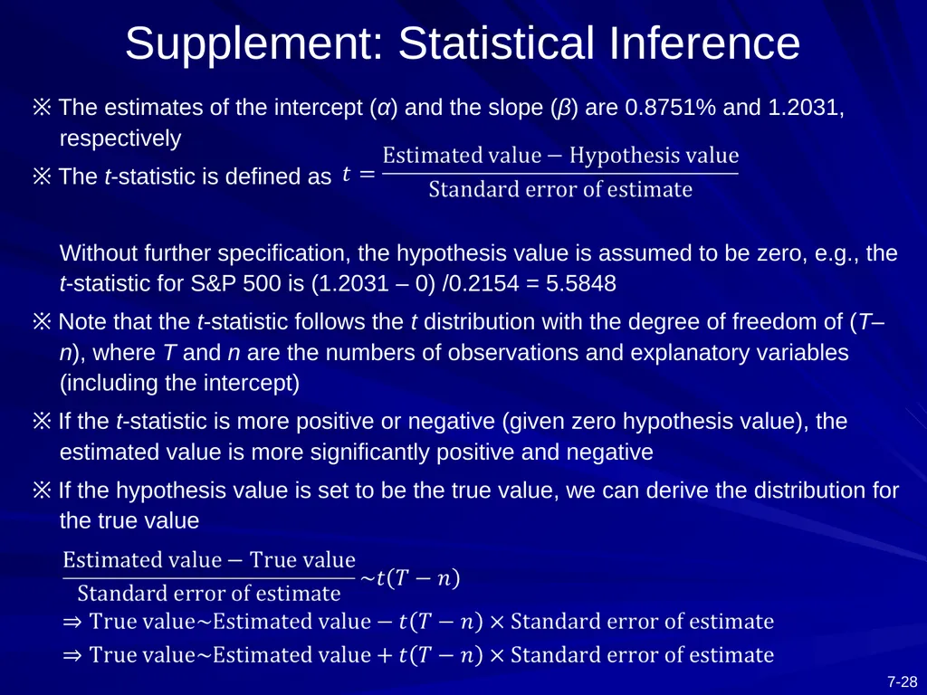
※ The estimates of the intercept (α) and the slope (β) are 0.8751% and 1.2031, respectively
※ The t-statistic is defined as
Without further specification, the hypothesis value is assumed to be zero, e.g., the t-statistic for S&P 500 is (1.2031 – 0) /0.2154 = 5.5848
※ Note that the t-statistic follows the t distribution with the degree of freedom of (T–n), where T and n are the numbers of observations and explanatory variables (including the intercept)
※ If the t-statistic is more positive or negative (given zero hypothesis value), the estimated value is more significantly positive and negative
※ If the hypothesis value is set to be the true value, we can derive the distribution for the true value Supplement: Statistical Inference<br>
※ The t-statistic is defined as
Without further specification, the hypothesis value is assumed to be zero, e.g., the t-statistic for S&P 500 is (1.2031 – 0) /0.2154 = 5.5848
※ Note that the t-statistic follows the t distribution with the degree of freedom of (T–n), where T and n are the numbers of observations and explanatory variables (including the intercept)
※ If the t-statistic is more positive or negative (given zero hypothesis value), the estimated value is more significantly positive and negative
※ If the hypothesis value is set to be the true value, we can derive the distribution for the true value Supplement: Statistical Inference<br>
29
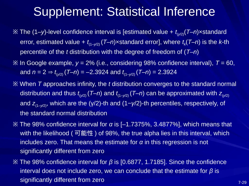
※ The (1–y)-level confidence interval is [estimated value + t(y/2)(T–n)×standard error, estimated value + t(1–y/2) (T–n)×standard error], where tk(T–n) is the k-th percentile of the t distribution with the degree of freedom of (T–n)
※ In Google example, y = 2% (i.e., considering 98% confidence interval), T = 60, and n = 2 t(y/2) (T–n) = –2.3924 and t(1–y/2) (T–n) = 2.3924
※ When T approaches infinity, the t distribution converges to the standard normal distribution and thus t(y/2) (T–n) and t(1–y/2) (T–n) can be approximated with z(y/2) and z(1–y/2), which are the (γ/2)-th and (1−γ/2)-th percentiles, respectively, of the standard normal distribution
※ The 98% confidence interval for α is [–1.7375%, 3.4877%], which means that with the likelihood (可能性) of 98%, the true alpha lies in this interval, which includes zero. That means the estimate for α in this regression is not significantly different from zero
※ The 98% confidence interval for β is [0.6877, 1.7185]. Since the confidence interval does not include zero, we can conclude that the estimate for β is significantly different from zero Supplement: Statistical Inference<br>
※ In Google example, y = 2% (i.e., considering 98% confidence interval), T = 60, and n = 2 t(y/2) (T–n) = –2.3924 and t(1–y/2) (T–n) = 2.3924
※ When T approaches infinity, the t distribution converges to the standard normal distribution and thus t(y/2) (T–n) and t(1–y/2) (T–n) can be approximated with z(y/2) and z(1–y/2), which are the (γ/2)-th and (1−γ/2)-th percentiles, respectively, of the standard normal distribution
※ The 98% confidence interval for α is [–1.7375%, 3.4877%], which means that with the likelihood (可能性) of 98%, the true alpha lies in this interval, which includes zero. That means the estimate for α in this regression is not significantly different from zero
※ The 98% confidence interval for β is [0.6877, 1.7185]. Since the confidence interval does not include zero, we can conclude that the estimate for β is significantly different from zero Supplement: Statistical Inference<br>
30
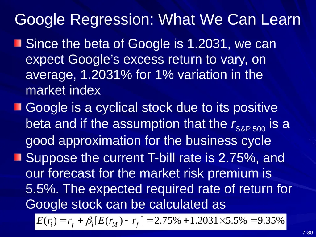
Google Regression: What We Can Learn Since the beta of Google is 1.2031, we can expect Google’s excess return to vary, on average, 1.2031% for 1% variation in the market index
Google is a cyclical stock due to its positive beta and if the assumption that the rS&P 500 is a good approximation for the business cycle
Suppose the current T-bill rate is 2.75%, and our forecast for the market risk premium is 5.5%. The expected required rate of return for Google stock can be calculated as<br>
Google is a cyclical stock due to its positive beta and if the assumption that the rS&P 500 is a good approximation for the business cycle
Suppose the current T-bill rate is 2.75%, and our forecast for the market risk premium is 5.5%. The expected required rate of return for Google stock can be calculated as<br>
31
7.3 THE CAPM AND THE REAL WORLD<br>
32
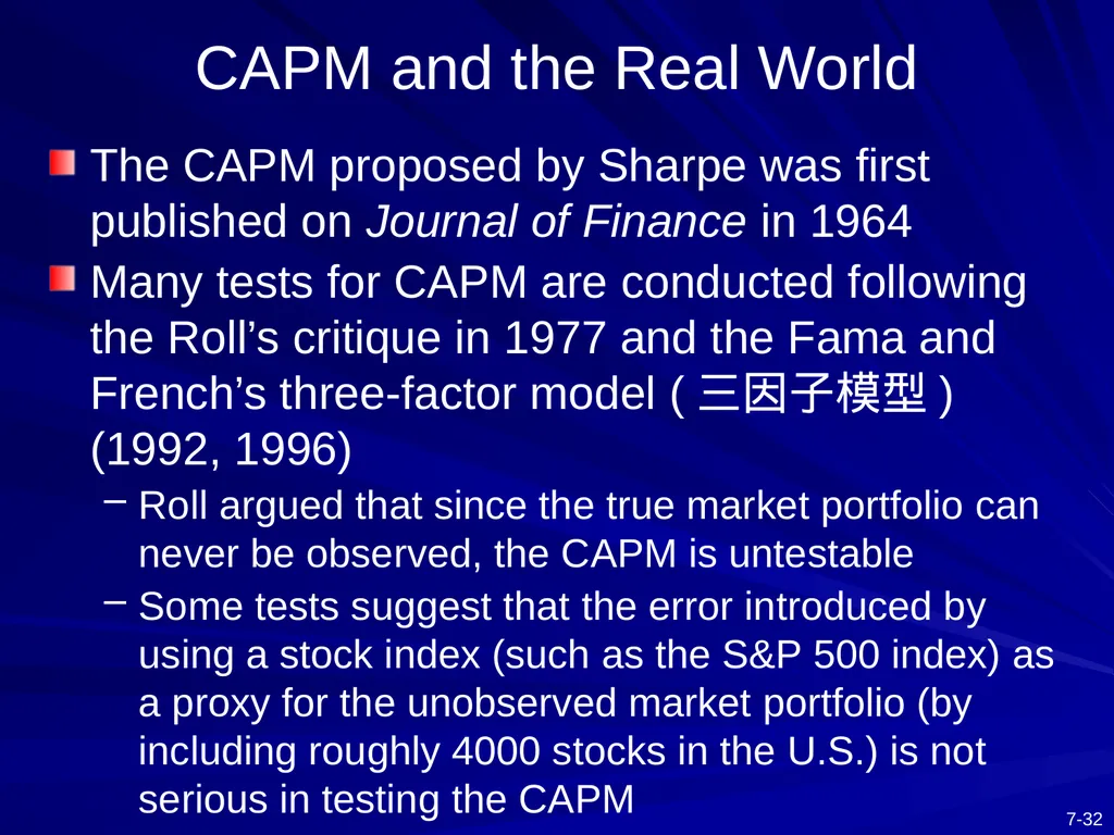
CAPM and the Real World The CAPM proposed by Sharpe was first published on Journal of Finance in 1964
Many tests for CAPM are conducted following the Roll’s critique in 1977 and the Fama and French’s three-factor model (三因子模型) (1992, 1996)
Roll argued that since the true market portfolio can never be observed, the CAPM is untestable
Some tests suggest that the error introduced by using a stock index (such as the S&P 500 index) as a proxy for the unobserved market portfolio (by including roughly 4000 stocks in the U.S.) is not serious in testing the CAPM<br>
Many tests for CAPM are conducted following the Roll’s critique in 1977 and the Fama and French’s three-factor model (三因子模型) (1992, 1996)
Roll argued that since the true market portfolio can never be observed, the CAPM is untestable
Some tests suggest that the error introduced by using a stock index (such as the S&P 500 index) as a proxy for the unobserved market portfolio (by including roughly 4000 stocks in the U.S.) is not serious in testing the CAPM<br>
33
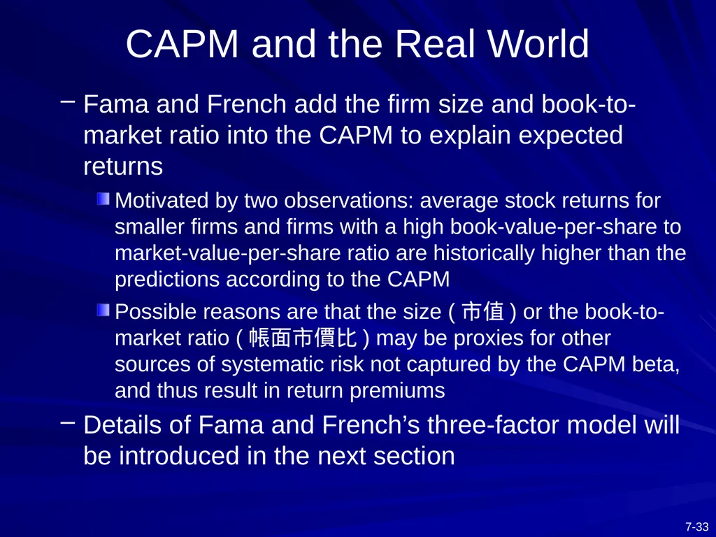
CAPM and the Real World Fama and French add the firm size and book-to-market ratio into the CAPM to explain expected returns
Motivated by two observations: average stock returns for smaller firms and firms with a high book-value-per-share to market-value-per-share ratio are historically higher than the predictions according to the CAPM
Possible reasons are that the size (市值) or the book-to-market ratio (帳面市價比) may be proxies for other sources of systematic risk not captured by the CAPM beta, and thus result in return premiums
Details of Fama and French’s three-factor model will be introduced in the next section<br>
Motivated by two observations: average stock returns for smaller firms and firms with a high book-value-per-share to market-value-per-share ratio are historically higher than the predictions according to the CAPM
Possible reasons are that the size (市值) or the book-to-market ratio (帳面市價比) may be proxies for other sources of systematic risk not captured by the CAPM beta, and thus result in return premiums
Details of Fama and French’s three-factor model will be introduced in the next section<br>
34
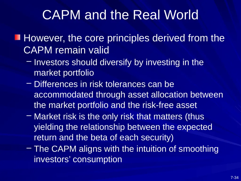
CAPM and the Real World However, the core principles derived from the CAPM remain valid
Investors should diversify by investing in the market portfolio
Differences in risk tolerances can be accommodated through asset allocation between the market portfolio and the risk-free asset
Market risk is the only risk that matters (thus yielding the relationship between the expected return and the beta of each security)
The CAPM aligns with the intuition of smoothing investors’ consumption<br>
Investors should diversify by investing in the market portfolio
Differences in risk tolerances can be accommodated through asset allocation between the market portfolio and the risk-free asset
Market risk is the only risk that matters (thus yielding the relationship between the expected return and the beta of each security)
The CAPM aligns with the intuition of smoothing investors’ consumption<br>
35
7.4 MULTIFACTOR MODELS AND THE CAPM<br>
36
Multifactor Models The systematic risk may be not from one source in reality
It is obvious that developing models that allow for several systematic risks can provide better descriptions of security returns
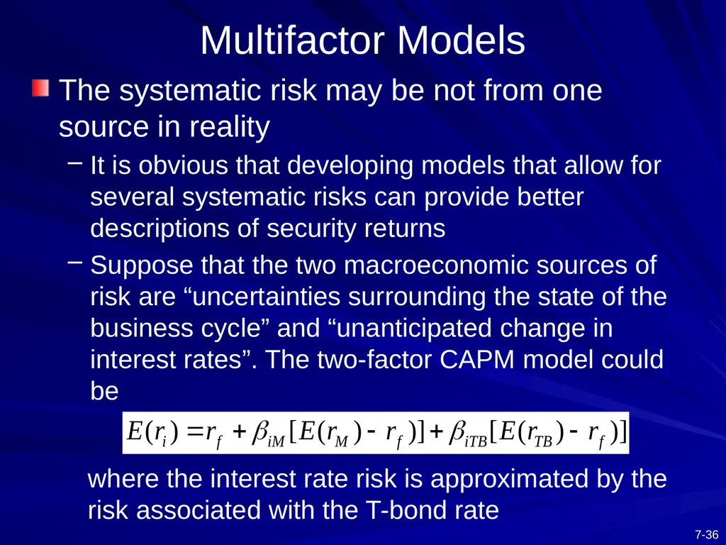
Suppose that the two macroeconomic sources of risk are “uncertainties surrounding the state of the business cycle” and “unanticipated change in interest rates”. The two-factor CAPM model could be
where the interest rate risk is approximated by the risk associated with the T-bond rate<br>
It is obvious that developing models that allow for several systematic risks can provide better descriptions of security returns
Suppose that the two macroeconomic sources of risk are “uncertainties surrounding the state of the business cycle” and “unanticipated change in interest rates”. The two-factor CAPM model could be
where the interest rate risk is approximated by the risk associated with the T-bond rate<br>
37
Multifactor Models An example for the above two-factor CAPM
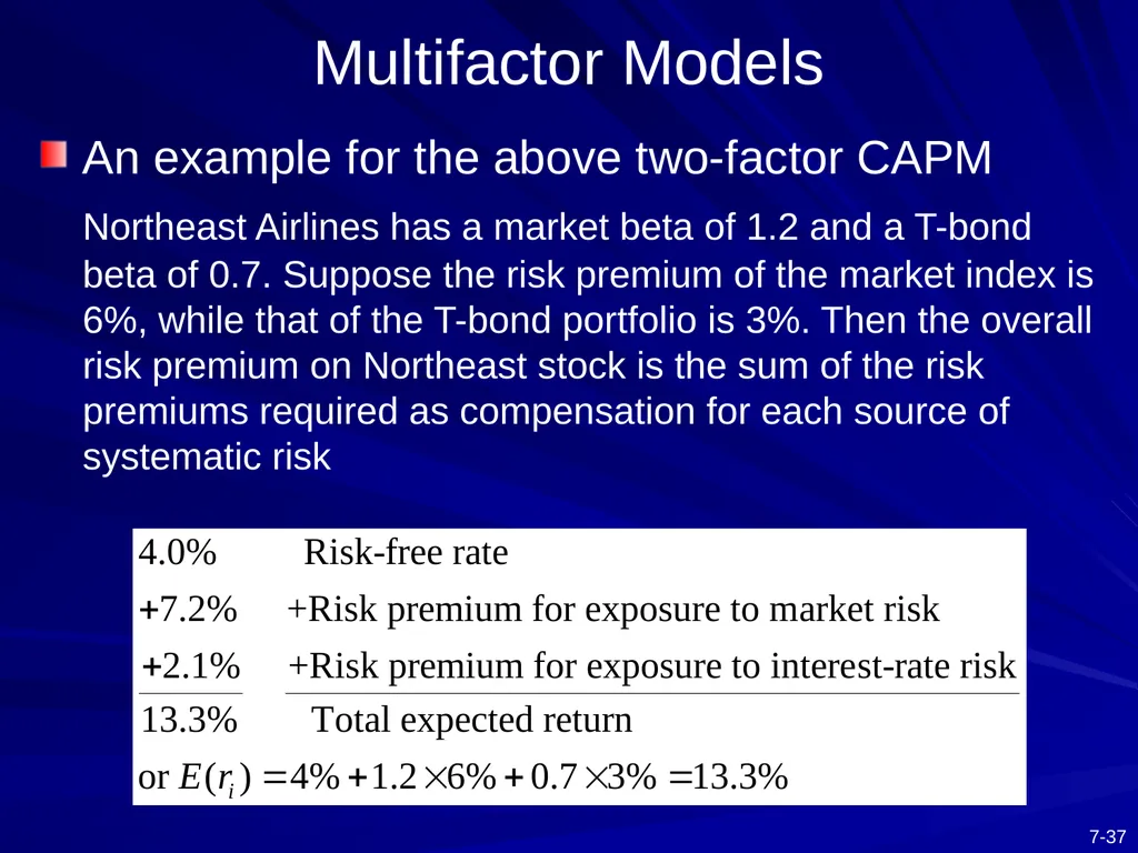
Northeast Airlines has a market beta of 1.2 and a T-bond beta of 0.7. Suppose the risk premium of the market index is 6%, while that of the T-bond portfolio is 3%. Then the overall risk premium on Northeast stock is the sum of the risk premiums required as compensation for each source of systematic risk<br>
Northeast Airlines has a market beta of 1.2 and a T-bond beta of 0.7. Suppose the risk premium of the market index is 6%, while that of the T-bond portfolio is 3%. Then the overall risk premium on Northeast stock is the sum of the risk premiums required as compensation for each source of systematic risk<br>
38
Fama-French Three-Factor Model How to identify meaningful factors to increase the explanatory or predictive power of the CAPM is still an unsolved problem
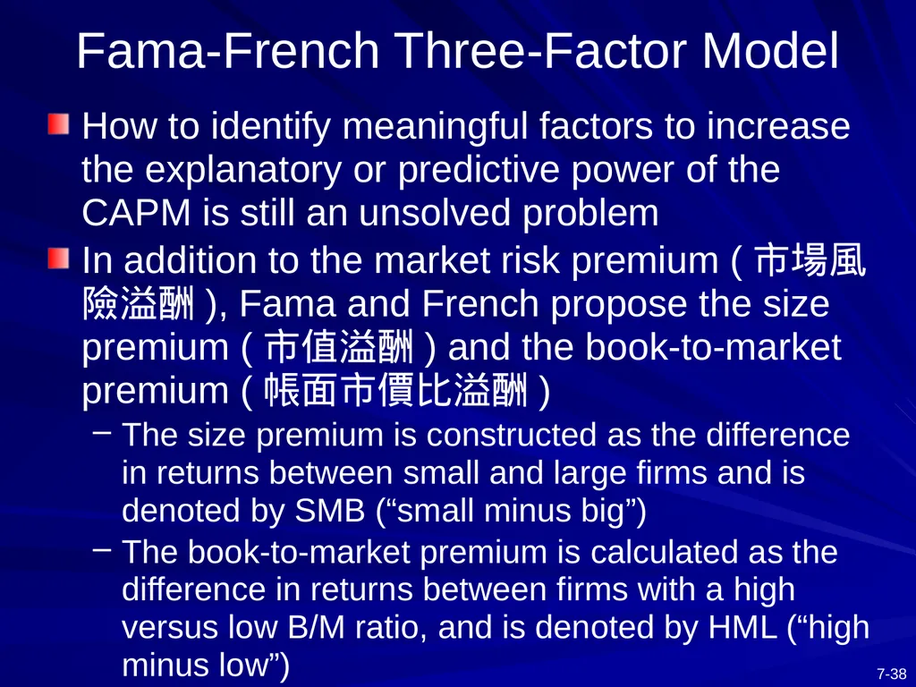
In addition to the market risk premium (市場風險溢酬), Fama and French propose the size premium (市值溢酬) and the book-to-market premium (帳面市價比溢酬)
The size premium is constructed as the difference in returns between small and large firms and is denoted by SMB (“small minus big”)
The book-to-market premium is calculated as the difference in returns between firms with a high versus low B/M ratio, and is denoted by HML (“high minus low”)<br>
In addition to the market risk premium (市場風險溢酬), Fama and French propose the size premium (市值溢酬) and the book-to-market premium (帳面市價比溢酬)
The size premium is constructed as the difference in returns between small and large firms and is denoted by SMB (“small minus big”)
The book-to-market premium is calculated as the difference in returns between firms with a high versus low B/M ratio, and is denoted by HML (“high minus low”)<br>
39
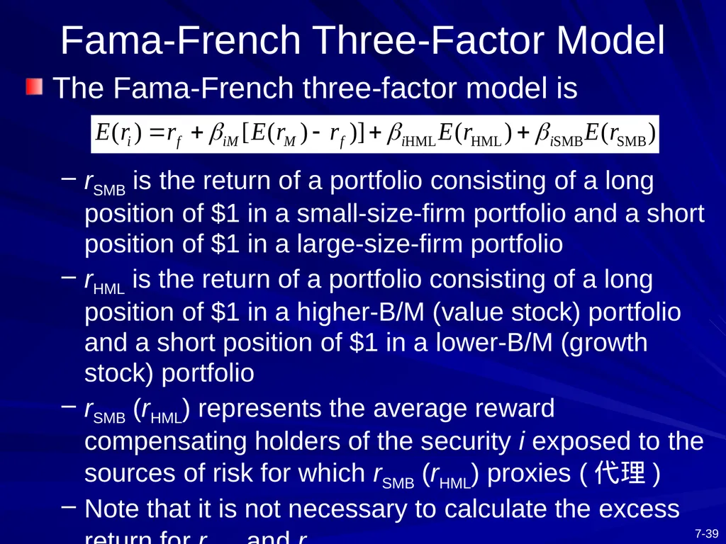
Fama-French Three-Factor Model The Fama-French three-factor model is
rSMB is the return of a portfolio consisting of a long position of $1 in a small-size-firm portfolio and a short position of $1 in a large-size-firm portfolio
rHML is the return of a portfolio consisting of a long position of $1 in a higher-B/M (value stock) portfolio and a short position of $1 in a lower-B/M (growth stock) portfolio
rSMB (rHML) represents the average reward compensating holders of the security i exposed to the sources of risk for which rSMB (rHML) proxies (代理)
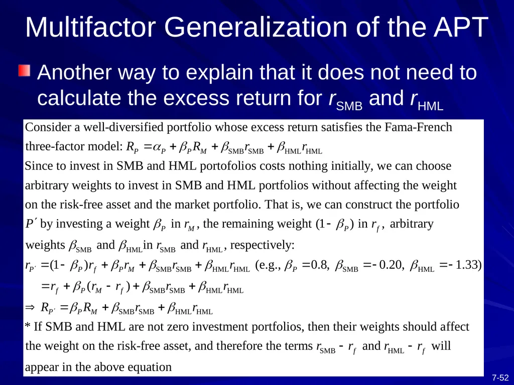
Note that it is not necessary to calculate the excess return for rSMB and rHML<br>
rSMB is the return of a portfolio consisting of a long position of $1 in a small-size-firm portfolio and a short position of $1 in a large-size-firm portfolio
rHML is the return of a portfolio consisting of a long position of $1 in a higher-B/M (value stock) portfolio and a short position of $1 in a lower-B/M (growth stock) portfolio
rSMB (rHML) represents the average reward compensating holders of the security i exposed to the sources of risk for which rSMB (rHML) proxies (代理)
Note that it is not necessary to calculate the excess return for rSMB and rHML<br>
40
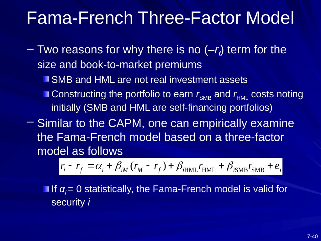
Fama-French Three-Factor Model Two reasons for why there is no (–rf) term for the size and book-to-market premiums
SMB and HML are not real investment assets
Constructing the portfolio to earn rSMB and rHML costs noting initially (SMB and HML are self-financing portfolios)
Similar to the CAPM, one can empirically examine the Fama-French model based on a three-factor model as follows
If αi = 0 statistically, the Fama-French model is valid for security i<br>
SMB and HML are not real investment assets
Constructing the portfolio to earn rSMB and rHML costs noting initially (SMB and HML are self-financing portfolios)
Similar to the CAPM, one can empirically examine the Fama-French model based on a three-factor model as follows
If αi = 0 statistically, the Fama-French model is valid for security i<br>
41
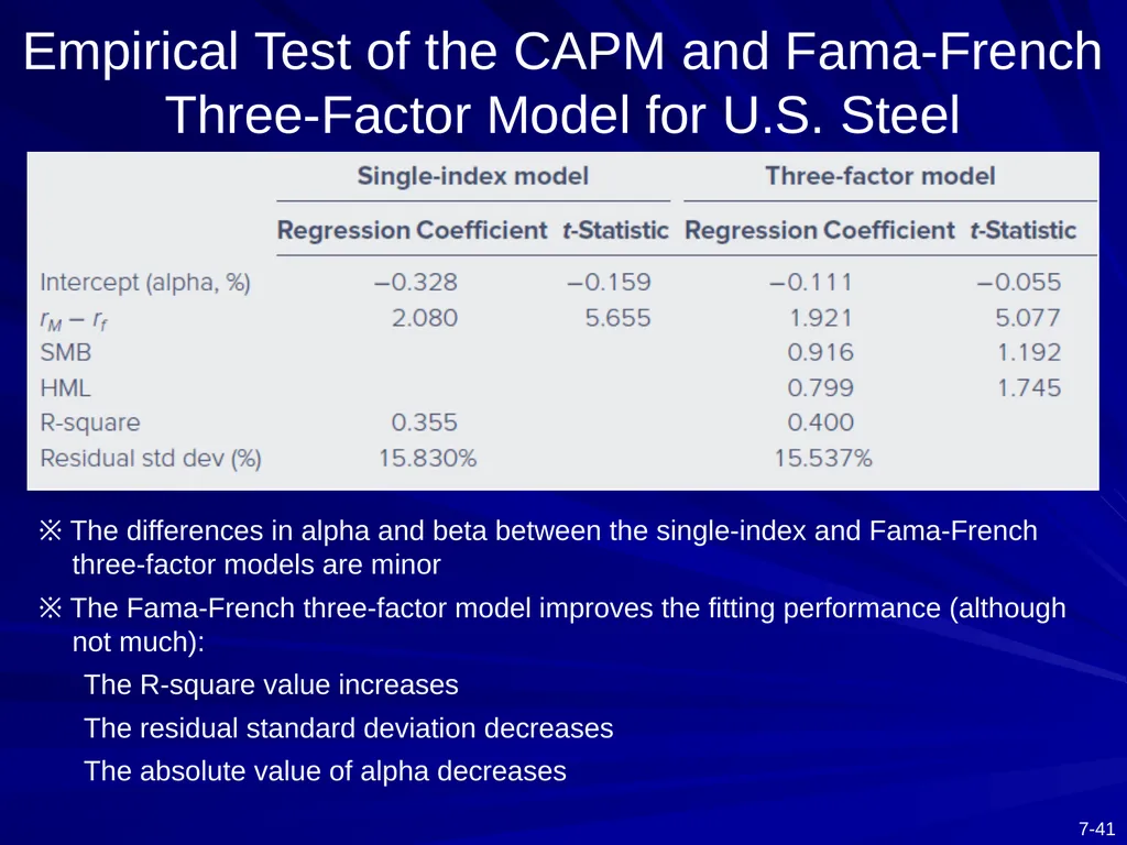
Empirical Test of the CAPM and Fama-French Three-Factor Model for U.S. Steel ※ The differences in alpha and beta between the single-index and Fama-French three-factor models are minor
※ The Fama-French three-factor model improves the fitting performance (although not much):
The R-square value increases
The residual standard deviation decreases
The absolute value of alpha decreases<br>
※ The Fama-French three-factor model improves the fitting performance (although not much):
The R-square value increases
The residual standard deviation decreases
The absolute value of alpha decreases<br>
42
Interpretation of Fama-French Three-factor Model for U.S. Steel<br>
43
7.5 ARBITRAGE PRICING THEORY<br>
44
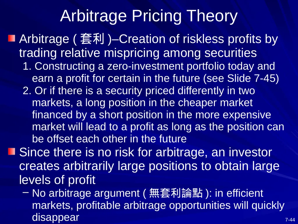
Arbitrage Pricing Theory Arbitrage (套利)–Creation of riskless profits by trading relative mispricing among securities
1. Constructing a zero-investment portfolio today and earn a profit for certain in the future (see Slide 7-45)
2. Or if there is a security priced differently in two markets, a long position in the cheaper market financed by a short position in the more expensive market will lead to a profit as long as the position can be offset each other in the future
Since there is no risk for arbitrage, an investor creates arbitrarily large positions to obtain large levels of profit
No arbitrage argument (無套利論點): in efficient markets, profitable arbitrage opportunities will quickly disappear<br>
1. Constructing a zero-investment portfolio today and earn a profit for certain in the future (see Slide 7-45)
2. Or if there is a security priced differently in two markets, a long position in the cheaper market financed by a short position in the more expensive market will lead to a profit as long as the position can be offset each other in the future
Since there is no risk for arbitrage, an investor creates arbitrarily large positions to obtain large levels of profit
No arbitrage argument (無套利論點): in efficient markets, profitable arbitrage opportunities will quickly disappear<br>
45
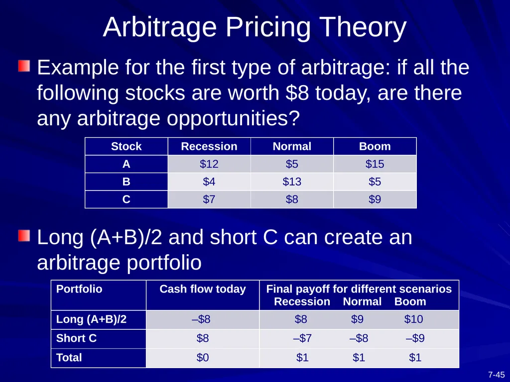
Arbitrage Pricing Theory Example for the first type of arbitrage: if all the following stocks are worth $8 today, are there any arbitrage opportunities?
Long (A+B)/2 and short C can create an arbitrage portfolio<br>
Long (A+B)/2 and short C can create an arbitrage portfolio<br>
46
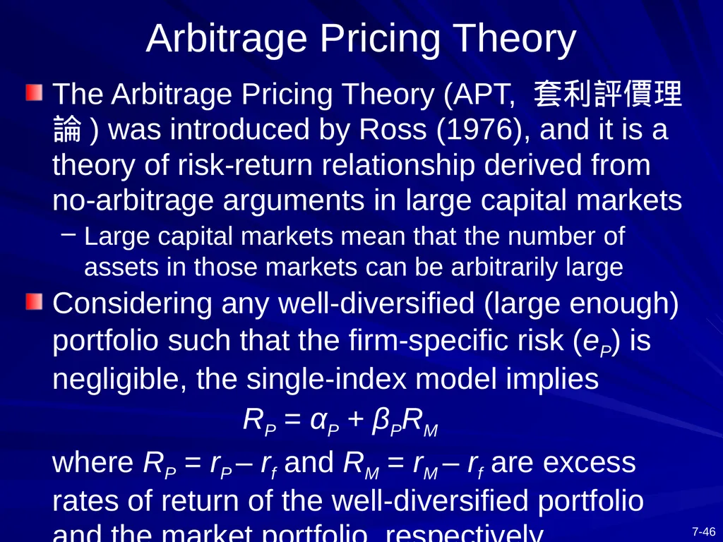
Arbitrage Pricing Theory The Arbitrage Pricing Theory (APT, 套利評價理論) was introduced by Ross (1976), and it is a theory of risk-return relationship derived from no-arbitrage arguments in large capital markets
Large capital markets mean that the number of assets in those markets can be arbitrarily large
Considering any well-diversified (large enough) portfolio such that the firm-specific risk (eP) is negligible, the single-index model implies
RP = αP + βPRM
where RP = rP – rf and RM = rM – rf are excess rates of return of the well-diversified portfolio and the market portfolio, respectively<br>
Large capital markets mean that the number of assets in those markets can be arbitrarily large
Considering any well-diversified (large enough) portfolio such that the firm-specific risk (eP) is negligible, the single-index model implies
RP = αP + βPRM
where RP = rP – rf and RM = rM – rf are excess rates of return of the well-diversified portfolio and the market portfolio, respectively<br>
47
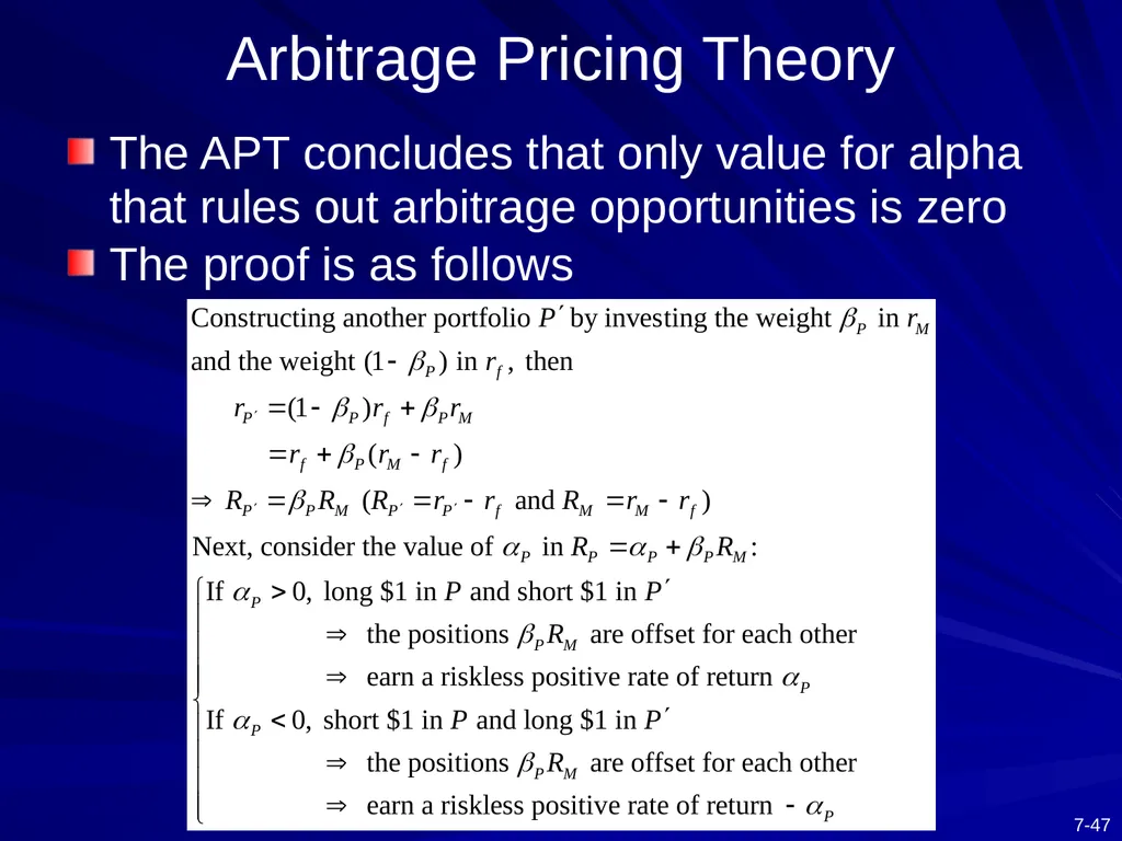
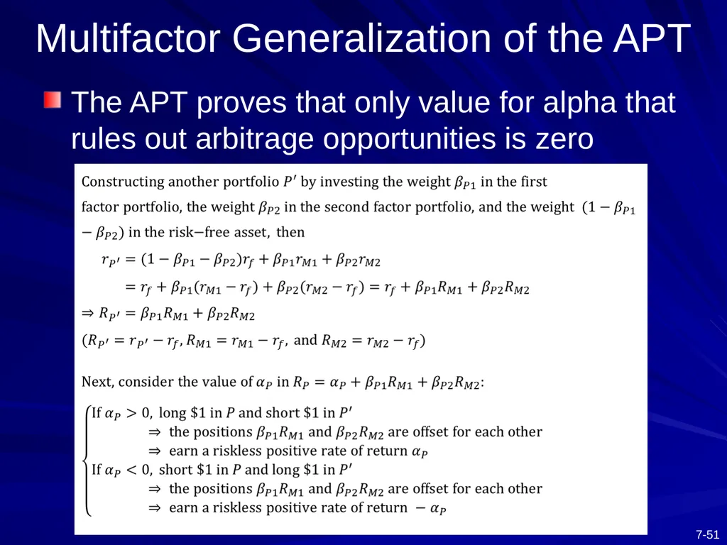
Arbitrage Pricing Theory The APT concludes that only value for alpha that rules out arbitrage opportunities is zero
The proof is as follows<br>
The proof is as follows<br>
48
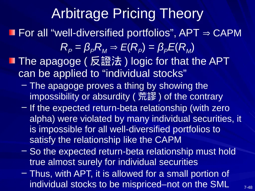
Arbitrage Pricing Theory For all “well-diversified portfolios”, APT CAPM
RP = βPRM E(RP) = βPE(RM)
The apagoge (反證法) logic for that the APT can be applied to “individual stocks”
The apagoge proves a thing by showing the impossibility or absurdity (荒謬) of the contrary
If the expected return-beta relationship (with zero alpha) were violated by many individual securities, it is impossible for all well-diversified portfolios to satisfy the relationship like the CAPM
So the expected return-beta relationship must hold true almost surely for individual securities
Thus, with APT, it is allowed for a small portion of individual stocks to be mispriced–not on the SML<br>
RP = βPRM E(RP) = βPE(RM)
The apagoge (反證法) logic for that the APT can be applied to “individual stocks”
The apagoge proves a thing by showing the impossibility or absurdity (荒謬) of the contrary
If the expected return-beta relationship (with zero alpha) were violated by many individual securities, it is impossible for all well-diversified portfolios to satisfy the relationship like the CAPM
So the expected return-beta relationship must hold true almost surely for individual securities
Thus, with APT, it is allowed for a small portion of individual stocks to be mispriced–not on the SML<br>
49
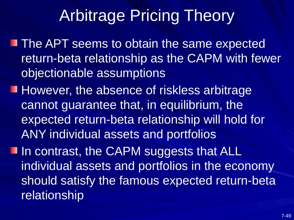
Arbitrage Pricing Theory The APT seems to obtain the same expected return-beta relationship as the CAPM with fewer objectionable assumptions
However, the absence of riskless arbitrage cannot guarantee that, in equilibrium, the expected return-beta relationship will hold for ANY individual assets and portfolios
In contrast, the CAPM suggests that ALL individual assets and portfolios in the economy should satisfy the famous expected return-beta relationship<br>
However, the absence of riskless arbitrage cannot guarantee that, in equilibrium, the expected return-beta relationship will hold for ANY individual assets and portfolios
In contrast, the CAPM suggests that ALL individual assets and portfolios in the economy should satisfy the famous expected return-beta relationship<br>
50
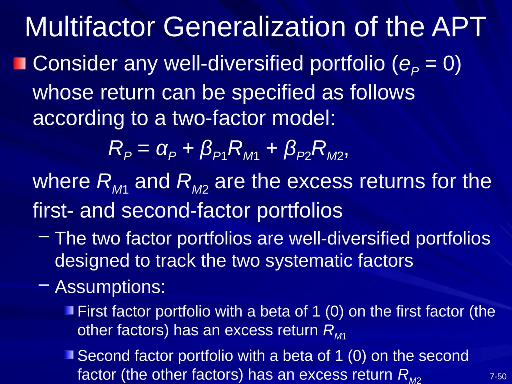
Multifactor Generalization of the APT Consider any well-diversified portfolio (eP = 0) whose return can be specified as follows according to a two-factor model:
RP = αP + βP1RM1 + βP2RM2,
where RM1 and RM2 are the excess returns for the first- and second-factor portfolios
The two factor portfolios are well-diversified portfolios designed to track the two systematic factors
Assumptions:
First factor portfolio with a beta of 1 (0) on the first factor (the other factors) has an excess return RM1
Second factor portfolio with a beta of 1 (0) on the second factor (the other factors) has an excess return RM2<br>
RP = αP + βP1RM1 + βP2RM2,
where RM1 and RM2 are the excess returns for the first- and second-factor portfolios
The two factor portfolios are well-diversified portfolios designed to track the two systematic factors
Assumptions:
First factor portfolio with a beta of 1 (0) on the first factor (the other factors) has an excess return RM1
Second factor portfolio with a beta of 1 (0) on the second factor (the other factors) has an excess return RM2<br>
51
The APT proves that only value for alpha that rules out arbitrage opportunities is zero Multifactor Generalization of the APT<br>
52
Multifactor Generalization of the APT Another way to explain that it does not need to calculate the excess return for rSMB and rHML<br>