
Chapter 11: The CAPM Corporate Finance Outline
YM
Published · 51 slides · 0 views

1 / 1



Description
Chapter 11: The CAPM Corporate Finance Outline Portfolio theory The CAPM (Capital Asset Pricing Model) Expected return with ex ante probabilities Investing usually needs to deal with uncertain outcomes. That is, the unrealized return can
Related Topics
Share
Embed code
Download this presentation From Below
"Chapter 11: The CAPM Corporate Finance Outline" is the property of its rightful owner. Permission is granted to download and print the materials on this website for personal, non-commercial use only, and to display it on your personal computer provided you do not modify the materials and that you retain all copyright notices contained in the materials. By downloading content from our website, you accept the terms of this agreement.
Presentation Transcript
01
Chapter 11: The CAPM Corporate Finance<br>
02
Outline Portfolio theory
The CAPM (Capital Asset Pricing Model)<br>
The CAPM (Capital Asset Pricing Model)<br>
03
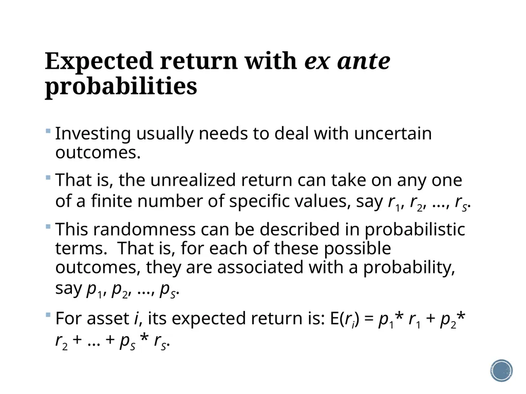
Expected return with ex ante probabilities Investing usually needs to deal with uncertain outcomes.
That is, the unrealized return can take on any one of a finite number of specific values, say r1, r2, …, rS.
This randomness can be described in probabilistic terms. That is, for each of these possible outcomes, they are associated with a probability, say p1, p2, …, pS.
For asset i, its expected return is: E(ri) = p1* r1 + p2* r2 + … + pS * rS.<br>
That is, the unrealized return can take on any one of a finite number of specific values, say r1, r2, …, rS.
This randomness can be described in probabilistic terms. That is, for each of these possible outcomes, they are associated with a probability, say p1, p2, …, pS.
For asset i, its expected return is: E(ri) = p1* r1 + p2* r2 + … + pS * rS.<br>
04
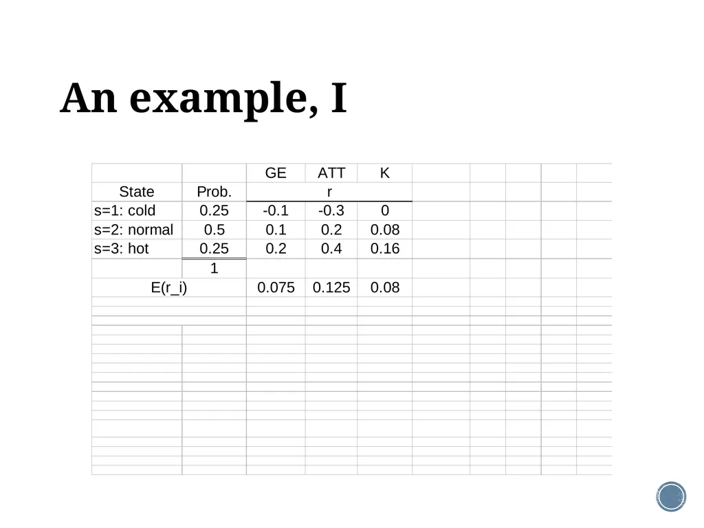
An example, I<br>
05
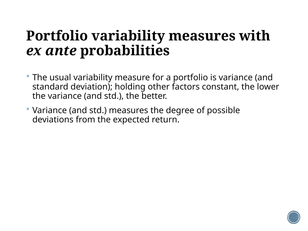
Portfolio variability measures with ex ante probabilities The usual variability measure for a portfolio is variance (and standard deviation); holding other factors constant, the lower the variance (and std.), the better.
Variance (and std.) measures the degree of possible deviations from the expected return.<br>
Variance (and std.) measures the degree of possible deviations from the expected return.<br>
06
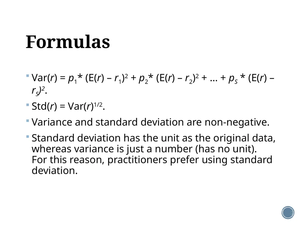
Formulas Var(r) = p1* (E(r) – r1)2 + p2* (E(r) – r2)2 + … + pS * (E(r) – rS)2.
Std(r) = Var(r)1/2.
Variance and standard deviation are non-negative.
Standard deviation has the unit as the original data, whereas variance is just a number (has no unit). For this reason, practitioners prefer using standard deviation.<br>
Std(r) = Var(r)1/2.
Variance and standard deviation are non-negative.
Standard deviation has the unit as the original data, whereas variance is just a number (has no unit). For this reason, practitioners prefer using standard deviation.<br>
07
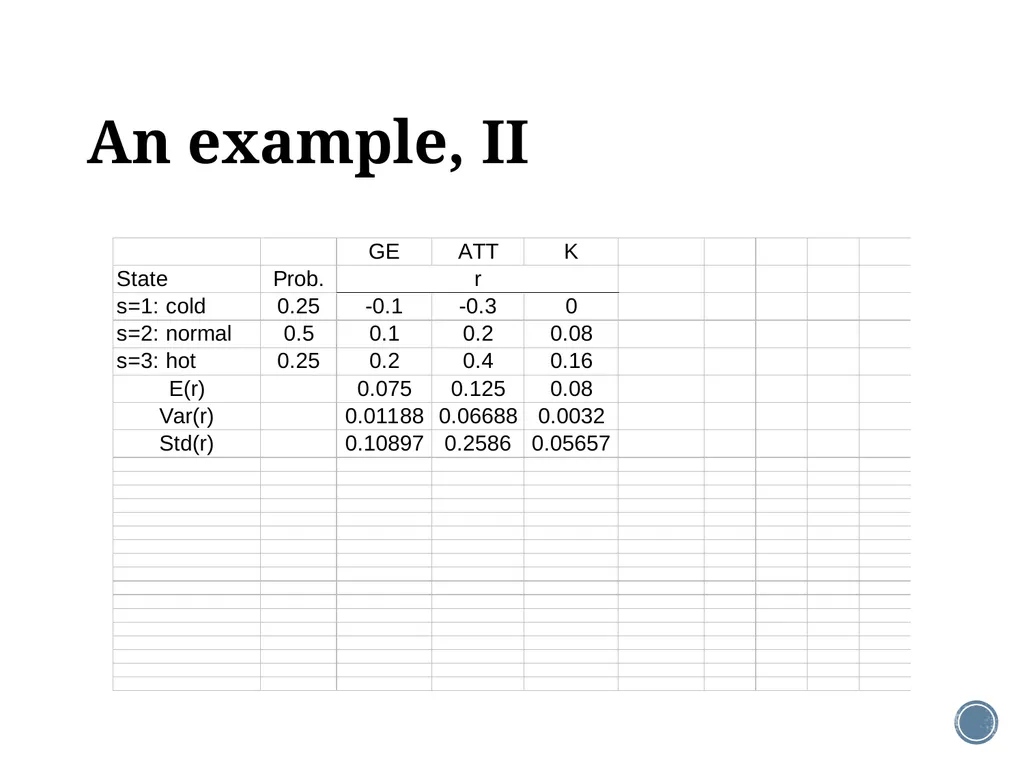
An example, II<br>
08
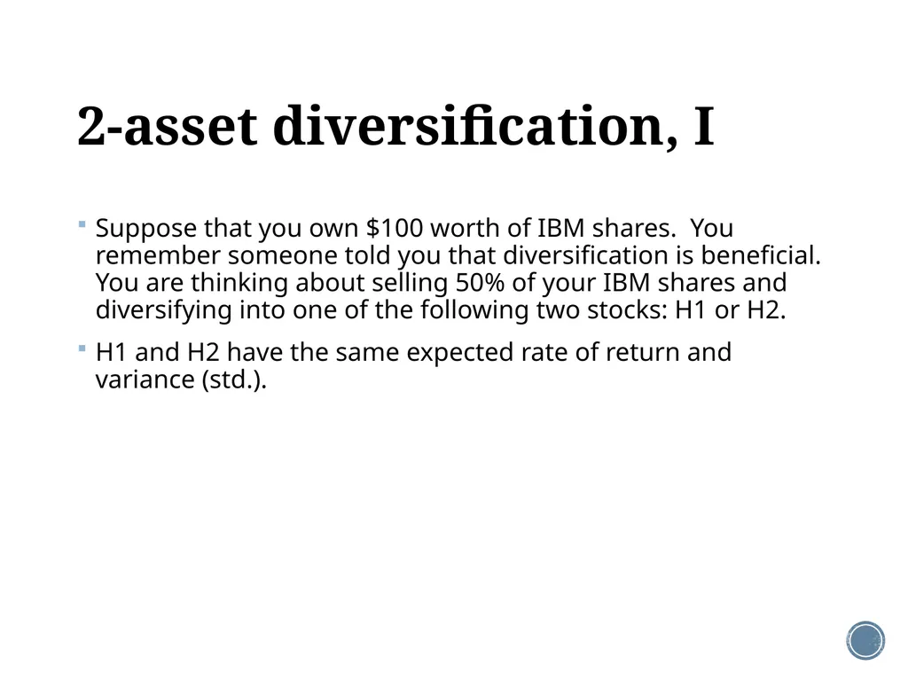
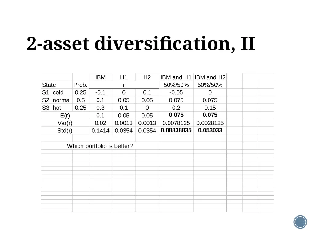
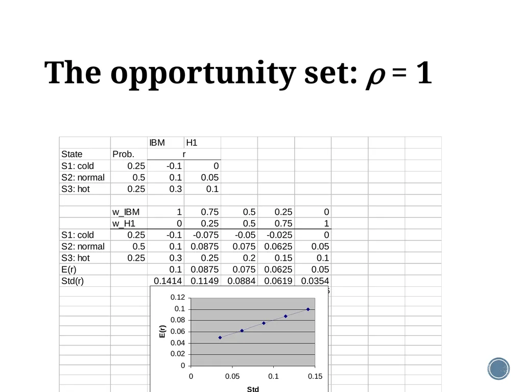
2-asset diversification, I Suppose that you own $100 worth of IBM shares. You remember someone told you that diversification is beneficial. You are thinking about selling 50% of your IBM shares and diversifying into one of the following two stocks: H1 or H2.
H1 and H2 have the same expected rate of return and variance (std.).<br>
H1 and H2 have the same expected rate of return and variance (std.).<br>
09
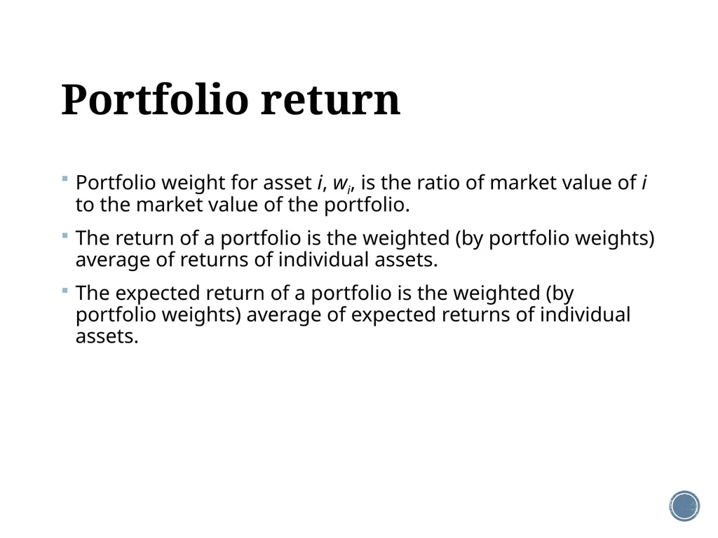
Portfolio return Portfolio weight for asset i, wi, is the ratio of market value of i to the market value of the portfolio.
The return of a portfolio is the weighted (by portfolio weights) average of returns of individual assets.
The expected return of a portfolio is the weighted (by portfolio weights) average of expected returns of individual assets.<br>
The return of a portfolio is the weighted (by portfolio weights) average of returns of individual assets.
The expected return of a portfolio is the weighted (by portfolio weights) average of expected returns of individual assets.<br>
10
2-asset diversification, II<br>
11
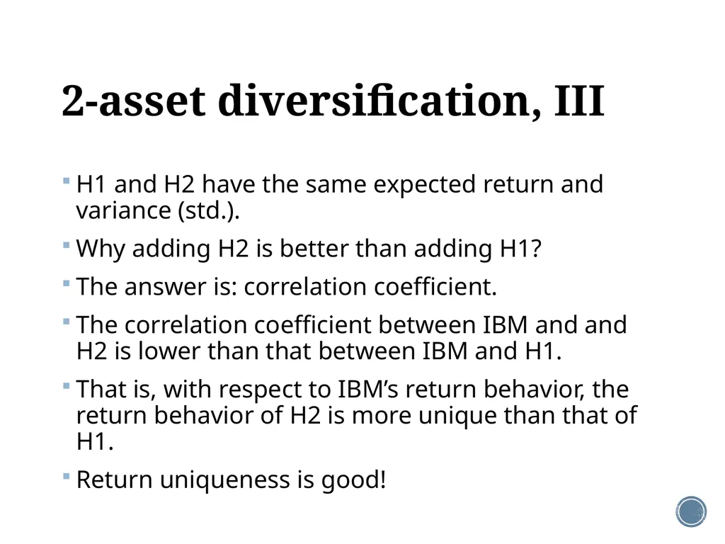
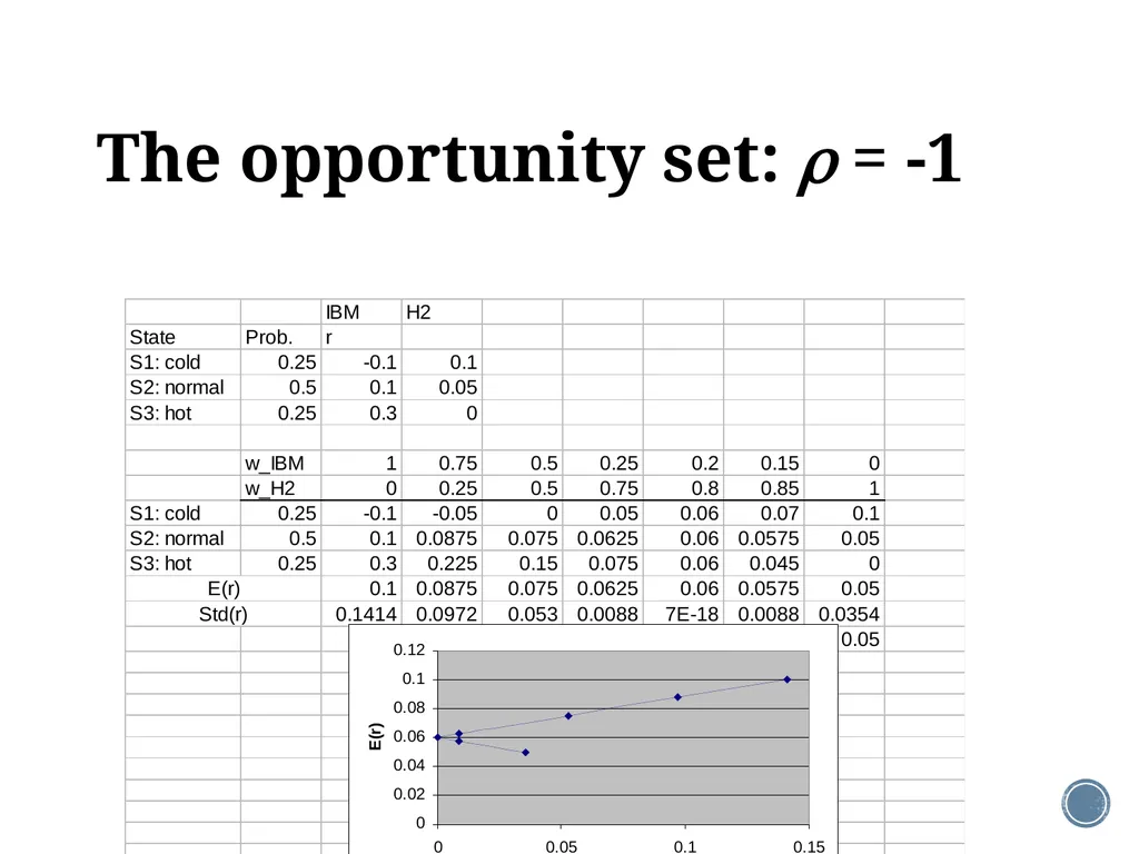
2-asset diversification, III H1 and H2 have the same expected return and variance (std.).
Why adding H2 is better than adding H1?
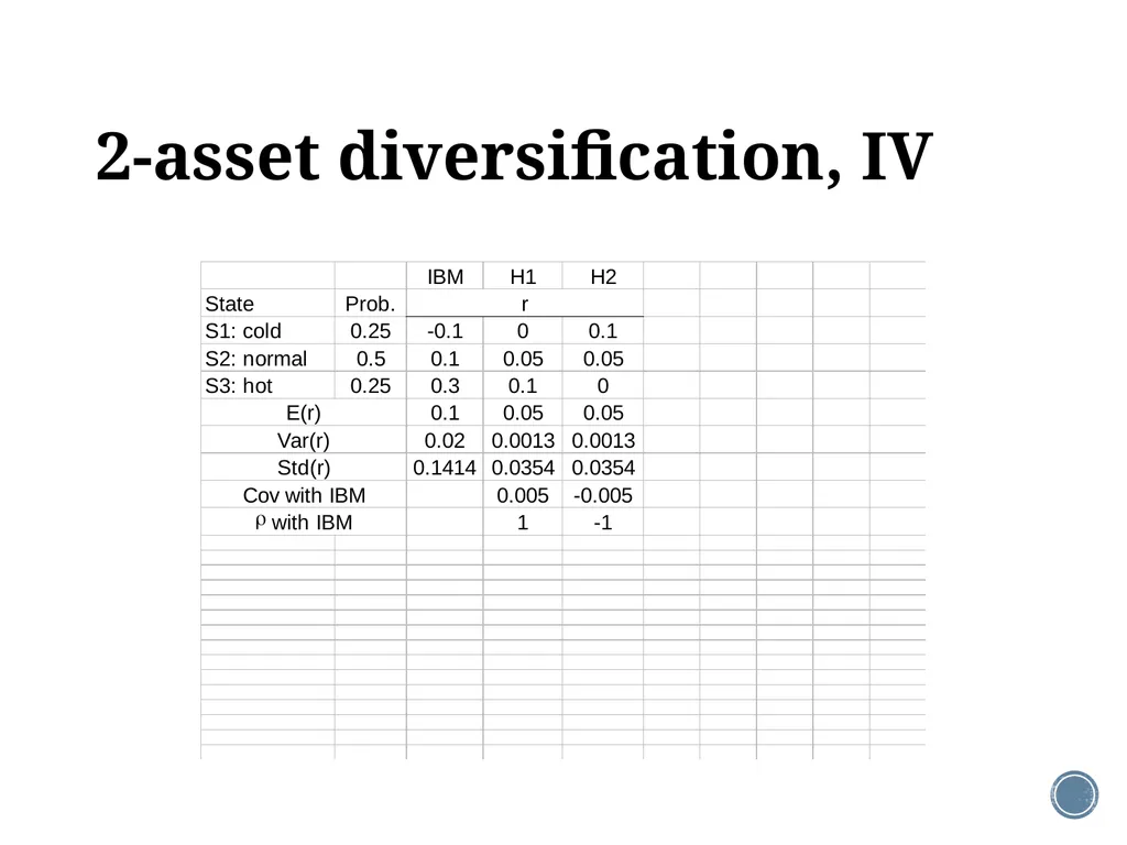
The answer is: correlation coefficient.
The correlation coefficient between IBM and and H2 is lower than that between IBM and H1.
That is, with respect to IBM’s return behavior, the return behavior of H2 is more unique than that of H1.
Return uniqueness is good!<br>
Why adding H2 is better than adding H1?
The answer is: correlation coefficient.
The correlation coefficient between IBM and and H2 is lower than that between IBM and H1.
That is, with respect to IBM’s return behavior, the return behavior of H2 is more unique than that of H1.
Return uniqueness is good!<br>
12
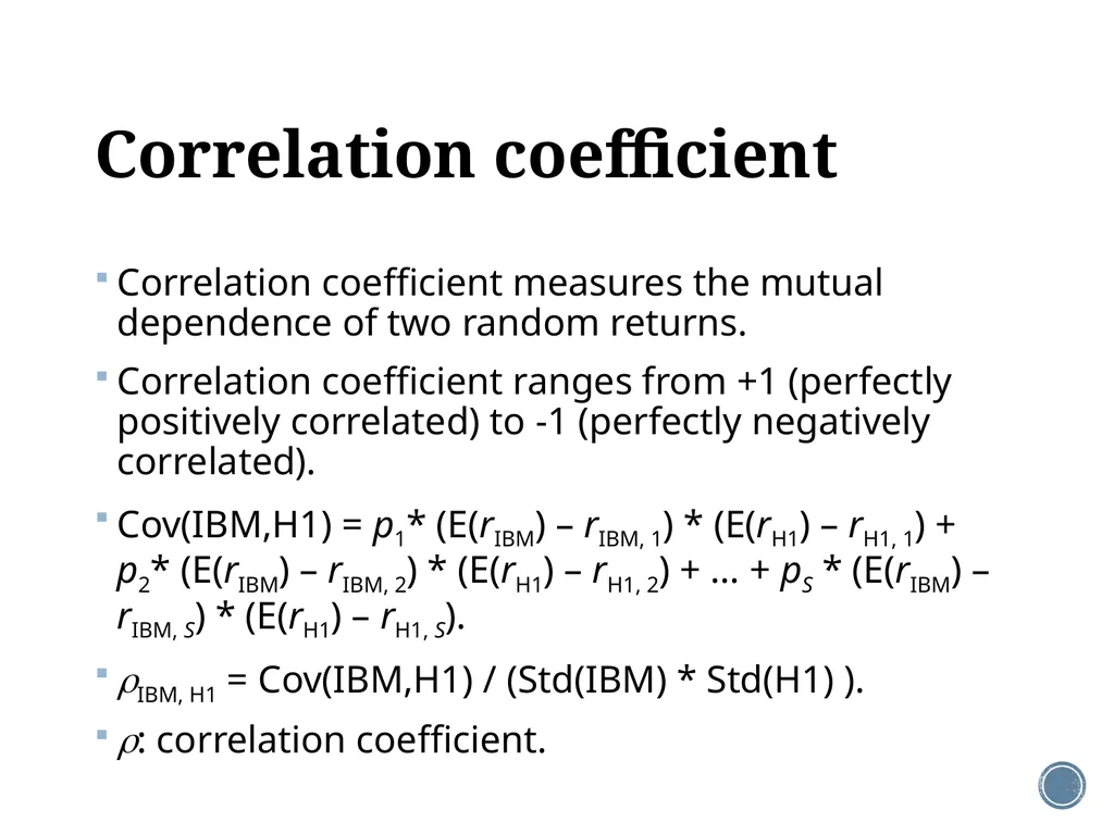
Correlation coefficient Correlation coefficient measures the mutual dependence of two random returns.
Correlation coefficient ranges from +1 (perfectly positively correlated) to -1 (perfectly negatively correlated).
Cov(IBM,H1) = p1* (E(rIBM) – rIBM, 1) * (E(rH1) – rH1, 1) + p2* (E(rIBM) – rIBM, 2) * (E(rH1) – rH1, 2) + … + pS * (E(rIBM) – rIBM, S) * (E(rH1) – rH1, S).
IBM, H1 = Cov(IBM,H1) / (Std(IBM) * Std(H1) ).
: correlation coefficient.<br>
Correlation coefficient ranges from +1 (perfectly positively correlated) to -1 (perfectly negatively correlated).
Cov(IBM,H1) = p1* (E(rIBM) – rIBM, 1) * (E(rH1) – rH1, 1) + p2* (E(rIBM) – rIBM, 2) * (E(rH1) – rH1, 2) + … + pS * (E(rIBM) – rIBM, S) * (E(rH1) – rH1, S).
IBM, H1 = Cov(IBM,H1) / (Std(IBM) * Std(H1) ).
: correlation coefficient.<br>
13
2-asset diversification, IV<br>
14
The opportunity set: = 1<br>
15
The opportunity set: = -1<br>
16
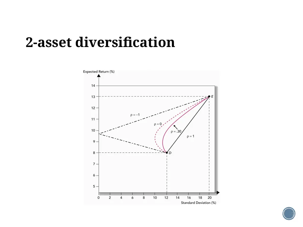
2-asset diversification<br>
17
So, these are what we have so far: The shape of the combinations of 2 assets is like a rubber band.
With a low correlation coefficient, you can pull the rubber band further to the left, which is good.
Holding other factors constant, the lower the correlation coefficient, the better.
Again, return uniqueness is healthy!<br>
With a low correlation coefficient, you can pull the rubber band further to the left, which is good.
Holding other factors constant, the lower the correlation coefficient, the better.
Again, return uniqueness is healthy!<br>
18
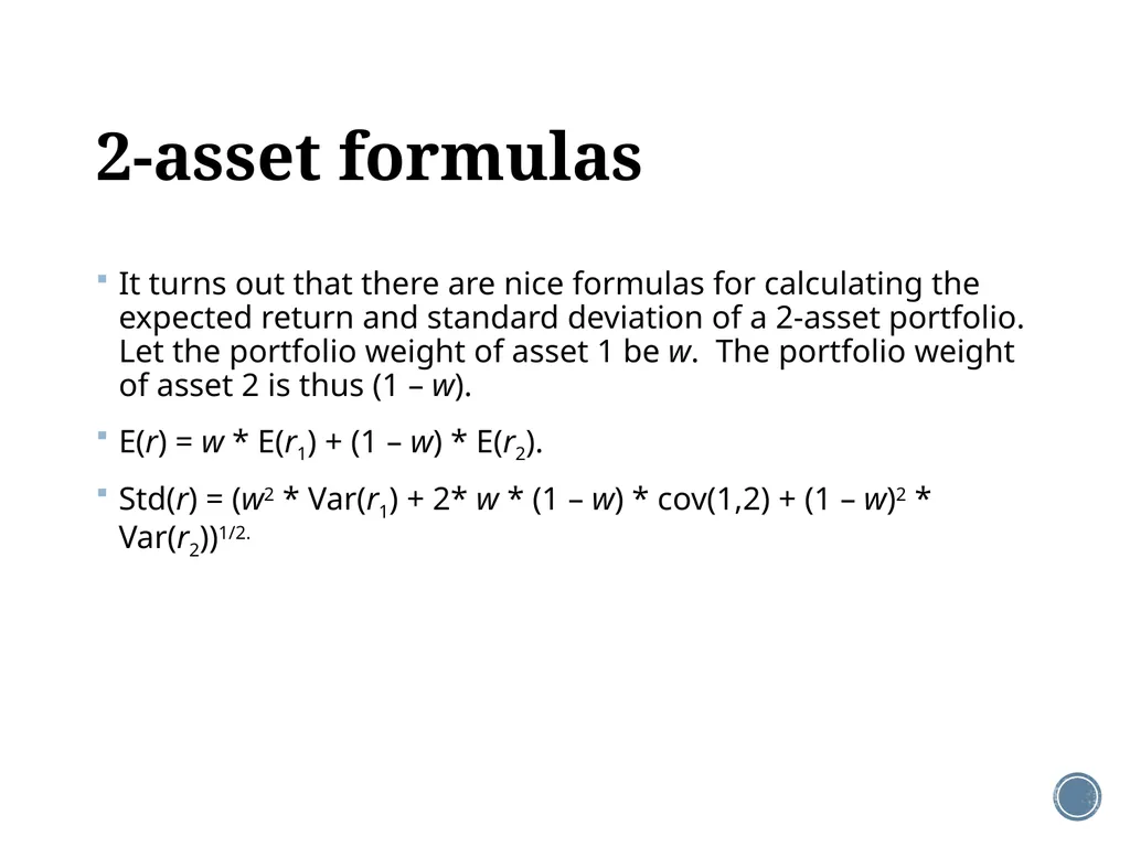
2-asset formulas It turns out that there are nice formulas for calculating the expected return and standard deviation of a 2-asset portfolio. Let the portfolio weight of asset 1 be w. The portfolio weight of asset 2 is thus (1 – w).
E(r) = w * E(r1) + (1 – w) * E(r2).
Std(r) = (w2 * Var(r1) + 2* w * (1 – w) * cov(1,2) + (1 – w)2 * Var(r2))1/2.<br>
E(r) = w * E(r1) + (1 – w) * E(r2).
Std(r) = (w2 * Var(r1) + 2* w * (1 – w) * cov(1,2) + (1 – w)2 * Var(r2))1/2.<br>
19
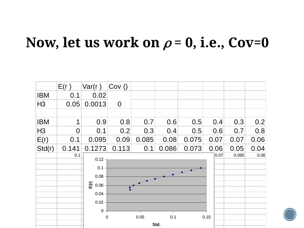
Now, let us work on = 0, i.e., Cov=0<br>
20
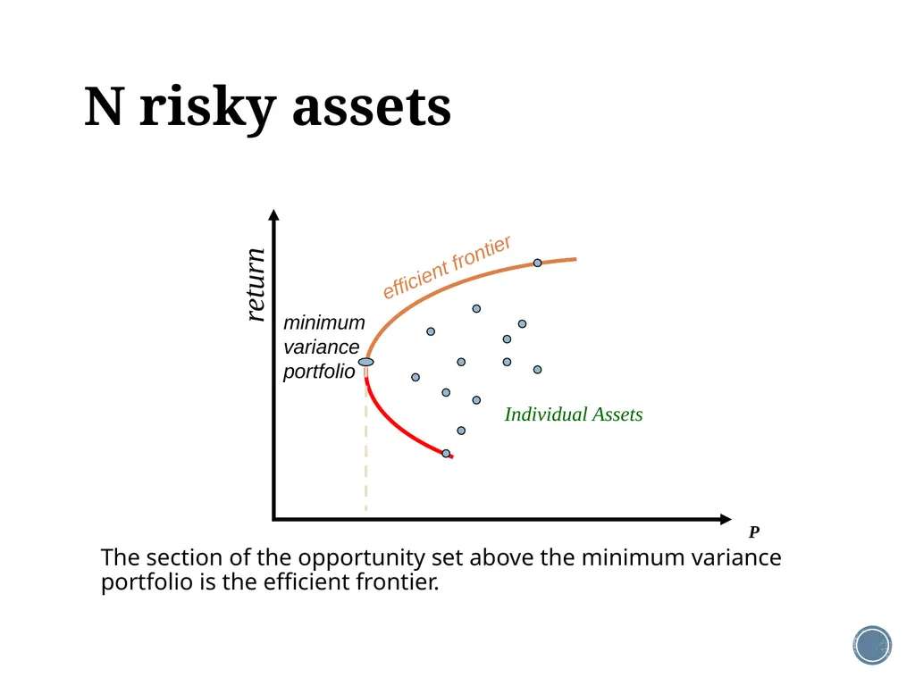
N risky assets The section of the opportunity set above the minimum variance portfolio is the efficient frontier. return P minimum variance portfolio efficient frontier Individual Assets<br>
21
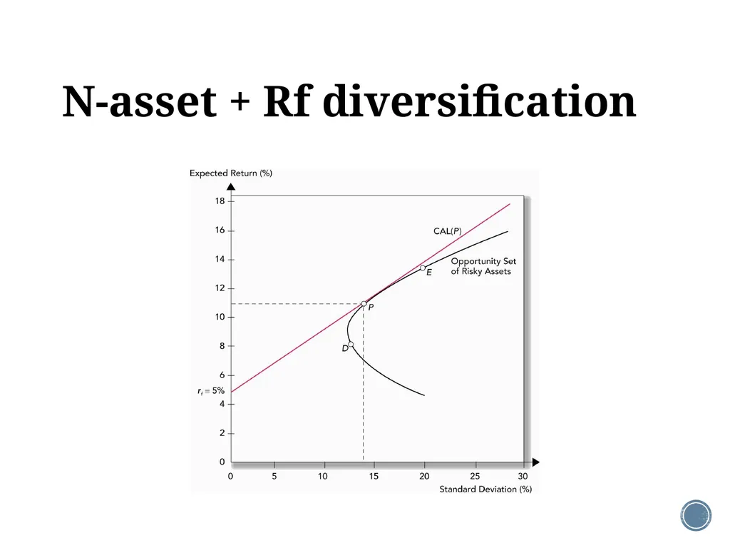
N-asset + Rf diversification<br>
22
Selecting an optimal portfolio from N>2 assets The upper part of the bullet-shape solid line is the efficient frontier (EF): the set of portfolios that have the highest expected return given a particular level of risk (std.).
Given the EF, selecting an optimal portfolio for an investor who are allowed to invest in a combination of N risky assets is rather straightforward.
One way is to ask the investor about the comfortable level of standard deviation (risk tolerance), say 20%. Then, corresponding to that level of std., we find the optimal portfolio on the EF, say the portfolio E shown in the previous figure.
CAL (capital allocation line): the set of feasible expected return and standard deviation pairs of all portfolios resulting from combining the risk-free asset and a risky portfolio.<br>
Given the EF, selecting an optimal portfolio for an investor who are allowed to invest in a combination of N risky assets is rather straightforward.
One way is to ask the investor about the comfortable level of standard deviation (risk tolerance), say 20%. Then, corresponding to that level of std., we find the optimal portfolio on the EF, say the portfolio E shown in the previous figure.
CAL (capital allocation line): the set of feasible expected return and standard deviation pairs of all portfolios resulting from combining the risk-free asset and a risky portfolio.<br>
23
What if one can invest in the risk-free asset? If we add the risk-free asset to N risky assets, we can enhance the efficient frontier (EF) to the red line shown in the previous figure, i.e., the straight line that passes through the risk-free asset and the tangent point of the efficient frontier (EF).
Let us called this straight line “enhanced efficient frontier” (EEF).<br>
Let us called this straight line “enhanced efficient frontier” (EEF).<br>
24
Enhanced efficient frontier (EEF) With the risk-free asset, EEF will be of interest to rational investors who do not like standard deviation and like expected return.
Why EEF pass through the tangent point? The reason is that this line has the highest slope; that is, given one unit of std. (variance), the associated expected return is the highest.
Why EEF is a straight line? This is because the risk-free asset, by definition, has zero variance (std.) and zero covariance with any risky asset.<br>
Why EEF pass through the tangent point? The reason is that this line has the highest slope; that is, given one unit of std. (variance), the associated expected return is the highest.
Why EEF is a straight line? This is because the risk-free asset, by definition, has zero variance (std.) and zero covariance with any risky asset.<br>
25
Separation, I When the risk-free asset is available, any efficient portfolio (any point on the EEF) can be expressed as a combination of the tangent portfolio and the risk-free asset.
Implication: in terms of choosing risky investments, there will be no need for anyone to purchase individual stocks separately or to purchase other risky portfolios; the tangent portfolio is enough.<br>
Implication: in terms of choosing risky investments, there will be no need for anyone to purchase individual stocks separately or to purchase other risky portfolios; the tangent portfolio is enough.<br>
26
Separation, II Once an investor makes the above “investment” decision, i.e., finding the tangent portfolio, the remaining task will be a “financing” decision. That is, including the risk-free asset (either long or short) such that the resulting efficient portfolio meets the investor’s risk tolerance.
The “financing” decision is independent (separation) of the “investment” decision.<br>
The “financing” decision is independent (separation) of the “investment” decision.<br>
27
EEF vs. EF EEF is almost surely better off than EF, except for the tangent portfolio.
In other words, adding the risk-free asset (either a long or short position) into a risky portfolio is almost surely beneficial.
Why? [hint: correlation coefficient].<br>
In other words, adding the risk-free asset (either a long or short position) into a risky portfolio is almost surely beneficial.
Why? [hint: correlation coefficient].<br>
28
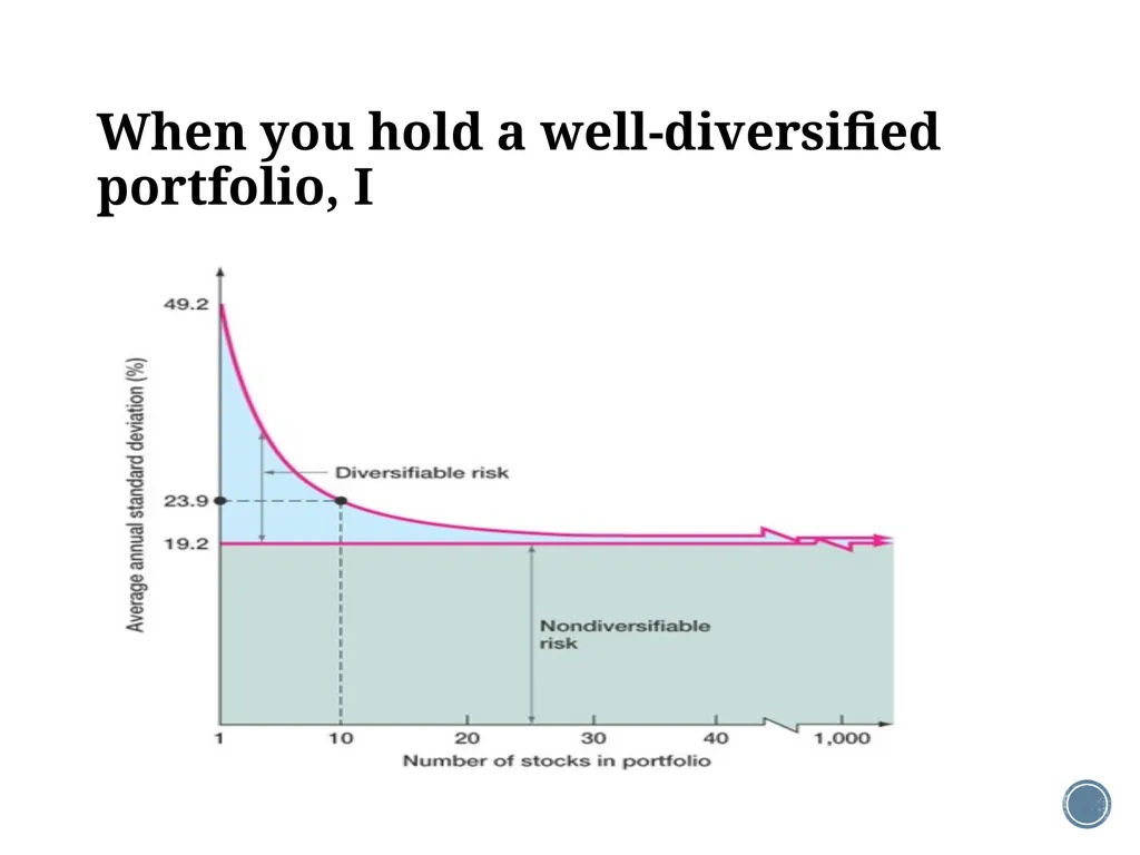
When you hold a well-diversified portfolio, I<br>
29
When you hold a well-diversified portfolio, II When one holds a well-diversified portfolio, the so called diversifiable (unsystematic, or idiosyncratic) risk disappears.
Unsystematic risk: the type of risk that affects a limited number of assets.
Because unsystematic risk can be easily diversified away by holding a large number of assets, rational investors would not want unsystematic risk in their portfolios.
Thus, this type of risk does not require risk premium.
Risk premium: the difference between expected return and the risk-free rate.<br>
Unsystematic risk: the type of risk that affects a limited number of assets.
Because unsystematic risk can be easily diversified away by holding a large number of assets, rational investors would not want unsystematic risk in their portfolios.
Thus, this type of risk does not require risk premium.
Risk premium: the difference between expected return and the risk-free rate.<br>
30
When you hold a well-diversified portfolio, III Even when one holds a well-diversified portfolio, the so called un-diversifiable ( or systematic) risk will not be reduced.
Systematic risk: the type of (market-wide) risk that affects a large number of assets.
Because systematic risk cannot be diversified away, investors need to live with it (monkey on the shoulder) when investing in risky securities.
Thus, this type of risk does require risk premium.<br>
Systematic risk: the type of (market-wide) risk that affects a large number of assets.
Because systematic risk cannot be diversified away, investors need to live with it (monkey on the shoulder) when investing in risky securities.
Thus, this type of risk does require risk premium.<br>
31
Beta as a measure of systematic risk Systematic risk matters!
We use the beta coefficient to measure systematic risk.
Beta: a measure of the responsiveness of a security to movements in the market. Betai = Cov (i, m) / Var (m).<br>
We use the beta coefficient to measure systematic risk.
Beta: a measure of the responsiveness of a security to movements in the market. Betai = Cov (i, m) / Var (m).<br>
32
More about beta What does beta tell us?
A beta < 1 implies the asset has less systematic risk than the overall market.
A beta > 1 implies the asset has more systematic risk than the overall market.
The overall market has a beta of 1.
The beta of the risk-free asset is 0. Why?<br>
A beta < 1 implies the asset has less systematic risk than the overall market.
A beta > 1 implies the asset has more systematic risk than the overall market.
The overall market has a beta of 1.
The beta of the risk-free asset is 0. Why?<br>
33
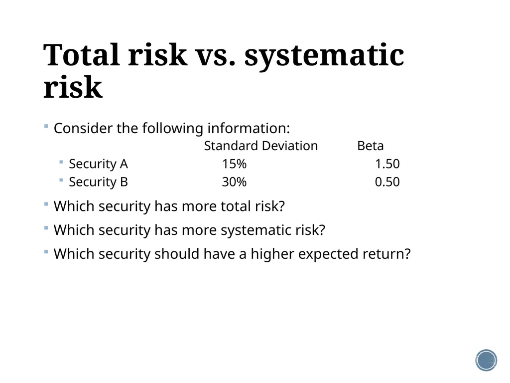
Total risk vs. systematic risk Consider the following information:
Standard Deviation Beta
Security A 15% 1.50
Security B 30% 0.50
Which security has more total risk?
Which security has more systematic risk?
Which security should have a higher expected return?<br>
Standard Deviation Beta
Security A 15% 1.50
Security B 30% 0.50
Which security has more total risk?
Which security has more systematic risk?
Which security should have a higher expected return?<br>
34
Risk, again For a portfolio, we care about variance and standard deviation.
But this risk concept at portfolio level does not automatically carry forward to individual security level.
For a security, we care about beta.
The reason is that variances and standard deviations do not add up. They may cancel one another out.<br>
But this risk concept at portfolio level does not automatically carry forward to individual security level.
For a security, we care about beta.
The reason is that variances and standard deviations do not add up. They may cancel one another out.<br>
35
Beta and risk premium So far, we know that beta is a measure of systematic risk, and bearing systematic risk requires compensation in the form of extra return (expected return).
Thus, the higher the beta, the greater the risk premium.
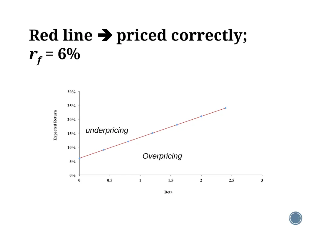
This relationship is depicted in the following figure.<br>
Thus, the higher the beta, the greater the risk premium.
This relationship is depicted in the following figure.<br>
36
Red line priced correctly;
rf = 6% Overpricing underpricing<br>
37
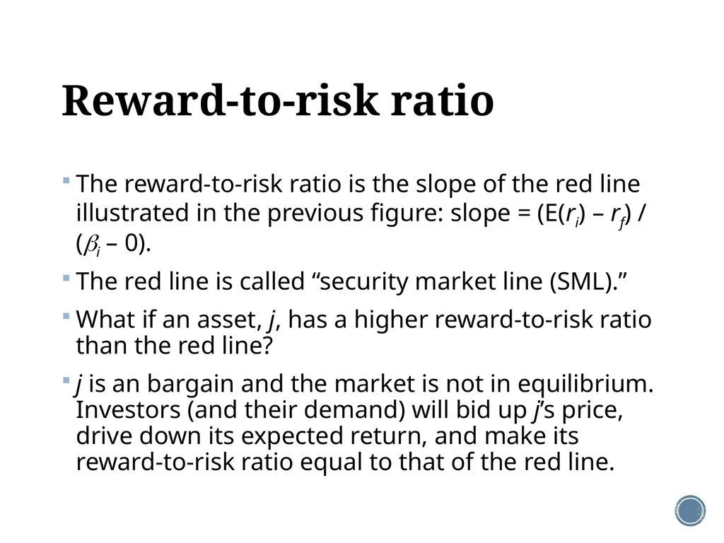
Reward-to-risk ratio The reward-to-risk ratio is the slope of the red line illustrated in the previous figure: slope = (E(ri) – rf) / (i – 0).
The red line is called “security market line (SML).”
What if an asset, j, has a higher reward-to-risk ratio than the red line?
j is an bargain and the market is not in equilibrium. Investors (and their demand) will bid up j’s price, drive down its expected return, and make its reward-to-risk ratio equal to that of the red line.<br>
The red line is called “security market line (SML).”
What if an asset, j, has a higher reward-to-risk ratio than the red line?
j is an bargain and the market is not in equilibrium. Investors (and their demand) will bid up j’s price, drive down its expected return, and make its reward-to-risk ratio equal to that of the red line.<br>
38
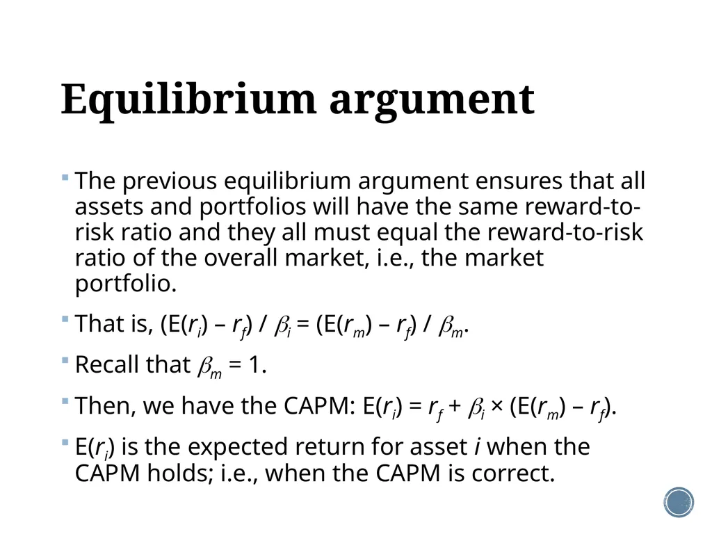
Equilibrium argument The previous equilibrium argument ensures that all assets and portfolios will have the same reward-to-risk ratio and they all must equal the reward-to-risk ratio of the overall market, i.e., the market portfolio.
That is, (E(ri) – rf) / i = (E(rm) – rf) / m.
Recall that m = 1.
Then, we have the CAPM: E(ri) = rf + i × (E(rm) – rf).
E(ri) is the expected return for asset i when the CAPM holds; i.e., when the CAPM is correct.<br>
That is, (E(ri) – rf) / i = (E(rm) – rf) / m.
Recall that m = 1.
Then, we have the CAPM: E(ri) = rf + i × (E(rm) – rf).
E(ri) is the expected return for asset i when the CAPM holds; i.e., when the CAPM is correct.<br>
39
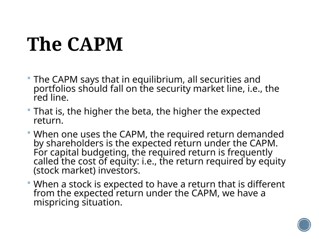
The CAPM The CAPM says that in equilibrium, all securities and portfolios should fall on the security market line, i.e., the red line.
That is, the higher the beta, the higher the expected return.
When one uses the CAPM, the required return demanded by shareholders is the expected return under the CAPM. For capital budgeting, the required return is frequently called the cost of equity: i.e., the return required by equity (stock market) investors.
When a stock is expected to have a return that is different from the expected return under the CAPM, we have a mispricing situation.<br>
That is, the higher the beta, the higher the expected return.
When one uses the CAPM, the required return demanded by shareholders is the expected return under the CAPM. For capital budgeting, the required return is frequently called the cost of equity: i.e., the return required by equity (stock market) investors.
When a stock is expected to have a return that is different from the expected return under the CAPM, we have a mispricing situation.<br>
40
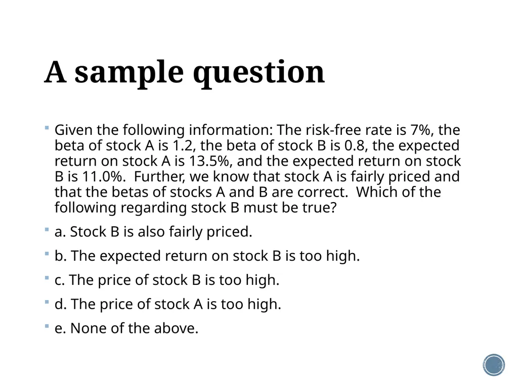
A sample question Given the following information: The risk-free rate is 7%, the beta of stock A is 1.2, the beta of stock B is 0.8, the expected return on stock A is 13.5%, and the expected return on stock B is 11.0%. Further, we know that stock A is fairly priced and that the betas of stocks A and B are correct. Which of the following regarding stock B must be true?
a. Stock B is also fairly priced.
b. The expected return on stock B is too high.
c. The price of stock B is too high.
d. The price of stock A is too high.
e. None of the above.<br>
a. Stock B is also fairly priced.
b. The expected return on stock B is too high.
c. The price of stock B is too high.
d. The price of stock A is too high.
e. None of the above.<br>
41
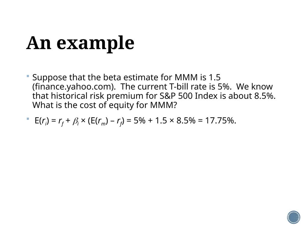
An example Suppose that the beta estimate for MMM is 1.5 (finance.yahoo.com). The current T-bill rate is 5%. We know that historical risk premium for S&P 500 Index is about 8.5%. What is the cost of equity for MMM?
E(ri) = rf + i × (E(rm) – rf) = 5% + 1.5 × 8.5% = 17.75%.<br>
E(ri) = rf + i × (E(rm) – rf) = 5% + 1.5 × 8.5% = 17.75%.<br>
42
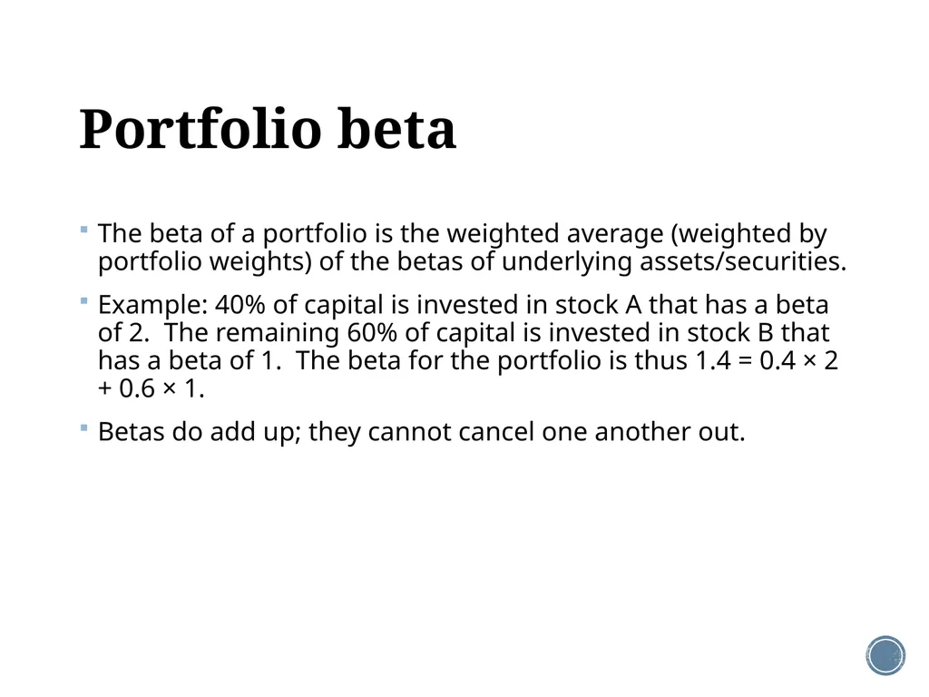
Portfolio beta The beta of a portfolio is the weighted average (weighted by portfolio weights) of the betas of underlying assets/securities.
Example: 40% of capital is invested in stock A that has a beta of 2. The remaining 60% of capital is invested in stock B that has a beta of 1. The beta for the portfolio is thus 1.4 = 0.4 × 2 + 0.6 × 1.
Betas do add up; they cannot cancel one another out.<br>
Example: 40% of capital is invested in stock A that has a beta of 2. The remaining 60% of capital is invested in stock B that has a beta of 1. The beta for the portfolio is thus 1.4 = 0.4 × 2 + 0.6 × 1.
Betas do add up; they cannot cancel one another out.<br>
43
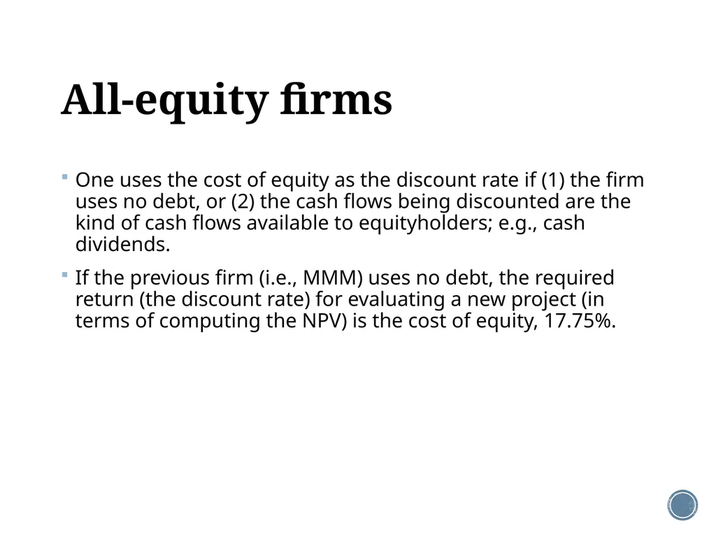
All-equity firms One uses the cost of equity as the discount rate if (1) the firm uses no debt, or (2) the cash flows being discounted are the kind of cash flows available to equityholders; e.g., cash dividends.
If the previous firm (i.e., MMM) uses no debt, the required return (the discount rate) for evaluating a new project (in terms of computing the NPV) is the cost of equity, 17.75%.<br>
If the previous firm (i.e., MMM) uses no debt, the required return (the discount rate) for evaluating a new project (in terms of computing the NPV) is the cost of equity, 17.75%.<br>
44
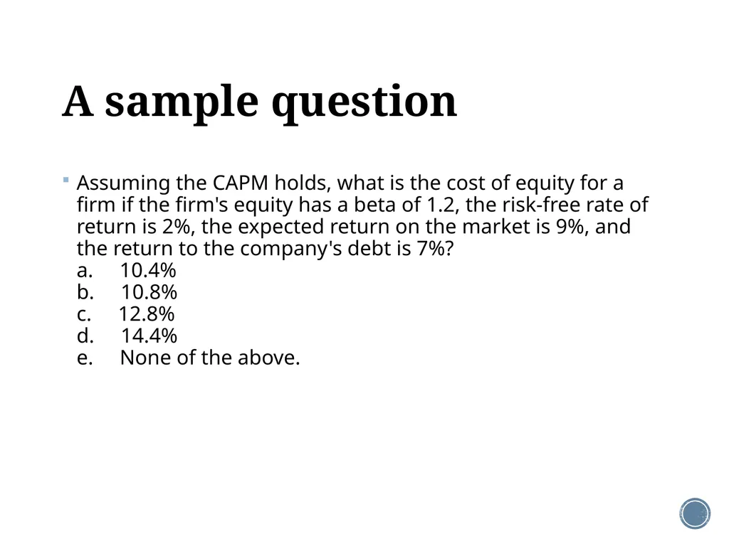
A sample question Assuming the CAPM holds, what is the cost of equity for a firm if the firm's equity has a beta of 1.2, the risk-free rate of return is 2%, the expected return on the market is 9%, and the return to the company's debt is 7%?
a. 10.4%
b. 10.8%
c. 12.8%
d. 14.4%
e. None of the above.<br>
45
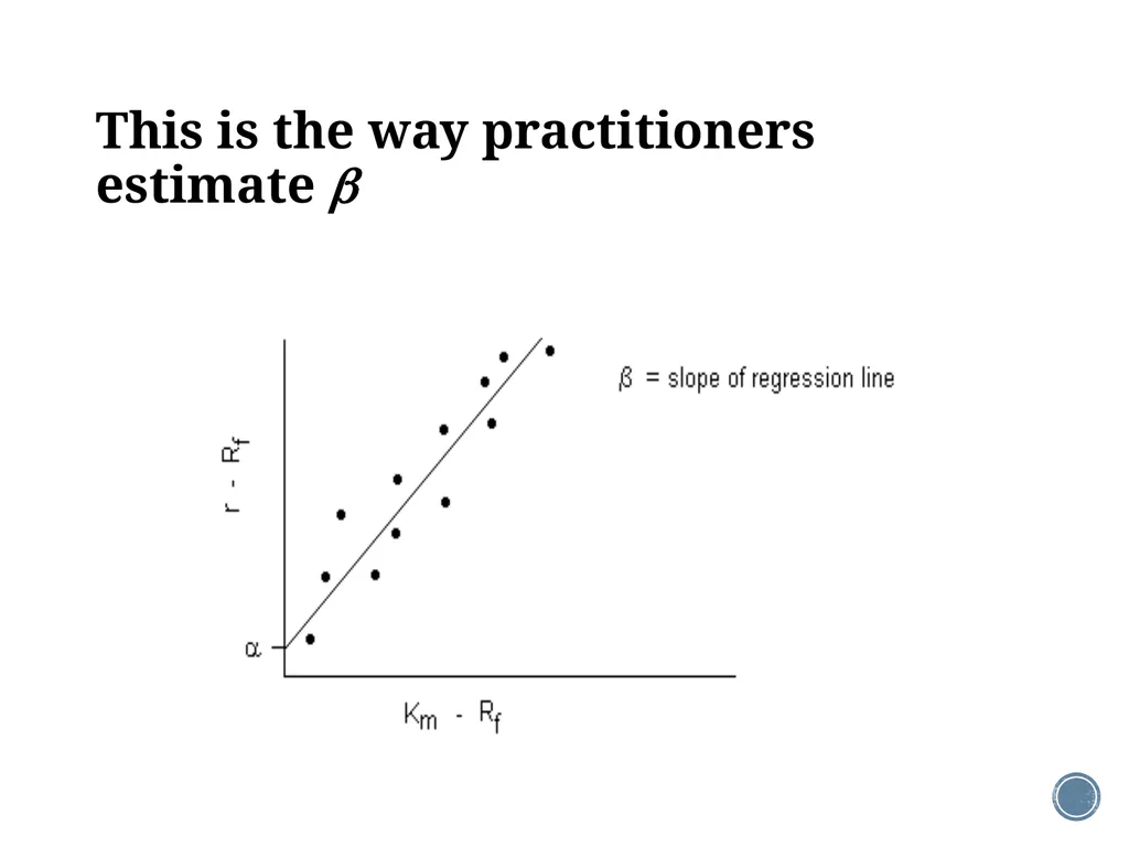
This is the way practitioners estimate <br>
46
Characteristic line The previous regression line is called the characteristic line.
The slope of the characteristic line is an estimate of .
The intercept term estimate is called “alpha.”<br>
The slope of the characteristic line is an estimate of .
The intercept term estimate is called “alpha.”<br>
47
Is the CAPM a good model? It is a beautiful model.
It does not have desirable empirical properties.
In recent years, more and more people would like to see a better way of estimating the cost of equity.
Possible directions: multi-factor models? real-option-based models?<br>
It does not have desirable empirical properties.
In recent years, more and more people would like to see a better way of estimating the cost of equity.
Possible directions: multi-factor models? real-option-based models?<br>
48
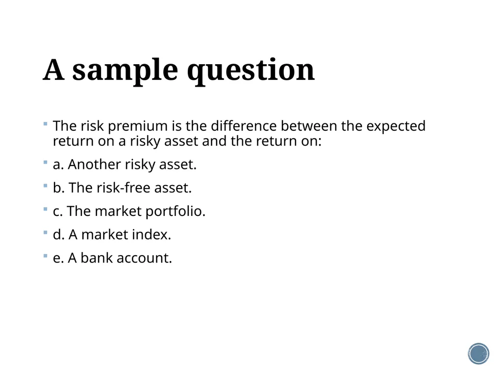
A sample question The risk premium is the difference between the expected return on a risky asset and the return on:
a. Another risky asset.
b. The risk-free asset.
c. The market portfolio.
d. A market index.
e. A bank account.<br>
a. Another risky asset.
b. The risk-free asset.
c. The market portfolio.
d. A market index.
e. A bank account.<br>
49
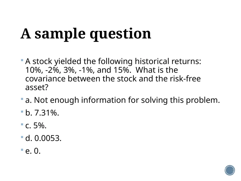
A sample question A stock yielded the following historical returns: 10%, -2%, 3%, -1%, and 15%. What is the covariance between the stock and the risk-free asset?
a. Not enough information for solving this problem.
b. 7.31%.
c. 5%.
d. 0.0053.
e. 0.<br>
a. Not enough information for solving this problem.
b. 7.31%.
c. 5%.
d. 0.0053.
e. 0.<br>
50
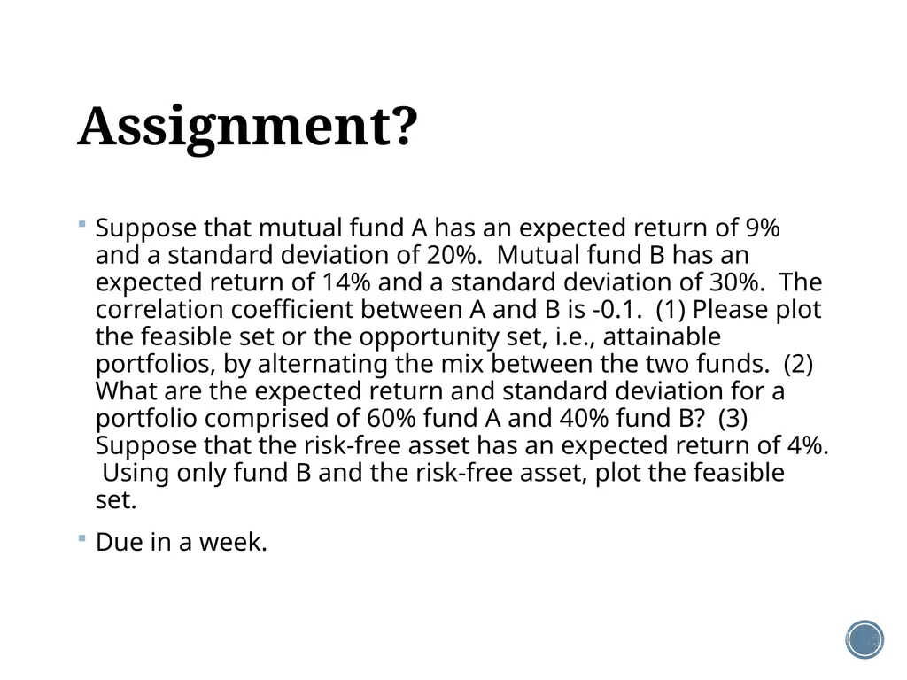
Assignment? Suppose that mutual fund A has an expected return of 9% and a standard deviation of 20%. Mutual fund B has an expected return of 14% and a standard deviation of 30%. The correlation coefficient between A and B is -0.1. (1) Please plot the feasible set or the opportunity set, i.e., attainable portfolios, by alternating the mix between the two funds. (2) What are the expected return and standard deviation for a portfolio comprised of 60% fund A and 40% fund B? (3) Suppose that the risk-free asset has an expected return of 4%. Using only fund B and the risk-free asset, plot the feasible set.
Due in a week.<br>
Due in a week.<br>
51
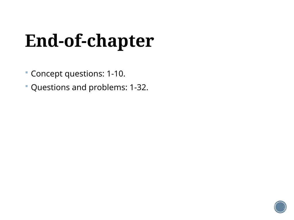
End-of-chapter Concept questions: 1-10.
Questions and problems: 1-32.<br>
Questions and problems: 1-32.<br>