
Chapter 3 Comparing Disease Frequencies Our
DJ
Published · 60 slides · 0 views
1 / 1

Description
Chapter 3 Comparing Disease Frequencies Our Touchstone Epidemiology is the study of the distribution and determinants of disease frequency in human populations and the application of this study to control health problems. Last Weeks
Related Topics
Share
Embed code
Download this presentation From Below
"Chapter 3 Comparing Disease Frequencies Our" is the property of its rightful owner. Permission is granted to download and print the materials on this website for personal, non-commercial use only, and to display it on your personal computer provided you do not modify the materials and that you retain all copyright notices contained in the materials. By downloading content from our website, you accept the terms of this agreement.
Presentation Transcript
01
Chapter 3 Comparing Disease Frequencies<br>
02
Our Touchstone Epidemiology is the study of the distribution and determinants of disease frequency in human populations and the application of this study to control health problems.<br>
03
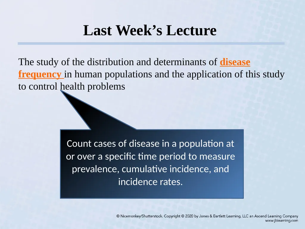
Last Week’s Lecture The study of the distribution and determinants of disease frequency in human populations and the application of this study to control health problems<br>
04
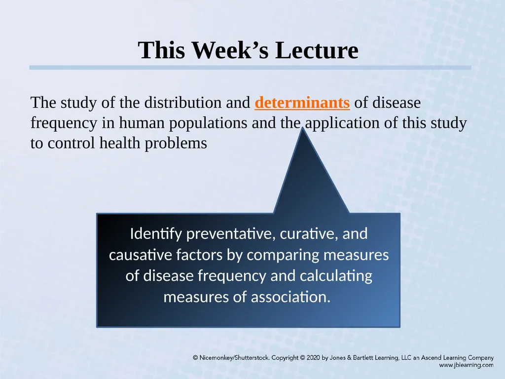
This Week’s Lecture The study of the distribution and determinants of disease frequency in human populations and the application of this study to control health problems Identify preventative, curative, and causative factors by comparing measures of disease frequency and calculating measures of association.<br>
05
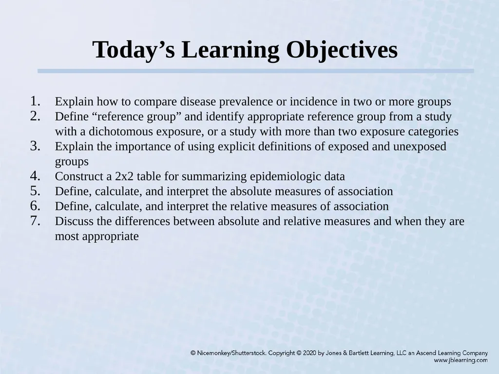
Today’s Learning Objectives Explain how to compare disease prevalence or incidence in two or more groups
Define “reference group” and identify appropriate reference group from a study with a dichotomous exposure, or a study with more than two exposure categories
Explain the importance of using explicit definitions of exposed and unexposed groups
Construct a 2x2 table for summarizing epidemiologic data
Define, calculate, and interpret the absolute measures of association
Define, calculate, and interpret the relative measures of association
Discuss the differences between absolute and relative measures and when they are most appropriate<br>
Define “reference group” and identify appropriate reference group from a study with a dichotomous exposure, or a study with more than two exposure categories
Explain the importance of using explicit definitions of exposed and unexposed groups
Construct a 2x2 table for summarizing epidemiologic data
Define, calculate, and interpret the absolute measures of association
Define, calculate, and interpret the relative measures of association
Discuss the differences between absolute and relative measures and when they are most appropriate<br>
06
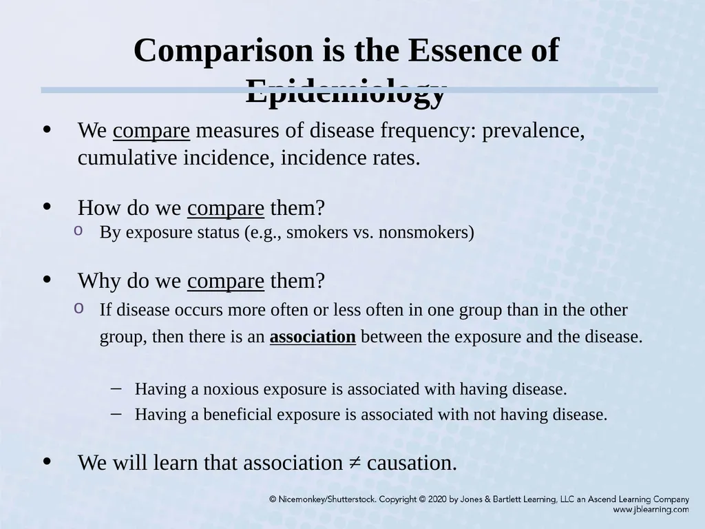
Comparison is the Essence of Epidemiology We compare measures of disease frequency: prevalence, cumulative incidence, incidence rates.
How do we compare them?
By exposure status (e.g., smokers vs. nonsmokers)
Why do we compare them?
If disease occurs more often or less often in one group than in the other group, then there is an association between the exposure and the disease.
Having a noxious exposure is associated with having disease.
Having a beneficial exposure is associated with not having disease.
We will learn that association ≠ causation.<br>
How do we compare them?
By exposure status (e.g., smokers vs. nonsmokers)
Why do we compare them?
If disease occurs more often or less often in one group than in the other group, then there is an association between the exposure and the disease.
Having a noxious exposure is associated with having disease.
Having a beneficial exposure is associated with not having disease.
We will learn that association ≠ causation.<br>
07
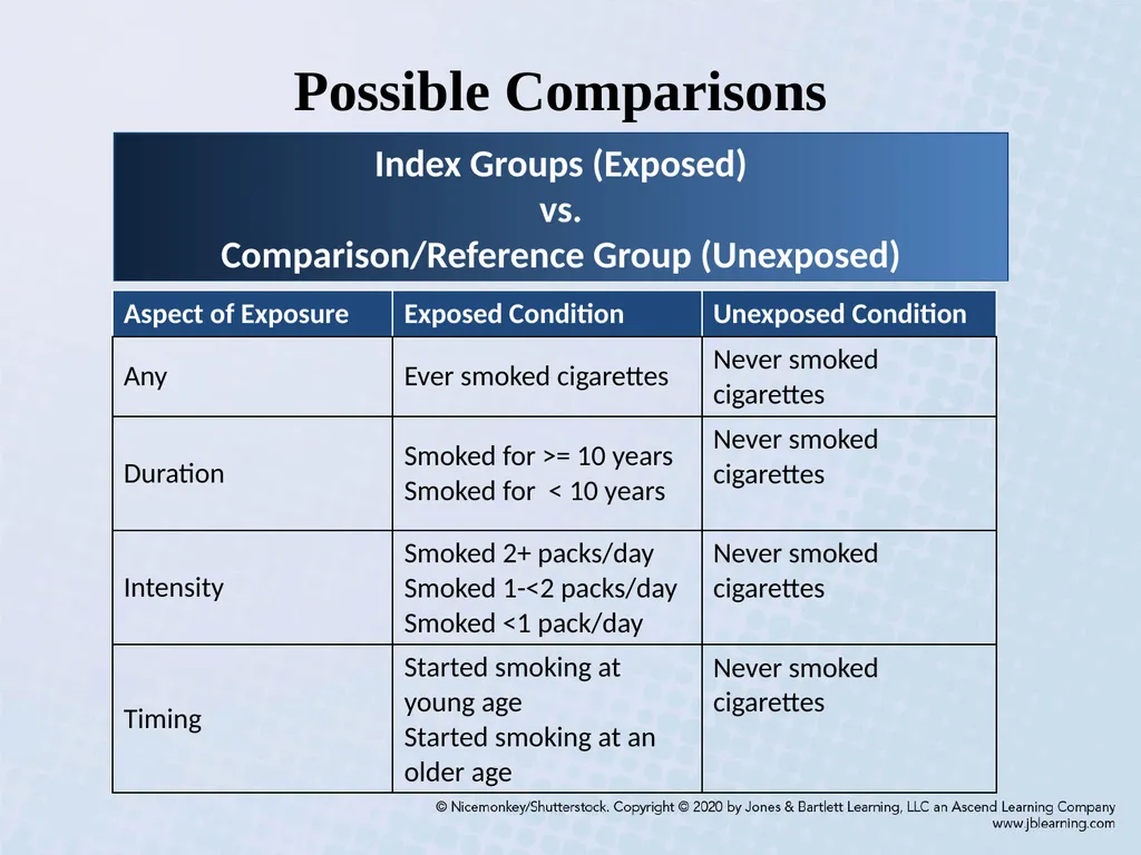
Possible Comparisons Index Groups (Exposed)
vs.
Comparison/Reference Group (Unexposed)<br>
vs.
Comparison/Reference Group (Unexposed)<br>
08
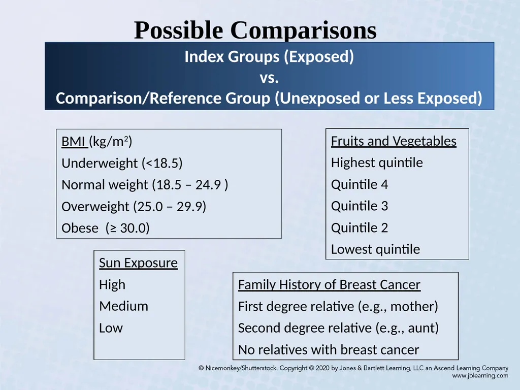
Possible Comparisons Index Groups (Exposed)
vs.
Comparison/Reference Group (Unexposed or Less Exposed) Sun Exposure
High
Medium
Low Fruits and Vegetables
Highest quintile
Quintile 4
Quintile 3
Quintile 2
Lowest quintile BMI (kg/m2)
Underweight (<18.5)
Normal weight (18.5 – 24.9 )
Overweight (25.0 – 29.9)
Obese (≥ 30.0) Family History of Breast Cancer
First degree relative (e.g., mother)
Second degree relative (e.g., aunt)
No relatives with breast cancer<br>
vs.
Comparison/Reference Group (Unexposed or Less Exposed) Sun Exposure
High
Medium
Low Fruits and Vegetables
Highest quintile
Quintile 4
Quintile 3
Quintile 2
Lowest quintile BMI (kg/m2)
Underweight (<18.5)
Normal weight (18.5 – 24.9 )
Overweight (25.0 – 29.9)
Obese (≥ 30.0) Family History of Breast Cancer
First degree relative (e.g., mother)
Second degree relative (e.g., aunt)
No relatives with breast cancer<br>
09
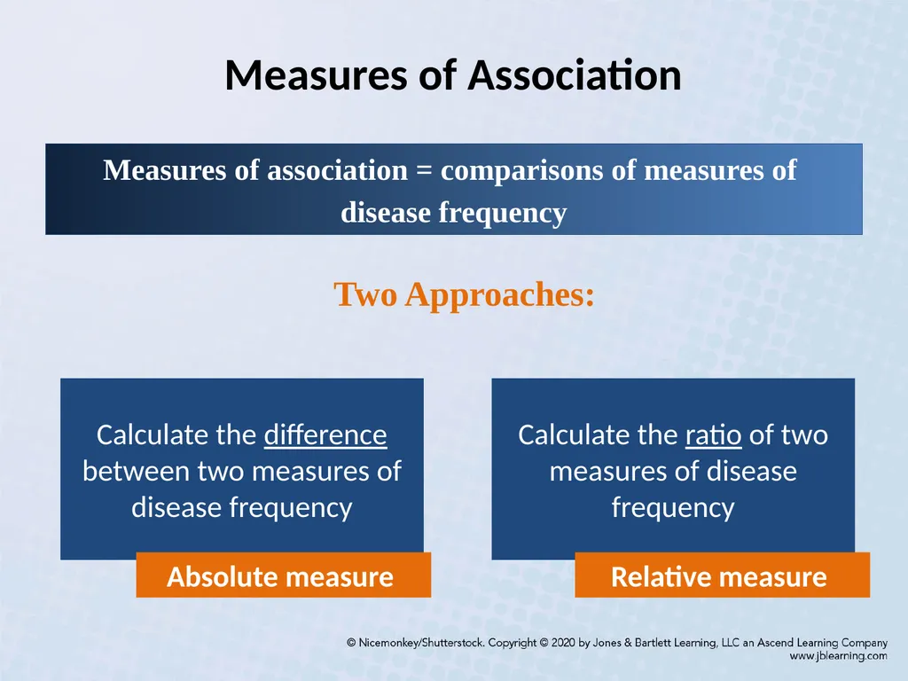
Measures of Association Measures of association = comparisons of measures of
disease frequency Two Approaches: Calculate the difference between two measures of disease frequency Calculate the ratio of two measures of disease frequency Absolute measure Relative measure<br>
disease frequency Two Approaches: Calculate the difference between two measures of disease frequency Calculate the ratio of two measures of disease frequency Absolute measure Relative measure<br>
10
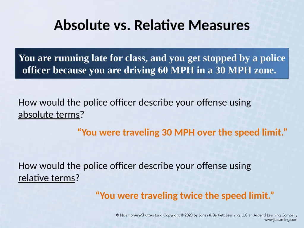
Absolute vs. Relative Measures You are running late for class, and you get stopped by a police officer because you are driving 60 MPH in a 30 MPH zone. “You were traveling 30 MPH over the speed limit.” How would the police officer describe your offense using absolute terms? “You were traveling twice the speed limit.” How would the police officer describe your offense using relative terms?<br>
11
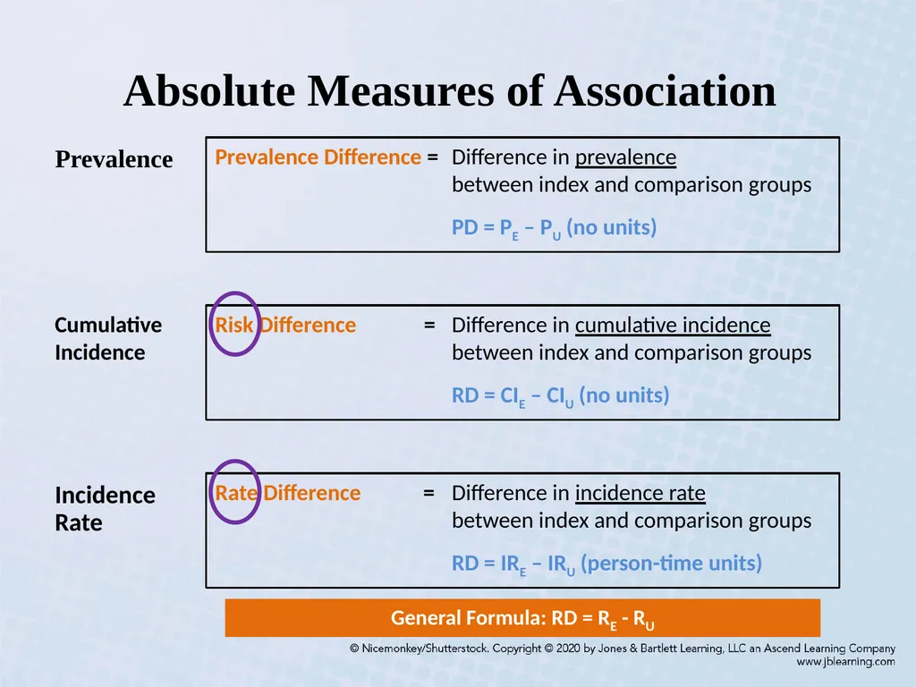
Absolute Measures of Association Prevalence Cumulative Incidence Incidence Rate General Formula: RD = RE - RU<br>
12
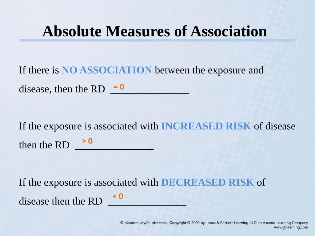
Absolute Measures of Association If there is NO ASSOCIATION between the exposure and disease, then the RD _______________
If the exposure is associated with INCREASED RISK of disease then the RD _______________
If the exposure is associated with DECREASED RISK of disease then the RD _______________ = 0 > 0 < 0<br>
If the exposure is associated with INCREASED RISK of disease then the RD _______________
If the exposure is associated with DECREASED RISK of disease then the RD _______________ = 0 > 0 < 0<br>
13
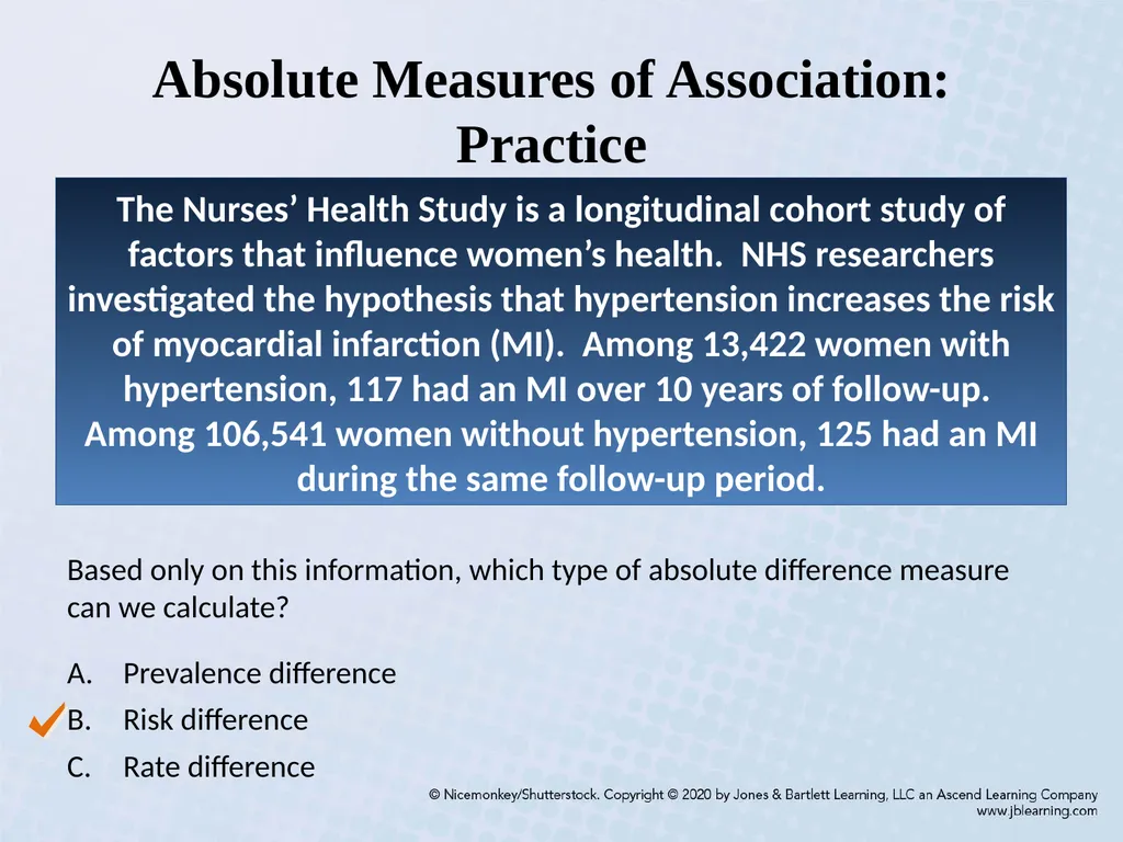
Absolute Measures of Association: Practice The Nurses’ Health Study is a longitudinal cohort study of factors that influence women’s health. NHS researchers investigated the hypothesis that hypertension increases the risk of myocardial infarction (MI). Among 13,422 women with hypertension, 117 had an MI over 10 years of follow-up. Among 106,541 women without hypertension, 125 had an MI during the same follow-up period. Based only on this information, which type of absolute difference measure can we calculate?
Prevalence difference
Risk difference
Rate difference<br>
Prevalence difference
Risk difference
Rate difference<br>
14
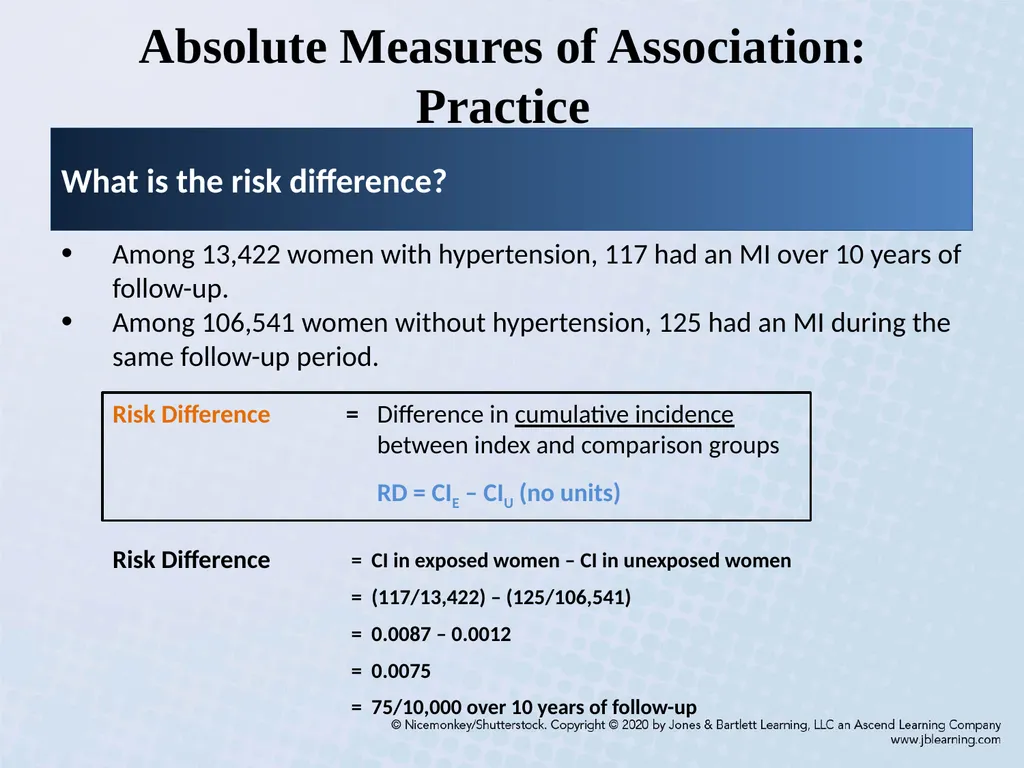
Absolute Measures of Association: Practice What is the risk difference? Among 13,422 women with hypertension, 117 had an MI over 10 years of follow-up.
Among 106,541 women without hypertension, 125 had an MI during the same follow-up period.<br>
Among 106,541 women without hypertension, 125 had an MI during the same follow-up period.<br>
15
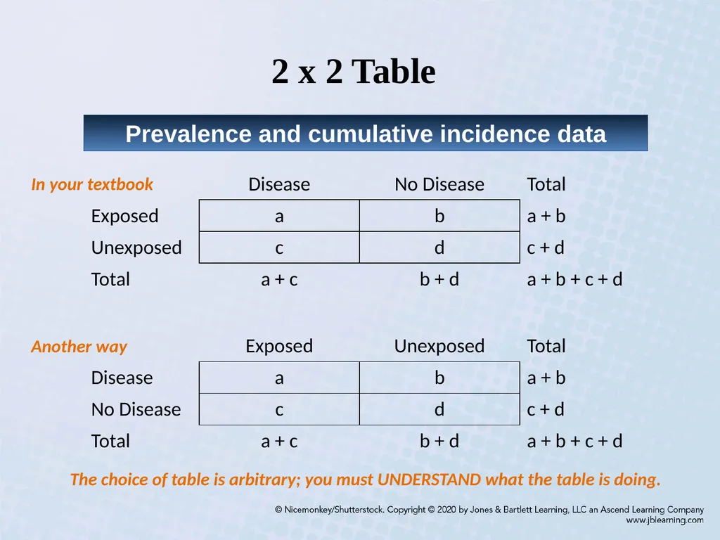
2 x 2 Table Prevalence and cumulative incidence data In your textbook Another way The choice of table is arbitrary; you must UNDERSTAND what the table is doing.<br>
16
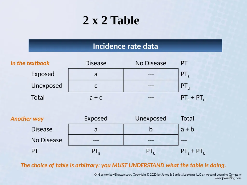
2 x 2 Table Incidence rate data In the textbook Another way The choice of table is arbitrary; you MUST UNDERSTAND what the table is doing. 16<br>
17
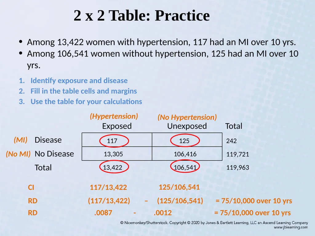
2 x 2 Table: Practice Among 13,422 women with hypertension, 117 had an MI over 10 yrs.
Among 106,541 women without hypertension, 125 had an MI over 10 yrs. Identify exposure and disease Fill in the table cells and margins Use the table for your calculations (Hypertension) (No Hypertension) (MI) (No MI) 117 13,305 13,422 125 106,416 106,541 242 119,721 119,963 RD (117/13,422) – (125/106,541) = 75/10,000 over 10 yrs RD .0087 - .0012 = 75/10,000 over 10 yrs<br>
Among 106,541 women without hypertension, 125 had an MI over 10 yrs. Identify exposure and disease Fill in the table cells and margins Use the table for your calculations (Hypertension) (No Hypertension) (MI) (No MI) 117 13,305 13,422 125 106,416 106,541 242 119,721 119,963 RD (117/13,422) – (125/106,541) = 75/10,000 over 10 yrs RD .0087 - .0012 = 75/10,000 over 10 yrs<br>
18
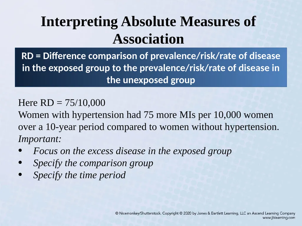
Interpreting Absolute Measures of Association Here RD = 75/10,000
Women with hypertension had 75 more MIs per 10,000 women over a 10-year period compared to women without hypertension.
Important:
Focus on the excess disease in the exposed group
Specify the comparison group
Specify the time period RD = Difference comparison of prevalence/risk/rate of disease in the exposed group to the prevalence/risk/rate of disease in the unexposed group<br>
Women with hypertension had 75 more MIs per 10,000 women over a 10-year period compared to women without hypertension.
Important:
Focus on the excess disease in the exposed group
Specify the comparison group
Specify the time period RD = Difference comparison of prevalence/risk/rate of disease in the exposed group to the prevalence/risk/rate of disease in the unexposed group<br>
19
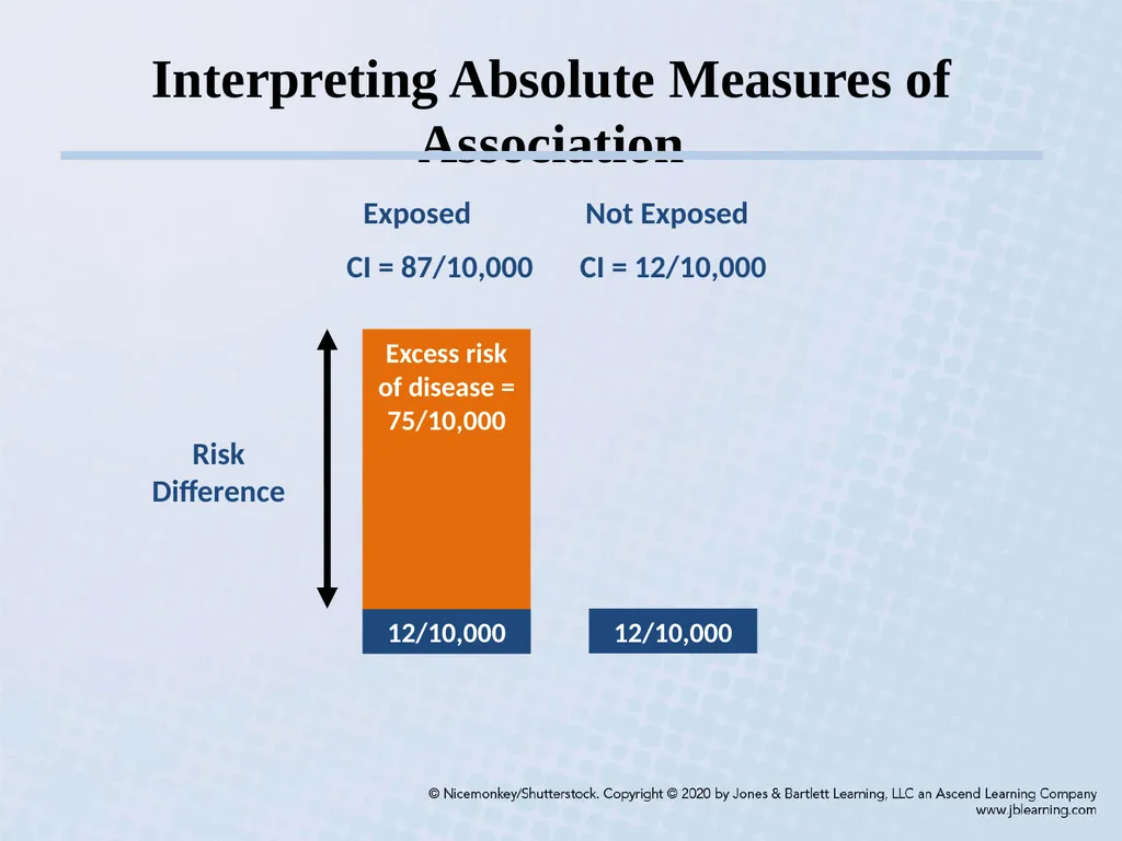
Interpreting Absolute Measures of Association Risk Difference<br>
20
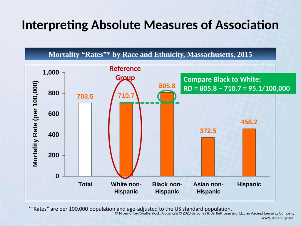
Mortality “Rates”* by Race and Ethnicity, Massachusetts, 2015 *“Rates” are per 100,000 population and age-adjusted to the US standard population. Interpreting Absolute Measures of Association Compare Black to White:
RD = 805.8 – 710.7 = 95.1/100,000<br>
RD = 805.8 – 710.7 = 95.1/100,000<br>
21
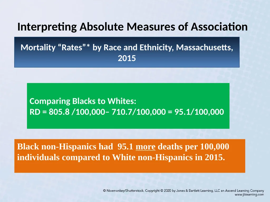
Interpreting Absolute Measures of Association Black non-Hispanics had 95.1 more deaths per 100,000 individuals compared to White non-Hispanics in 2015. Comparing Blacks to Whites:
RD = 805.8 /100,000– 710.7/100,000 = 95.1/100,000 Mortality “Rates”* by Race and Ethnicity, Massachusetts, 2015<br>
RD = 805.8 /100,000– 710.7/100,000 = 95.1/100,000 Mortality “Rates”* by Race and Ethnicity, Massachusetts, 2015<br>
22
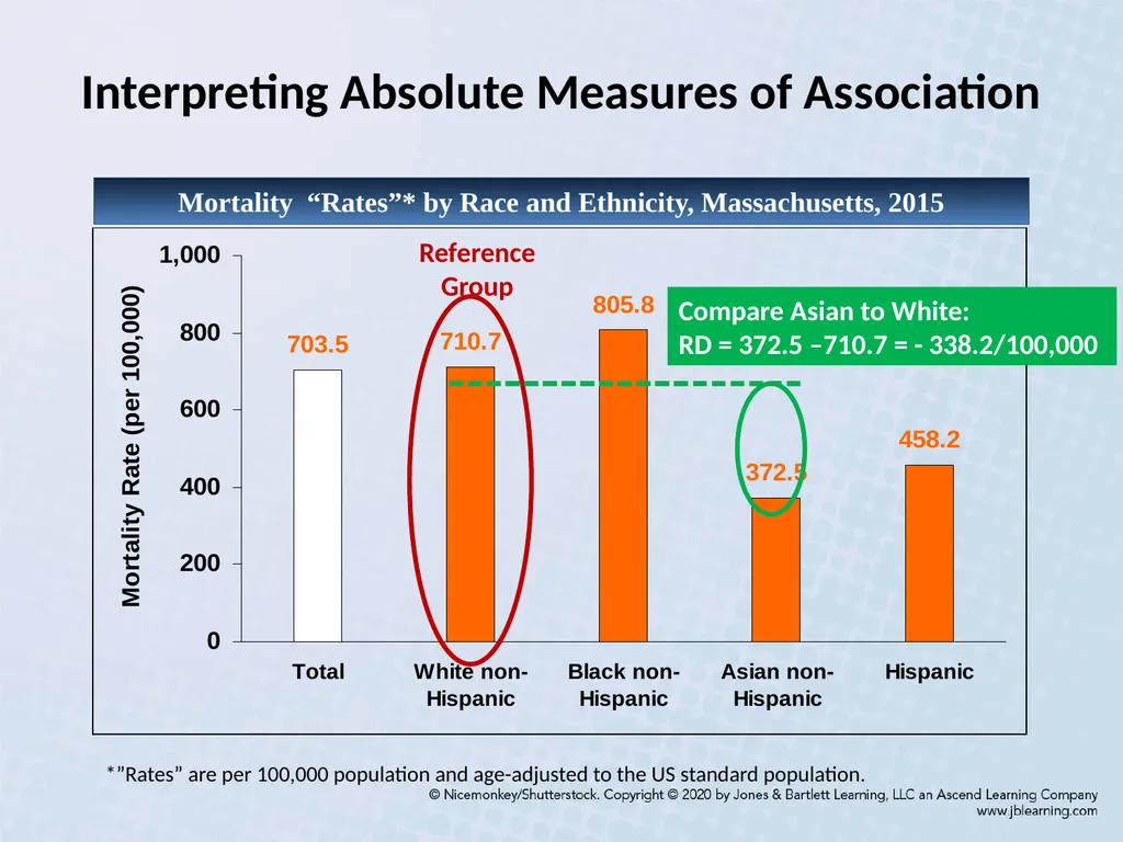
Mortality “Rates”* by Race and Ethnicity, Massachusetts, 2015 *”Rates” are per 100,000 population and age-adjusted to the US standard population. Interpreting Absolute Measures of Association Compare Asian to White:
RD = 372.5 –710.7 = - 338.2/100,000<br>
RD = 372.5 –710.7 = - 338.2/100,000<br>
23
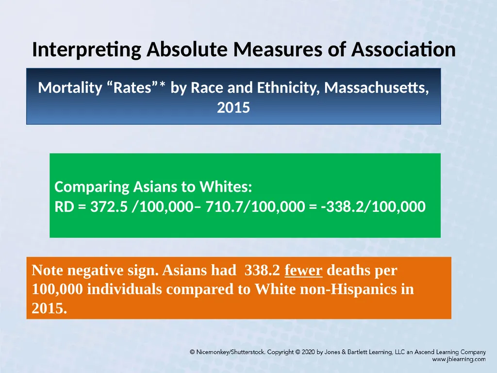
Interpreting Absolute Measures of Association Note negative sign. Asians had 338.2 fewer deaths per 100,000 individuals compared to White non-Hispanics in 2015. Comparing Asians to Whites:
RD = 372.5 /100,000– 710.7/100,000 = -338.2/100,000 Mortality “Rates”* by Race and Ethnicity, Massachusetts, 2015<br>
RD = 372.5 /100,000– 710.7/100,000 = -338.2/100,000 Mortality “Rates”* by Race and Ethnicity, Massachusetts, 2015<br>
24
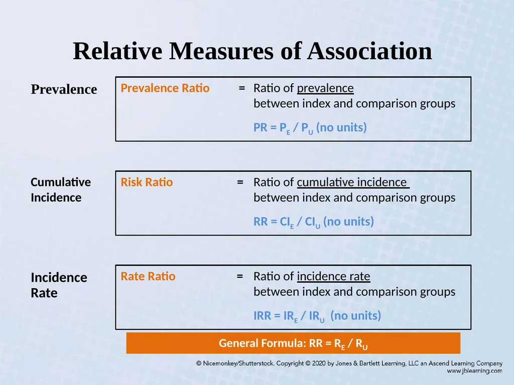
Relative Measures of Association Prevalence Cumulative Incidence Incidence Rate General Formula: RR = RE / RU<br>
25
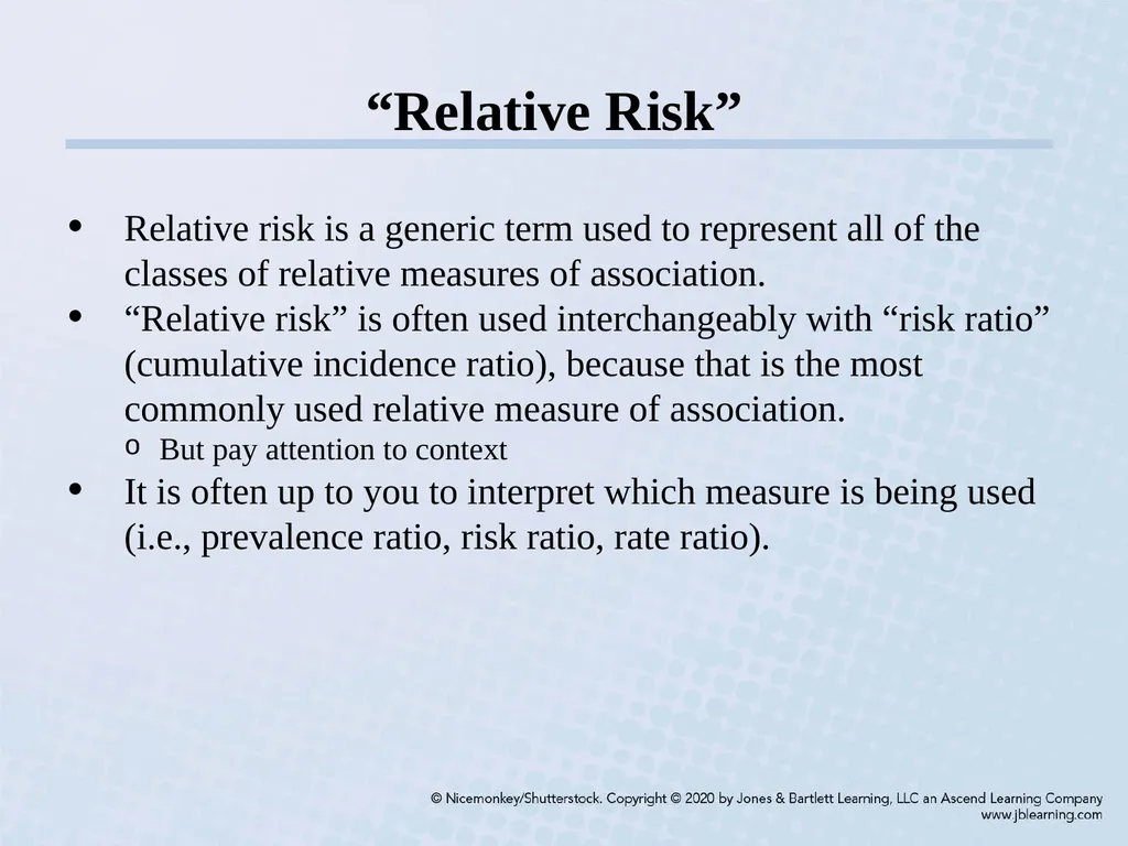
“Relative Risk” Relative risk is a generic term used to represent all of the classes of relative measures of association.
“Relative risk” is often used interchangeably with “risk ratio” (cumulative incidence ratio), because that is the most commonly used relative measure of association.
But pay attention to context
It is often up to you to interpret which measure is being used (i.e., prevalence ratio, risk ratio, rate ratio).<br>
“Relative risk” is often used interchangeably with “risk ratio” (cumulative incidence ratio), because that is the most commonly used relative measure of association.
But pay attention to context
It is often up to you to interpret which measure is being used (i.e., prevalence ratio, risk ratio, rate ratio).<br>
26
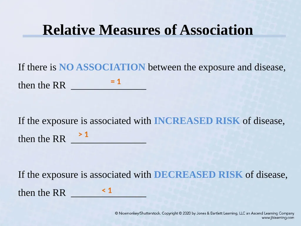
Relative Measures of Association If there is NO ASSOCIATION between the exposure and disease, then the RR _______________
If the exposure is associated with INCREASED RISK of disease, then the RR _______________
If the exposure is associated with DECREASED RISK of disease, then the RR _______________ = 1 > 1 < 1<br>
If the exposure is associated with INCREASED RISK of disease, then the RR _______________
If the exposure is associated with DECREASED RISK of disease, then the RR _______________ = 1 > 1 < 1<br>
27
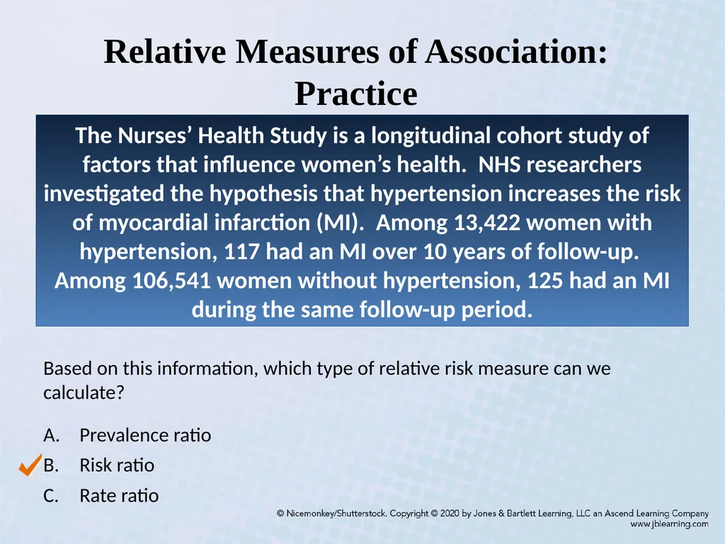
Relative Measures of Association: Practice The Nurses’ Health Study is a longitudinal cohort study of factors that influence women’s health. NHS researchers investigated the hypothesis that hypertension increases the risk of myocardial infarction (MI). Among 13,422 women with hypertension, 117 had an MI over 10 years of follow-up. Among 106,541 women without hypertension, 125 had an MI during the same follow-up period. Based on this information, which type of relative risk measure can we calculate?
Prevalence ratio
Risk ratio
Rate ratio<br>
Prevalence ratio
Risk ratio
Rate ratio<br>
28
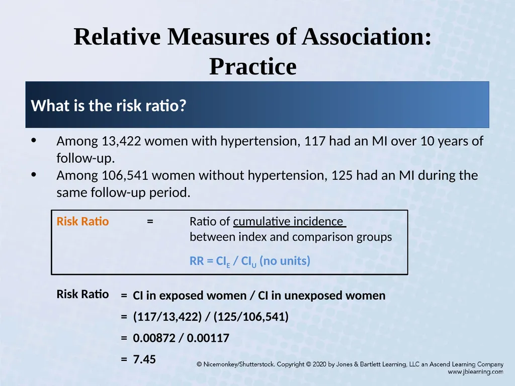
Relative Measures of Association: Practice What is the risk ratio? Among 13,422 women with hypertension, 117 had an MI over 10 years of follow-up.
Among 106,541 women without hypertension, 125 had an MI during the same follow-up period.<br>
Among 106,541 women without hypertension, 125 had an MI during the same follow-up period.<br>
29
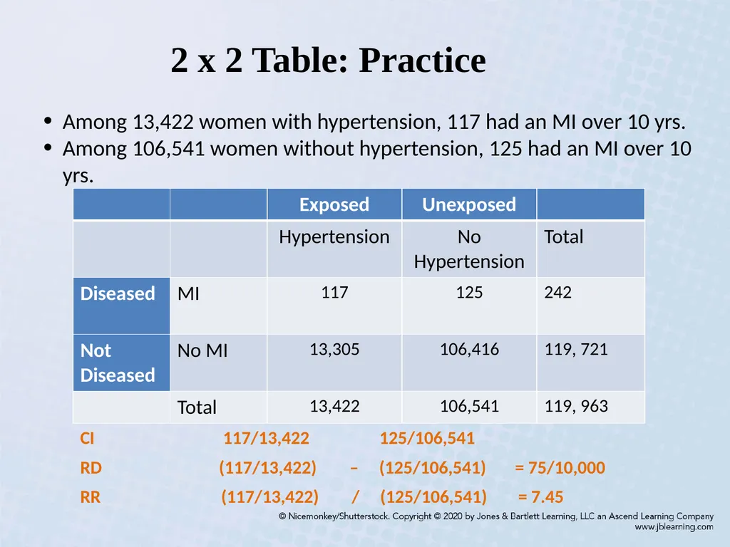
2 x 2 Table: Practice Among 13,422 women with hypertension, 117 had an MI over 10 yrs.
Among 106,541 women without hypertension, 125 had an MI over 10 yrs. CI 117/13,422 125/106,541 RR (117/13,422) / (125/106,541) = 7.45 RD (117/13,422) – (125/106,541) = 75/10,000<br>
Among 106,541 women without hypertension, 125 had an MI over 10 yrs. CI 117/13,422 125/106,541 RR (117/13,422) / (125/106,541) = 7.45 RD (117/13,422) – (125/106,541) = 75/10,000<br>
30
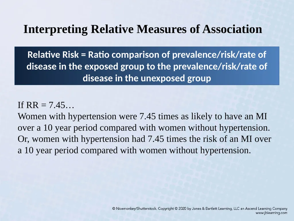
Interpreting Relative Measures of Association If RR = 7.45…
Women with hypertension were 7.45 times as likely to have an MI over a 10 year period compared with women without hypertension.
Or, women with hypertension had 7.45 times the risk of an MI over a 10 year period compared with women without hypertension. Relative Risk = Ratio comparison of prevalence/risk/rate of disease in the exposed group to the prevalence/risk/rate of disease in the unexposed group<br>
Women with hypertension were 7.45 times as likely to have an MI over a 10 year period compared with women without hypertension.
Or, women with hypertension had 7.45 times the risk of an MI over a 10 year period compared with women without hypertension. Relative Risk = Ratio comparison of prevalence/risk/rate of disease in the exposed group to the prevalence/risk/rate of disease in the unexposed group<br>
31
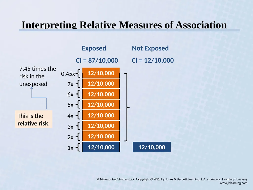
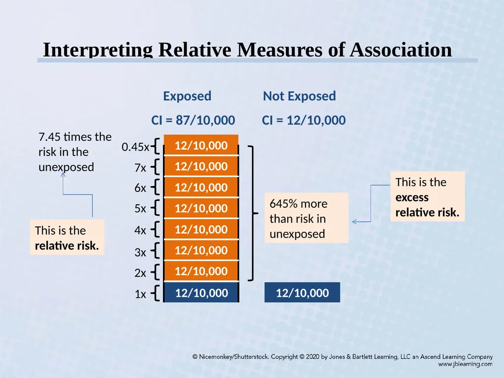
Interpreting Relative Measures of Association 7.45 times the risk in the unexposed This is the relative risk.<br>
32
Interpreting Relative Measures of Association 645% more than risk in unexposed 7.45 times the risk in the unexposed This is the excess relative risk. This is the relative risk.<br>
33
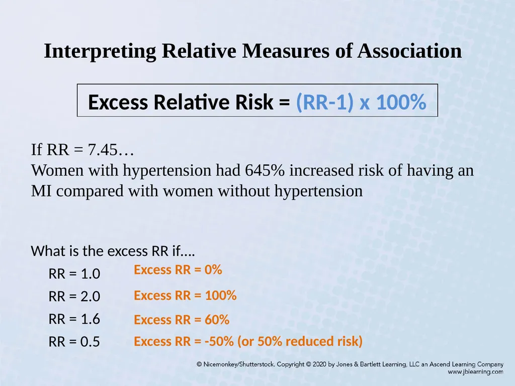
Interpreting Relative Measures of Association If RR = 7.45…
Women with hypertension had 645% increased risk of having an MI compared with women without hypertension Excess Relative Risk = (RR-1) x 100% What is the excess RR if….
RR = 1.0
RR = 2.0
RR = 1.6
RR = 0.5 Excess RR = 0% Excess RR = 100% Excess RR = 60% Excess RR = -50% (or 50% reduced risk)<br>
Women with hypertension had 645% increased risk of having an MI compared with women without hypertension Excess Relative Risk = (RR-1) x 100% What is the excess RR if….
RR = 1.0
RR = 2.0
RR = 1.6
RR = 0.5 Excess RR = 0% Excess RR = 100% Excess RR = 60% Excess RR = -50% (or 50% reduced risk)<br>
34
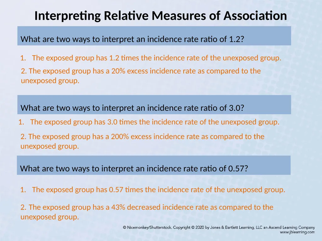
Interpreting Relative Measures of Association What are two ways to interpret an incidence rate ratio of 1.2? What are two ways to interpret an incidence rate ratio of 3.0? What are two ways to interpret an incidence rate ratio of 0.57? The exposed group has 1.2 times the incidence rate of the unexposed group. The exposed group has 3.0 times the incidence rate of the unexposed group. The exposed group has 0.57 times the incidence rate of the unexposed group. 2. The exposed group has a 20% excess incidence rate as compared to the unexposed group. 2. The exposed group has a 200% excess incidence rate as compared to the unexposed group. 2. The exposed group has a 43% decreased incidence rate as compared to the unexposed group.<br>
35
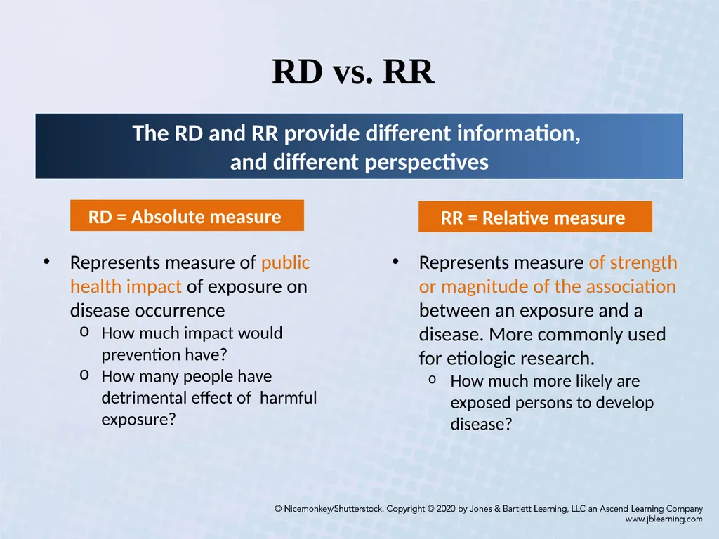
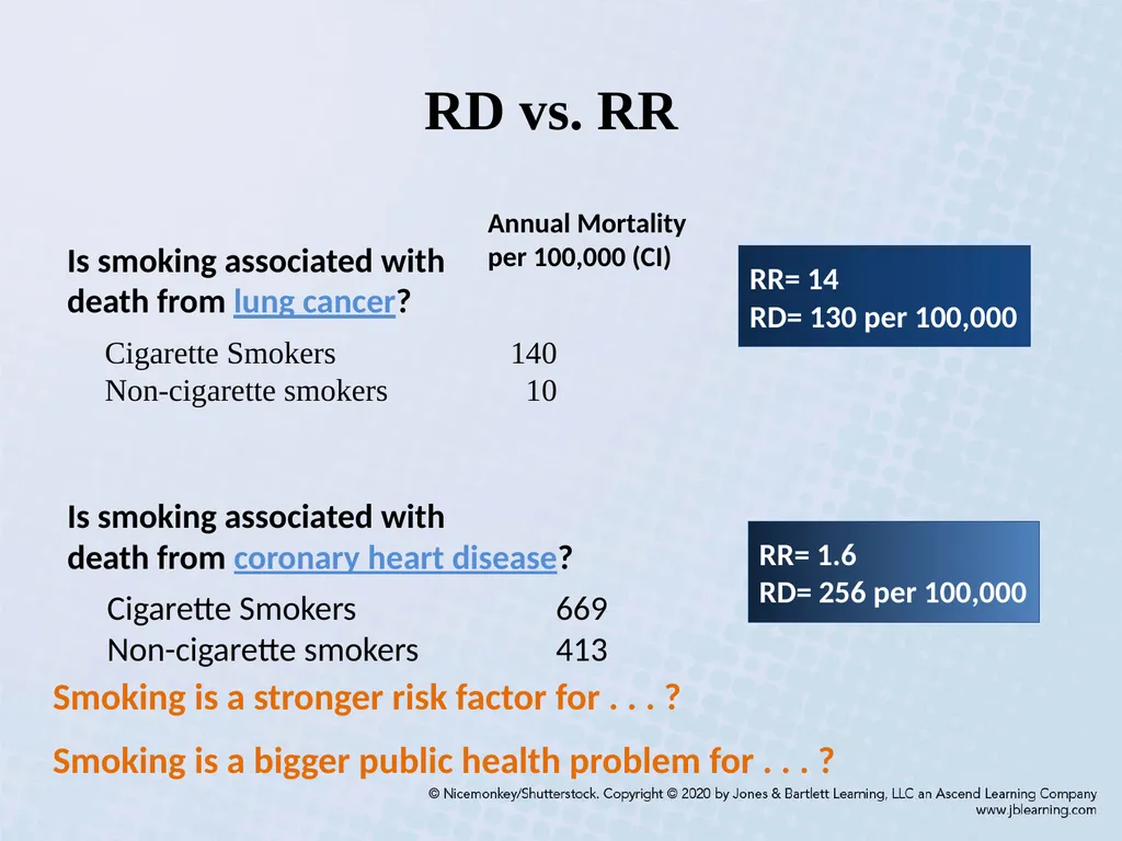
RD vs. RR The RD and RR provide different information,
and different perspectives Represents measure of strength or magnitude of the association between an exposure and a disease. More commonly used for etiologic research.
How much more likely are exposed persons to develop disease? Represents measure of public health impact of exposure on disease occurrence
How much impact would prevention have?
How many people have detrimental effect of harmful exposure? RD = Absolute measure RR = Relative measure<br>
and different perspectives Represents measure of strength or magnitude of the association between an exposure and a disease. More commonly used for etiologic research.
How much more likely are exposed persons to develop disease? Represents measure of public health impact of exposure on disease occurrence
How much impact would prevention have?
How many people have detrimental effect of harmful exposure? RD = Absolute measure RR = Relative measure<br>
36
Recall slide from first class:
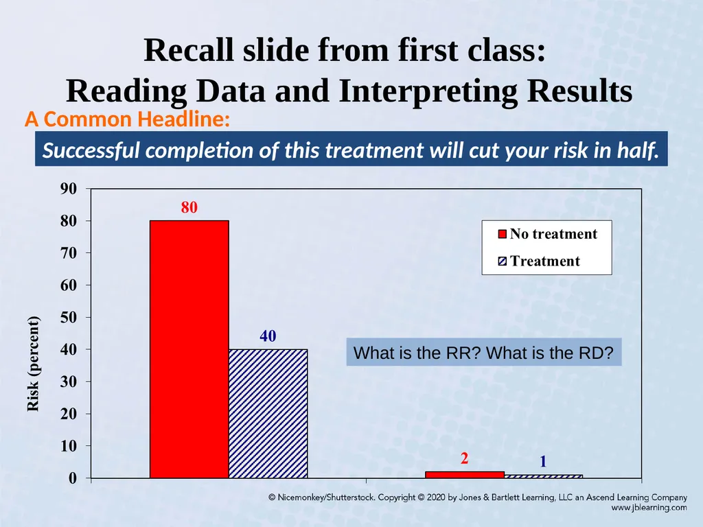
Reading Data and Interpreting Results Successful completion of this treatment will cut your risk in half. A Common Headline: What is the RR? What is the RD?<br>
37
RD vs. RR Cigarette Smokers 140
Non-cigarette smokers 10 Cigarette Smokers 669
Non-cigarette smokers 413 Annual Mortality
per 100,000 (CI) Is smoking associated with
death from lung cancer? Is smoking associated with
death from coronary heart disease? Smoking is a stronger risk factor for . . . ?
Smoking is a bigger public health problem for . . . ? RR= 1.6
RD= 256 per 100,000 RR= 14
RD= 130 per 100,000<br>
Non-cigarette smokers 10 Cigarette Smokers 669
Non-cigarette smokers 413 Annual Mortality
per 100,000 (CI) Is smoking associated with
death from lung cancer? Is smoking associated with
death from coronary heart disease? Smoking is a stronger risk factor for . . . ?
Smoking is a bigger public health problem for . . . ? RR= 1.6
RD= 256 per 100,000 RR= 14
RD= 130 per 100,000<br>
38
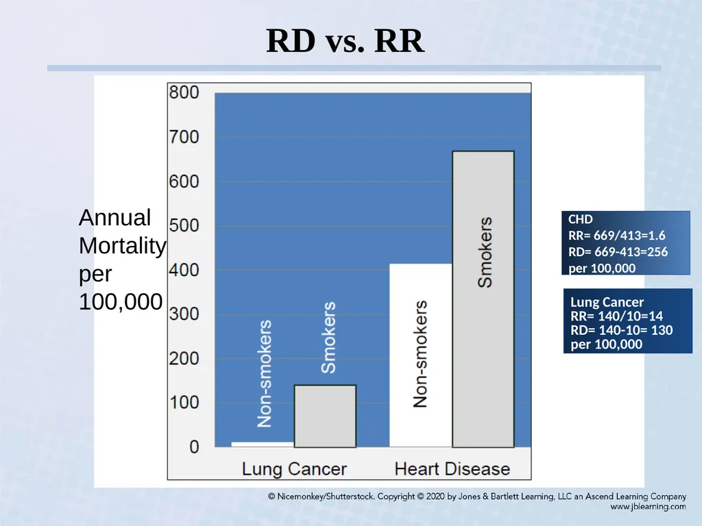
RD vs. RR Annual
Mortality
per
100,000 CHD
RR= 669/413=1.6
RD= 669-413=256 per 100,000 Lung Cancer
RR= 140/10=14
RD= 140-10= 130 per 100,000<br>
Mortality
per
100,000 CHD
RR= 669/413=1.6
RD= 669-413=256 per 100,000 Lung Cancer
RR= 140/10=14
RD= 140-10= 130 per 100,000<br>
39
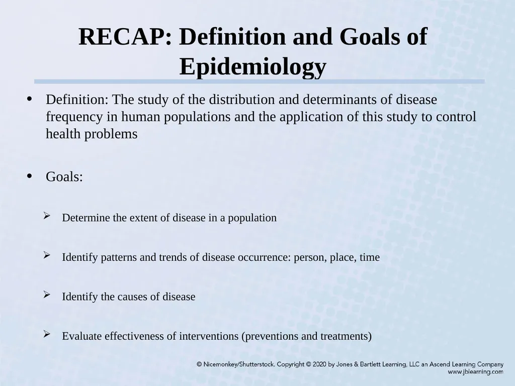
RECAP: Definition and Goals of Epidemiology Definition: The study of the distribution and determinants of disease frequency in human populations and the application of this study to control health problems
Goals:
Determine the extent of disease in a population
Identify patterns and trends of disease occurrence: person, place, time
Identify the causes of disease
Evaluate effectiveness of interventions (preventions and treatments)<br>
Goals:
Determine the extent of disease in a population
Identify patterns and trends of disease occurrence: person, place, time
Identify the causes of disease
Evaluate effectiveness of interventions (preventions and treatments)<br>
40
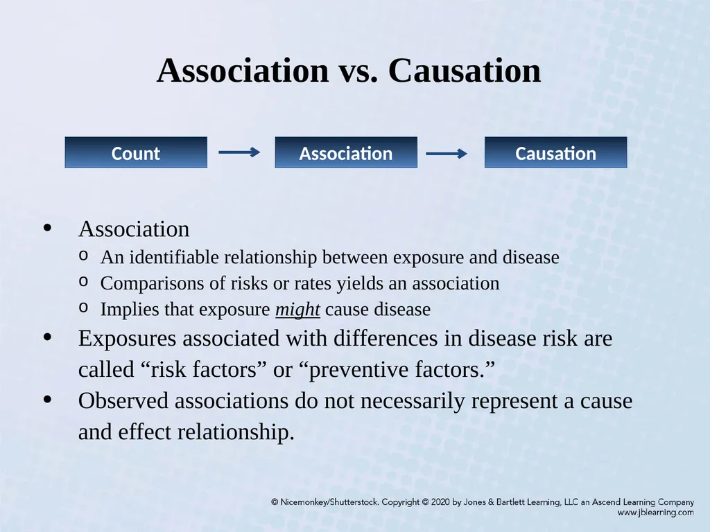
Association vs. Causation Association
An identifiable relationship between exposure and disease
Comparisons of risks or rates yields an association
Implies that exposure might cause disease
Exposures associated with differences in disease risk are called “risk factors” or “preventive factors.”
Observed associations do not necessarily represent a cause and effect relationship. Count Association Causation<br>
An identifiable relationship between exposure and disease
Comparisons of risks or rates yields an association
Implies that exposure might cause disease
Exposures associated with differences in disease risk are called “risk factors” or “preventive factors.”
Observed associations do not necessarily represent a cause and effect relationship. Count Association Causation<br>
41
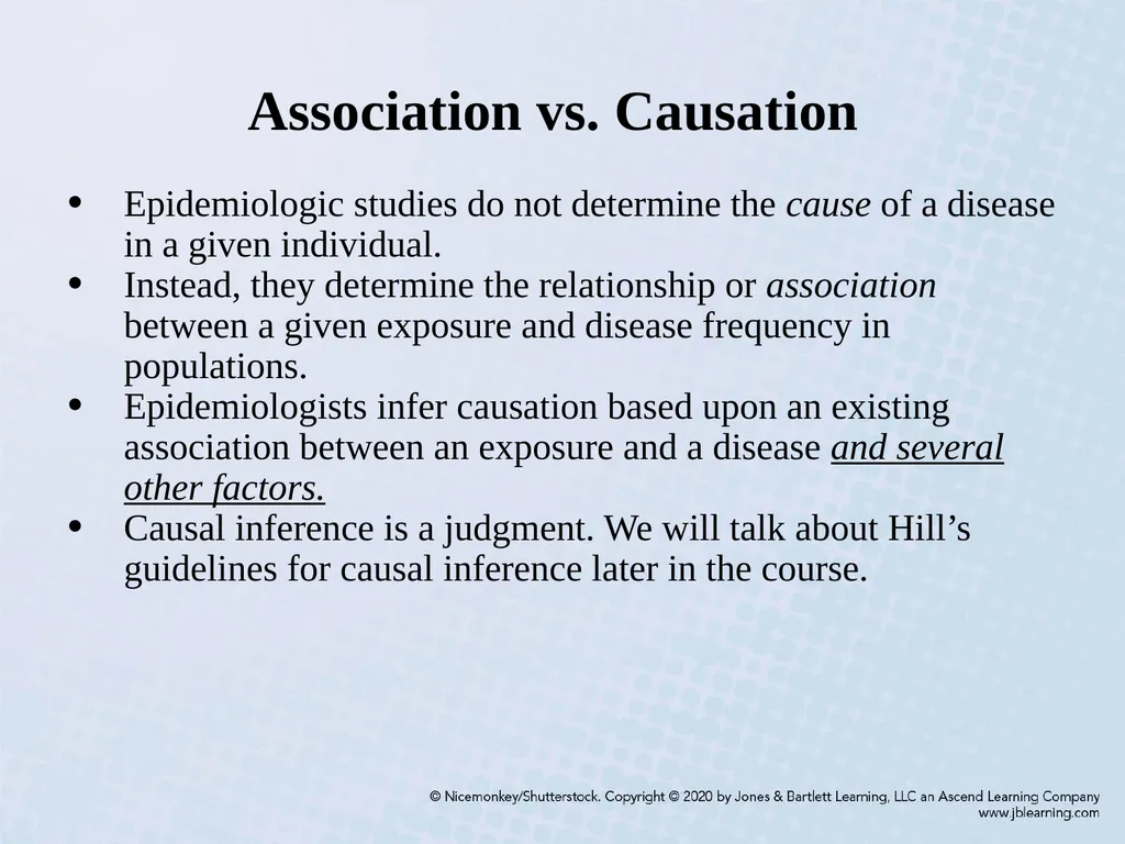
Association vs. Causation Epidemiologic studies do not determine the cause of a disease in a given individual.
Instead, they determine the relationship or association between a given exposure and disease frequency in populations.
Epidemiologists infer causation based upon an existing association between an exposure and a disease and several other factors.
Causal inference is a judgment. We will talk about Hill’s guidelines for causal inference later in the course.<br>
Instead, they determine the relationship or association between a given exposure and disease frequency in populations.
Epidemiologists infer causation based upon an existing association between an exposure and a disease and several other factors.
Causal inference is a judgment. We will talk about Hill’s guidelines for causal inference later in the course.<br>
42
Another Measure of Association:
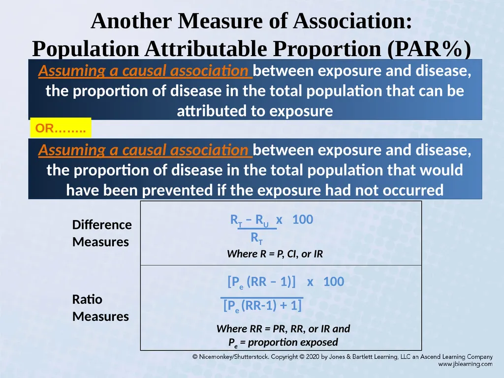
Population Attributable Proportion (PAR%) Assuming a causal association between exposure and disease, the proportion of disease in the total population that can be attributed to exposure Where R = P, CI, or IR Where RR = PR, RR, or IR and Pe = proportion exposed Assuming a causal association between exposure and disease, the proportion of disease in the total population that would have been prevented if the exposure had not occurred OR……..<br>
43
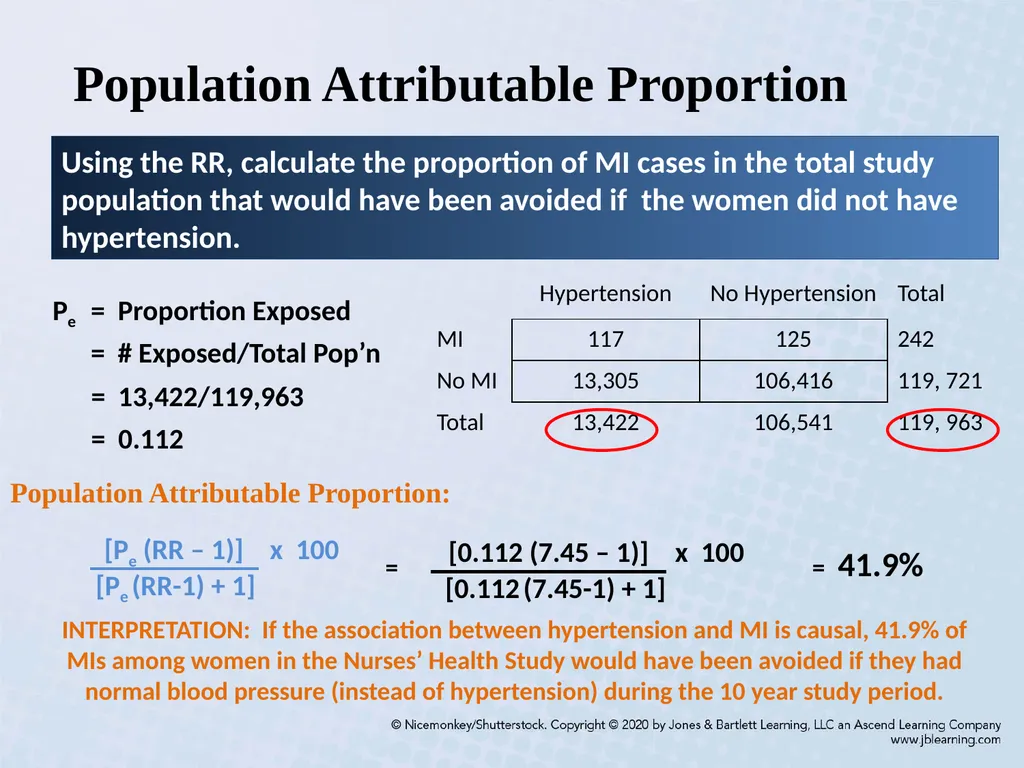
Population Attributable Proportion Population Attributable Proportion: Using the RR, calculate the proportion of MI cases in the total study population that would have been avoided if the women did not have hypertension. Pe = Proportion Exposed INTERPRETATION: If the association between hypertension and MI is causal, 41.9% of MIs among women in the Nurses’ Health Study would have been avoided if they had normal blood pressure (instead of hypertension) during the 10 year study period. = # Exposed/Total Pop’n = 13,422/119,963
= 0.112<br>
= 0.112<br>
44
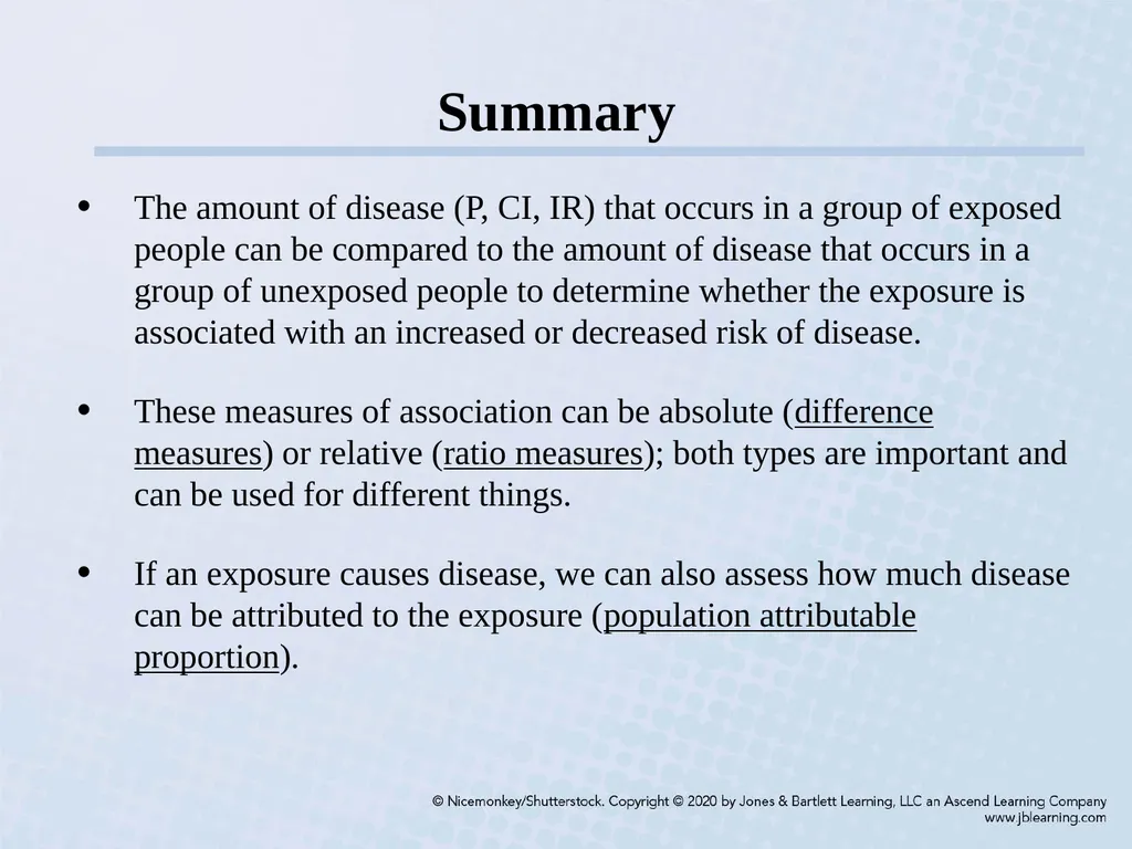
Summary The amount of disease (P, CI, IR) that occurs in a group of exposed people can be compared to the amount of disease that occurs in a group of unexposed people to determine whether the exposure is associated with an increased or decreased risk of disease.
These measures of association can be absolute (difference measures) or relative (ratio measures); both types are important and can be used for different things.
If an exposure causes disease, we can also assess how much disease can be attributed to the exposure (population attributable proportion).<br>
These measures of association can be absolute (difference measures) or relative (ratio measures); both types are important and can be used for different things.
If an exposure causes disease, we can also assess how much disease can be attributed to the exposure (population attributable proportion).<br>
45
PRACTICE<br>
46
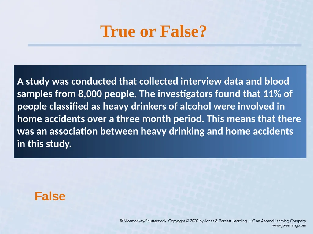
A study was conducted that collected interview data and blood samples from 8,000 people. The investigators found that 11% of people classified as heavy drinkers of alcohol were involved in home accidents over a three month period. This means that there was an association between heavy drinking and home accidents in this study. True or False? False<br>
47
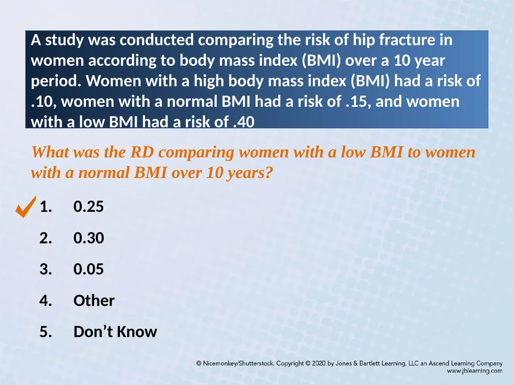
A study was conducted comparing the risk of hip fracture in women according to body mass index (BMI) over a 10 year period. Women with a high body mass index (BMI) had a risk of .10, women with a normal BMI had a risk of .15, and women with a low BMI had a risk of .40 What was the RD comparing women with a low BMI to women with a normal BMI over 10 years? 0.25
0.30
0.05
Other
Don’t Know<br>
0.30
0.05
Other
Don’t Know<br>
48
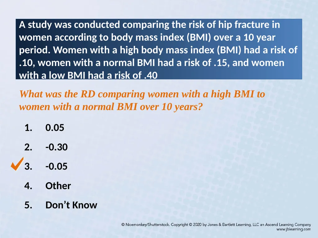
A study was conducted comparing the risk of hip fracture in women according to body mass index (BMI) over a 10 year period. Women with a high body mass index (BMI) had a risk of .10, women with a normal BMI had a risk of .15, and women with a low BMI had a risk of .40 What was the RD comparing women with a high BMI to women with a normal BMI over 10 years? 0.05
-0.30
-0.05
Other
Don’t Know<br>
-0.30
-0.05
Other
Don’t Know<br>
49
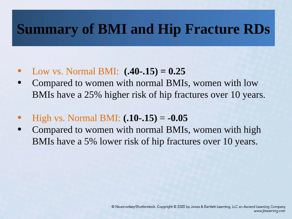
Summary of BMI and Hip Fracture RDs Low vs. Normal BMI: (.40-.15) = 0.25
Compared to women with normal BMIs, women with low BMIs have a 25% higher risk of hip fractures over 10 years.
High vs. Normal BMI: (.10-.15) = -0.05
Compared to women with normal BMIs, women with high BMIs have a 5% lower risk of hip fractures over 10 years.<br>
Compared to women with normal BMIs, women with low BMIs have a 25% higher risk of hip fractures over 10 years.
High vs. Normal BMI: (.10-.15) = -0.05
Compared to women with normal BMIs, women with high BMIs have a 5% lower risk of hip fractures over 10 years.<br>
50
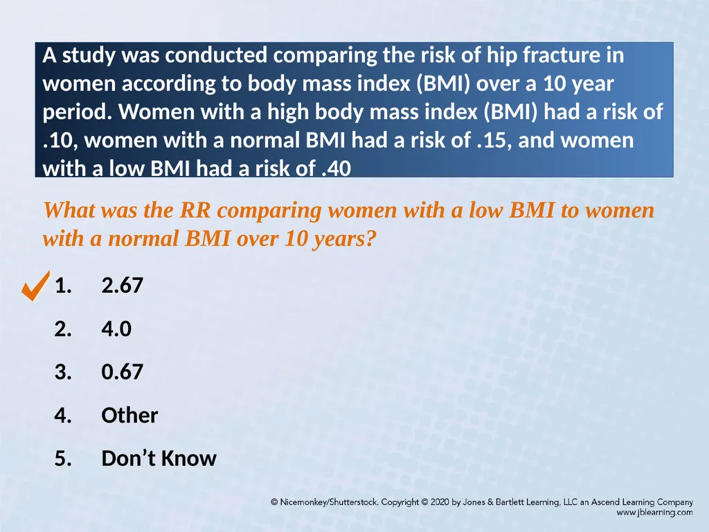
A study was conducted comparing the risk of hip fracture in women according to body mass index (BMI) over a 10 year period. Women with a high body mass index (BMI) had a risk of .10, women with a normal BMI had a risk of .15, and women with a low BMI had a risk of .40 What was the RR comparing women with a low BMI to women with a normal BMI over 10 years? 2.67
4.0
0.67
Other
Don’t Know<br>
4.0
0.67
Other
Don’t Know<br>
51
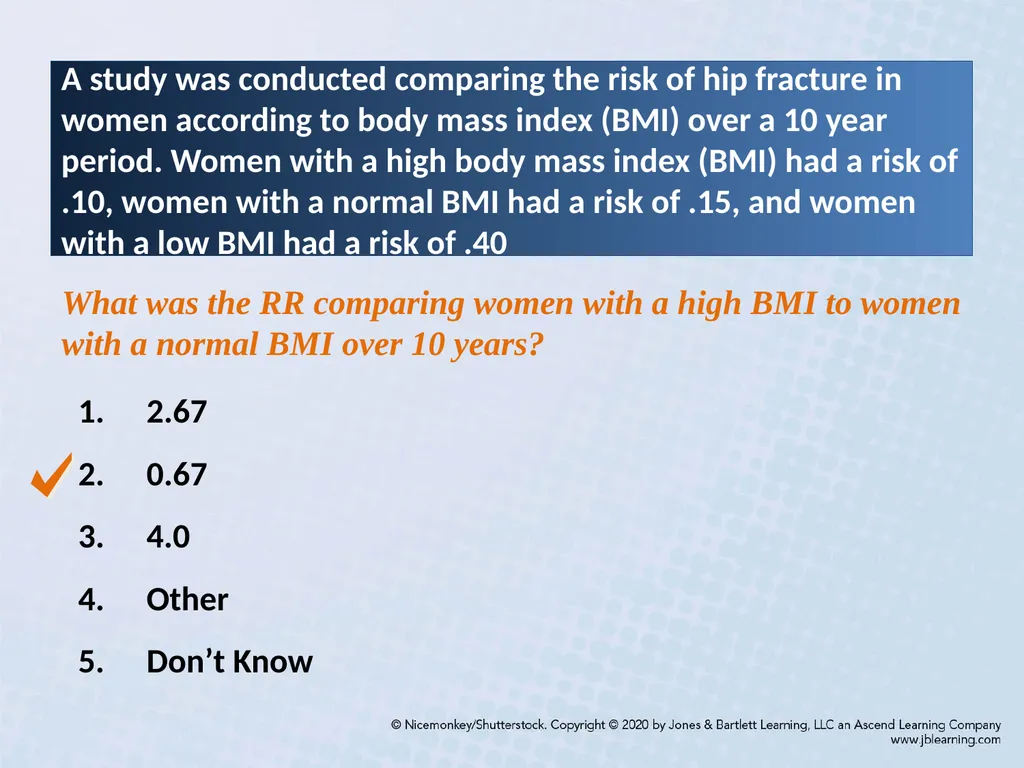
A study was conducted comparing the risk of hip fracture in women according to body mass index (BMI) over a 10 year period. Women with a high body mass index (BMI) had a risk of .10, women with a normal BMI had a risk of .15, and women with a low BMI had a risk of .40 What was the RR comparing women with a high BMI to women with a normal BMI over 10 years? 2.67
0.67
4.0
Other
Don’t Know<br>
0.67
4.0
Other
Don’t Know<br>
52
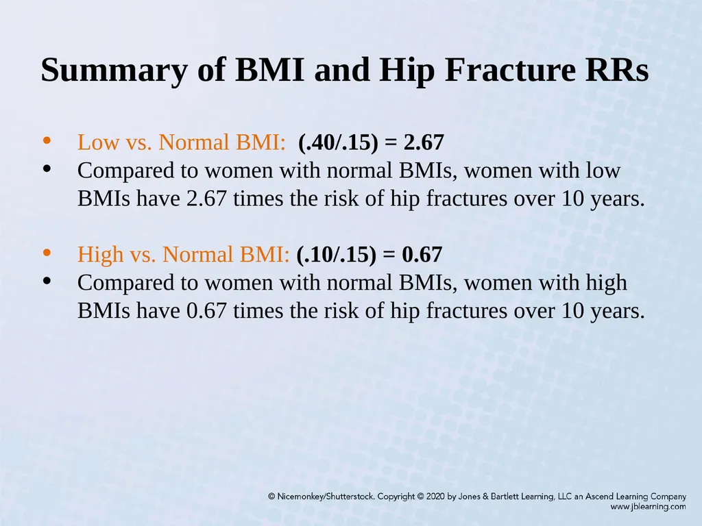
Summary of BMI and Hip Fracture RRs Low vs. Normal BMI: (.40/.15) = 2.67
Compared to women with normal BMIs, women with low BMIs have 2.67 times the risk of hip fractures over 10 years.
High vs. Normal BMI: (.10/.15) = 0.67
Compared to women with normal BMIs, women with high BMIs have 0.67 times the risk of hip fractures over 10 years.<br>
Compared to women with normal BMIs, women with low BMIs have 2.67 times the risk of hip fractures over 10 years.
High vs. Normal BMI: (.10/.15) = 0.67
Compared to women with normal BMIs, women with high BMIs have 0.67 times the risk of hip fractures over 10 years.<br>
53
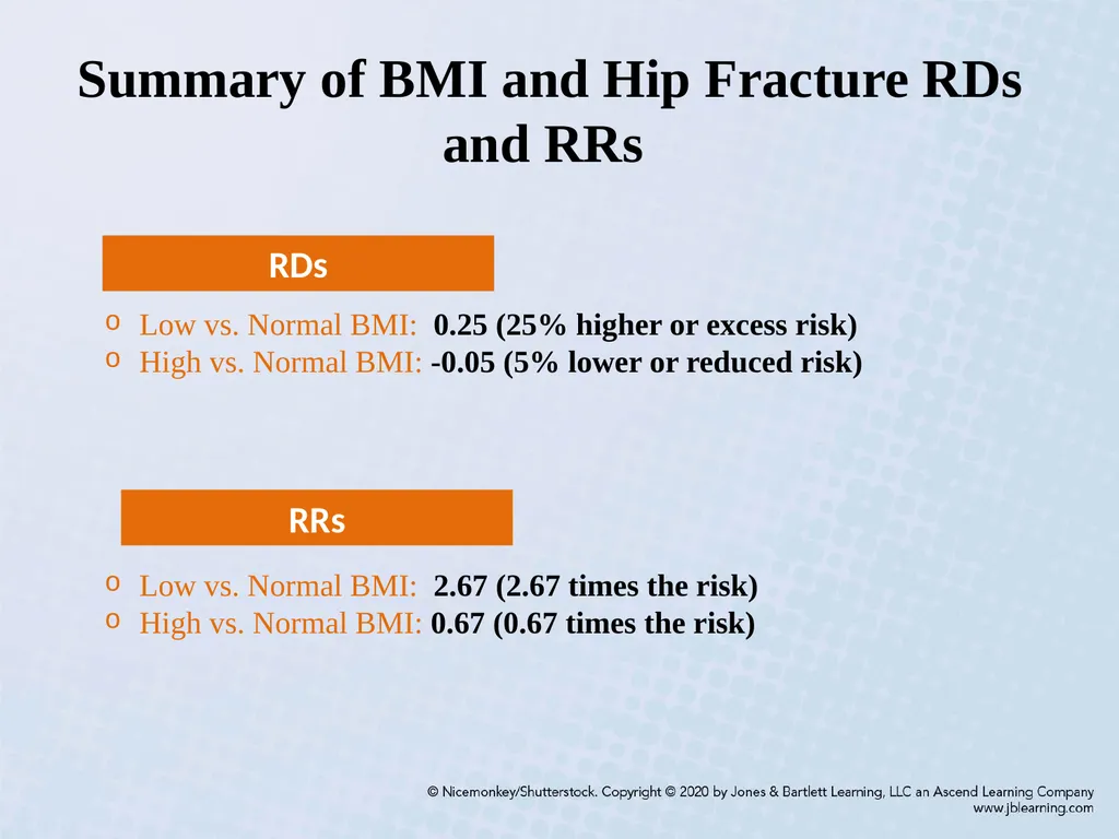
Summary of BMI and Hip Fracture RDs and RRs Low vs. Normal BMI: 0.25 (25% higher or excess risk)
High vs. Normal BMI: -0.05 (5% lower or reduced risk)
Low vs. Normal BMI: 2.67 (2.67 times the risk)
High vs. Normal BMI: 0.67 (0.67 times the risk) RDs RRs<br>
High vs. Normal BMI: -0.05 (5% lower or reduced risk)
Low vs. Normal BMI: 2.67 (2.67 times the risk)
High vs. Normal BMI: 0.67 (0.67 times the risk) RDs RRs<br>
54
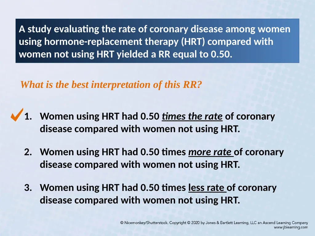
A study evaluating the rate of coronary disease among women using hormone-replacement therapy (HRT) compared with women not using HRT yielded a RR equal to 0.50. What is the best interpretation of this RR? Women using HRT had 0.50 times the rate of coronary disease compared with women not using HRT.
Women using HRT had 0.50 times more rate of coronary disease compared with women not using HRT.
Women using HRT had 0.50 times less rate of coronary disease compared with women not using HRT.<br>
Women using HRT had 0.50 times more rate of coronary disease compared with women not using HRT.
Women using HRT had 0.50 times less rate of coronary disease compared with women not using HRT.<br>
55
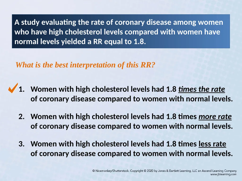
A study evaluating the rate of coronary disease among women who have high cholesterol levels compared with women have normal levels yielded a RR equal to 1.8. What is the best interpretation of this RR? Women with high cholesterol levels had 1.8 times the rate of coronary disease compared to women with normal levels.
Women with high cholesterol levels had 1.8 times more rate of coronary disease compared to women with normal levels.
Women with high cholesterol levels had 1.8 times less rate of coronary disease compared to women with normal levels.<br>
Women with high cholesterol levels had 1.8 times more rate of coronary disease compared to women with normal levels.
Women with high cholesterol levels had 1.8 times less rate of coronary disease compared to women with normal levels.<br>
56
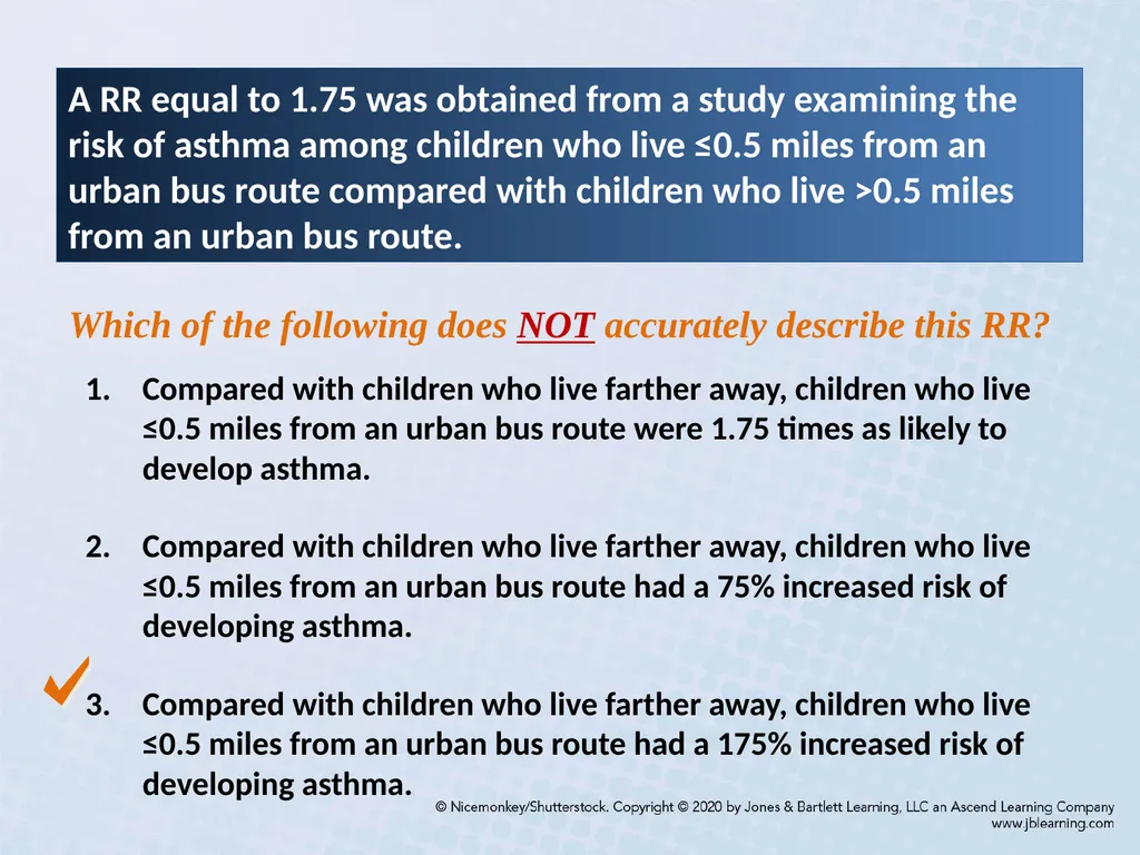
A RR equal to 1.75 was obtained from a study examining the risk of asthma among children who live ≤0.5 miles from an urban bus route compared with children who live ˃0.5 miles from an urban bus route. Which of the following does NOT accurately describe this RR? Compared with children who live farther away, children who live ≤0.5 miles from an urban bus route were 1.75 times as likely to develop asthma.
Compared with children who live farther away, children who live ≤0.5 miles from an urban bus route had a 75% increased risk of developing asthma.
Compared with children who live farther away, children who live ≤0.5 miles from an urban bus route had a 175% increased risk of developing asthma.<br>
Compared with children who live farther away, children who live ≤0.5 miles from an urban bus route had a 75% increased risk of developing asthma.
Compared with children who live farther away, children who live ≤0.5 miles from an urban bus route had a 175% increased risk of developing asthma.<br>
57
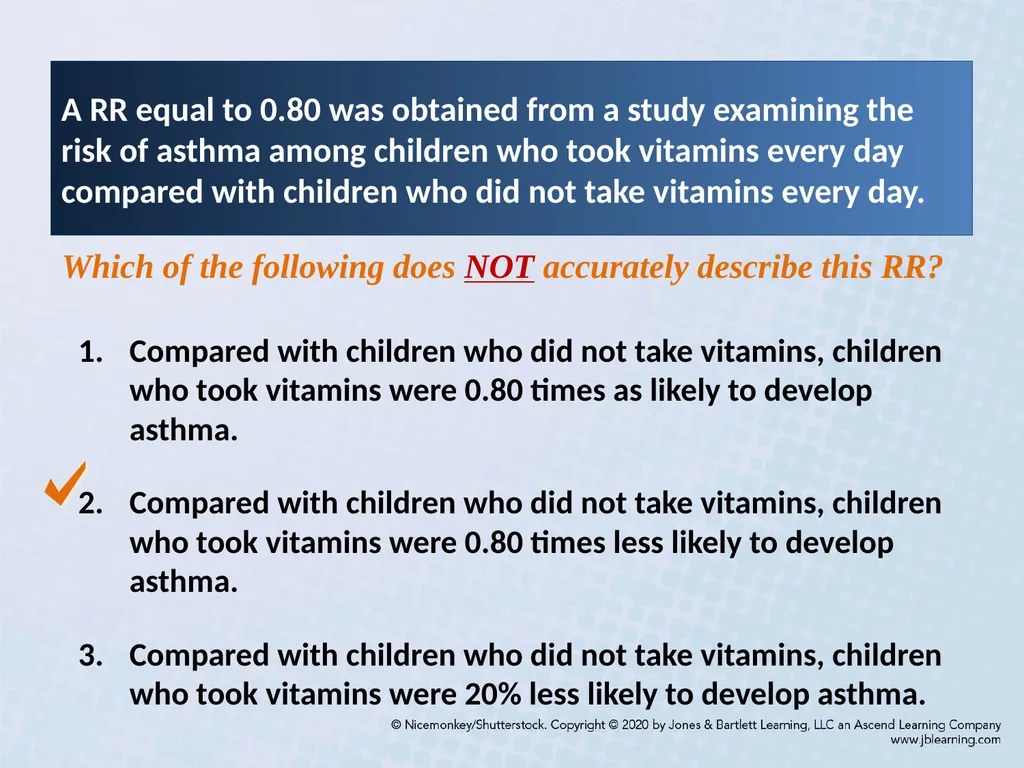
A RR equal to 0.80 was obtained from a study examining the risk of asthma among children who took vitamins every day compared with children who did not take vitamins every day. Which of the following does NOT accurately describe this RR? Compared with children who did not take vitamins, children who took vitamins were 0.80 times as likely to develop asthma.
Compared with children who did not take vitamins, children who took vitamins were 0.80 times less likely to develop asthma.
Compared with children who did not take vitamins, children who took vitamins were 20% less likely to develop asthma.<br>
Compared with children who did not take vitamins, children who took vitamins were 0.80 times less likely to develop asthma.
Compared with children who did not take vitamins, children who took vitamins were 20% less likely to develop asthma.<br>
58
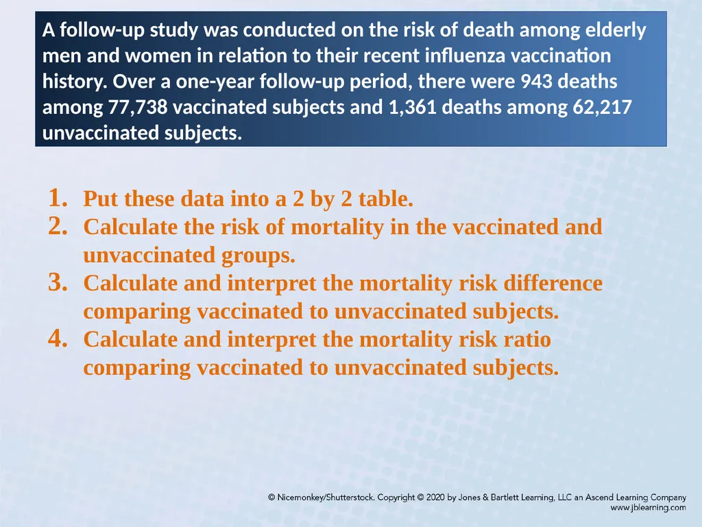
A follow-up study was conducted on the risk of death among elderly men and women in relation to their recent influenza vaccination history. Over a one-year follow-up period, there were 943 deaths among 77,738 vaccinated subjects and 1,361 deaths among 62,217 unvaccinated subjects. Put these data into a 2 by 2 table.
Calculate the risk of mortality in the vaccinated and unvaccinated groups.
Calculate and interpret the mortality risk difference comparing vaccinated to unvaccinated subjects.
Calculate and interpret the mortality risk ratio comparing vaccinated to unvaccinated subjects.<br>
Calculate the risk of mortality in the vaccinated and unvaccinated groups.
Calculate and interpret the mortality risk difference comparing vaccinated to unvaccinated subjects.
Calculate and interpret the mortality risk ratio comparing vaccinated to unvaccinated subjects.<br>
59
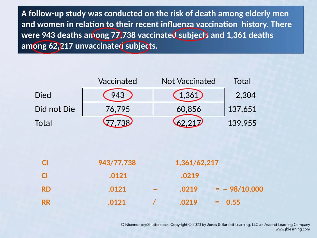
CI .0121 .0219 RD .0121 – .0219 = – 98/10,000 A follow-up study was conducted on the risk of death among elderly men and women in relation to their recent influenza vaccination history. There were 943 deaths among 77,738 vaccinated subjects and 1,361 deaths among 62,217 unvaccinated subjects. RR .0121 / .0219 = 0.55 CI 943/77,738 1,361/62,217<br>
60
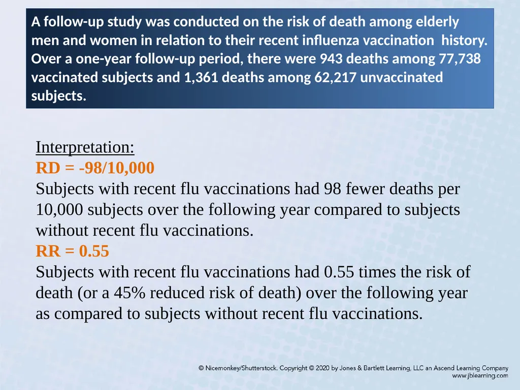
A follow-up study was conducted on the risk of death among elderly men and women in relation to their recent influenza vaccination history. Over a one-year follow-up period, there were 943 deaths among 77,738 vaccinated subjects and 1,361 deaths among 62,217 unvaccinated subjects. Interpretation:
RD = -98/10,000
Subjects with recent flu vaccinations had 98 fewer deaths per 10,000 subjects over the following year compared to subjects without recent flu vaccinations.
RR = 0.55
Subjects with recent flu vaccinations had 0.55 times the risk of death (or a 45% reduced risk of death) over the following year as compared to subjects without recent flu vaccinations.<br>
RD = -98/10,000
Subjects with recent flu vaccinations had 98 fewer deaths per 10,000 subjects over the following year compared to subjects without recent flu vaccinations.
RR = 0.55
Subjects with recent flu vaccinations had 0.55 times the risk of death (or a 45% reduced risk of death) over the following year as compared to subjects without recent flu vaccinations.<br>