CISE301_Topic2 KFUPM 1 CISE301: Numerical Methods

slide1. CISE301_Topic2 KFUPM 1 CISE301: Numerical MethodsTopic 2: Solution of Nonlinear Equations Lectures 5-11: KFUPM

Read Chapters 5 and 6 of the textbook<br>
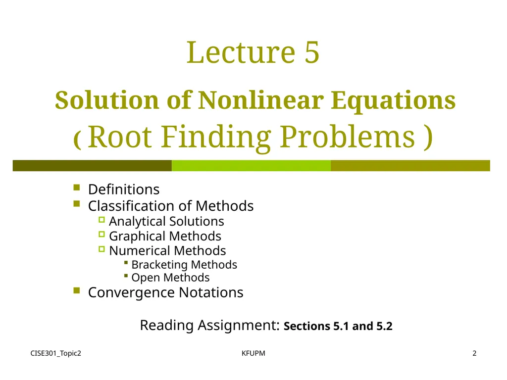
slide2. CISE301_Topic2 KFUPM 2 Lecture 5 Solution of Nonlinear Equations ( Root Finding Problems ) Definitions
Classification of Methods
Analytical Solutions
Graphical Methods
Numerical Methods
Bracketing Methods
Open Methods
Convergence Notations

Reading Assignment: Sections 5.1 and 5.2<br>
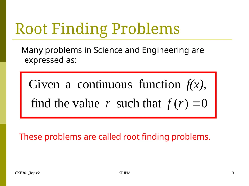
slide3. CISE301_Topic2 KFUPM 3 Root Finding Problems Many problems in Science and Engineering are expressed as: These problems are called root finding problems.<br>
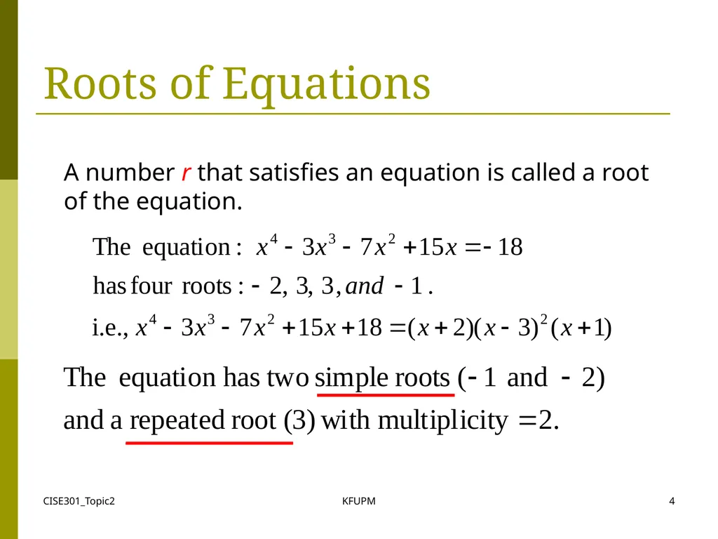
slide4. CISE301_Topic2 KFUPM 4 Roots of Equations A number r that satisfies an equation is called a root of the equation.<br>
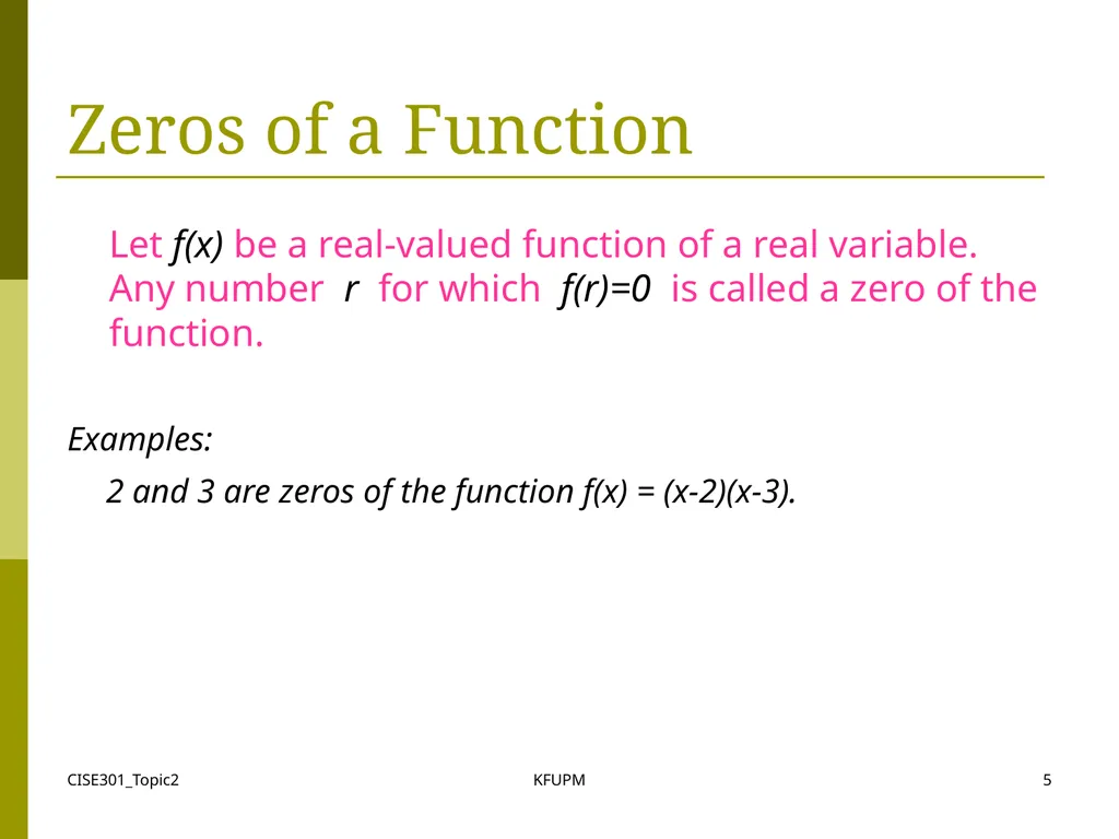
slide5. CISE301_Topic2 KFUPM 5 Zeros of a Function Let f(x) be a real-valued function of a real variable. Any number r for which f(r)=0 is called a zero of the function.

Examples:
2 and 3 are zeros of the function f(x) = (x-2)(x-3).<br>
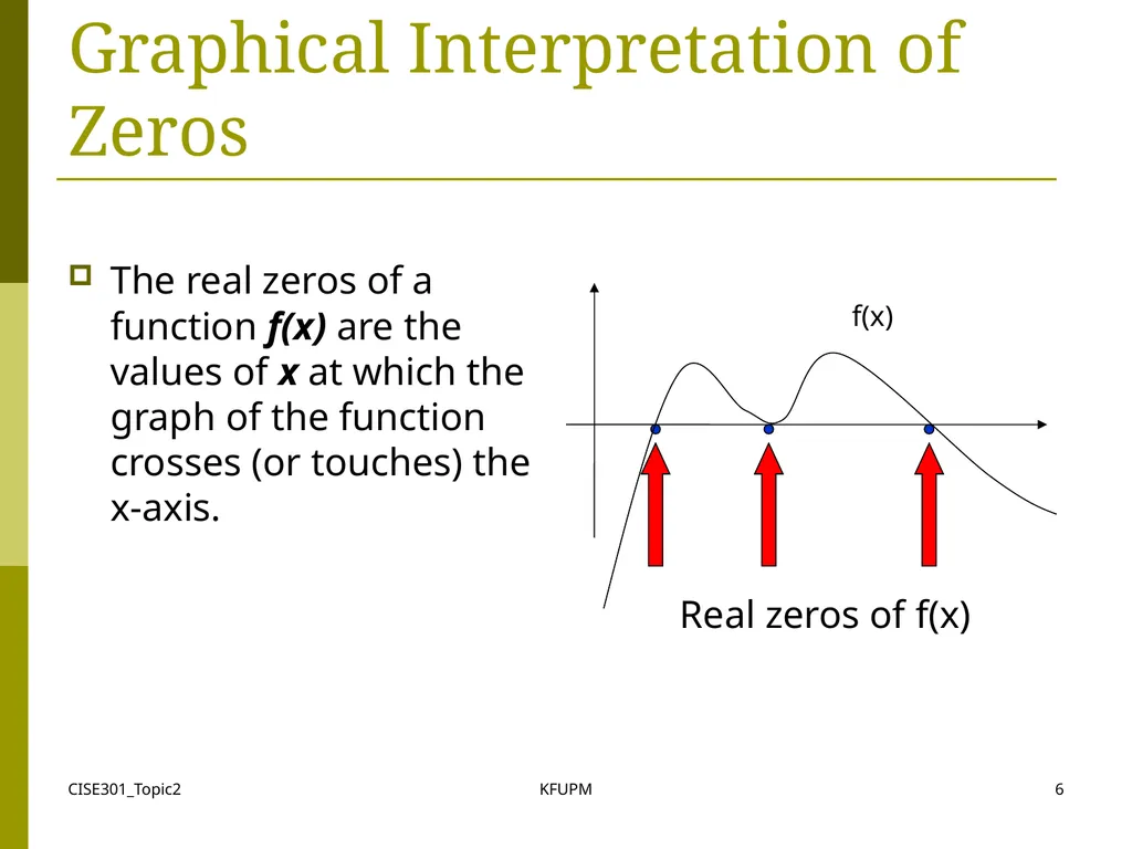
slide6. CISE301_Topic2 KFUPM 6 Graphical Interpretation of Zeros The real zeros of a function f(x) are the values of x at which the graph of the function crosses (or touches) the x-axis. Real zeros of f(x) f(x)<br>
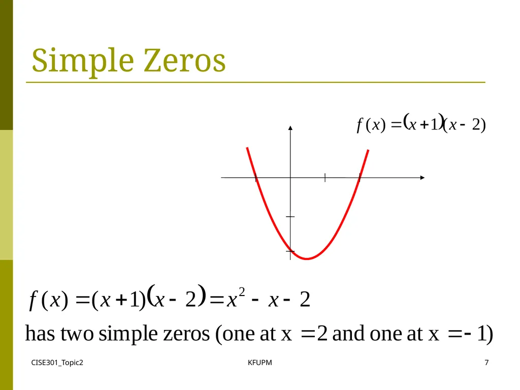
slide7. CISE301_Topic2 KFUPM 7 Simple Zeros<br>
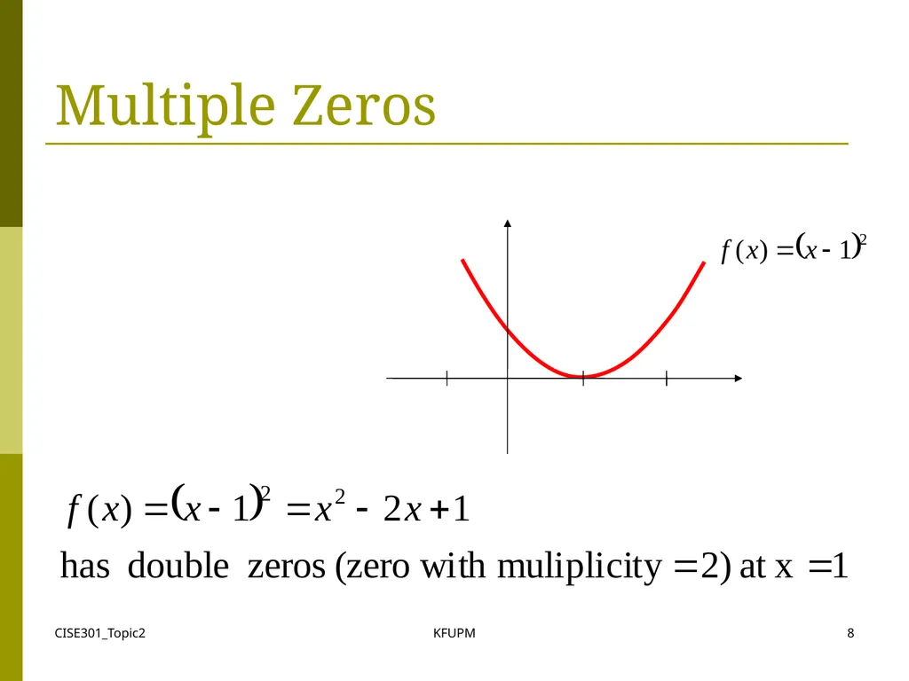
slide8. CISE301_Topic2 KFUPM 8 Multiple Zeros<br>
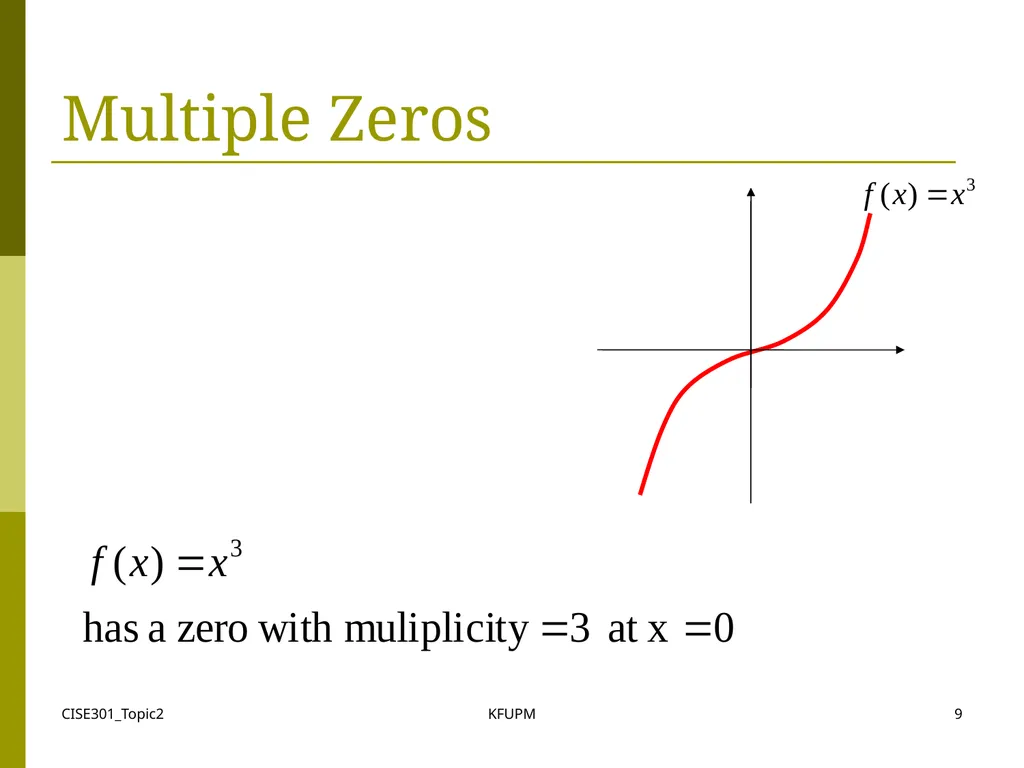
slide9. CISE301_Topic2 KFUPM 9 Multiple Zeros<br>
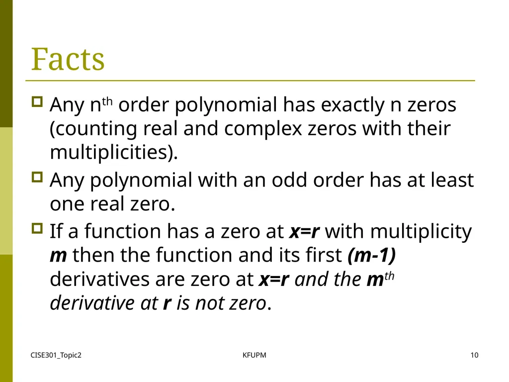
slide10. CISE301_Topic2 KFUPM 10 Facts Any nth order polynomial has exactly n zeros (counting real and complex zeros with their multiplicities).
Any polynomial with an odd order has at least one real zero.
If a function has a zero at x=r with multiplicity m then the function and its first (m-1) derivatives are zero at x=r and the mth derivative at r is not zero.<br>
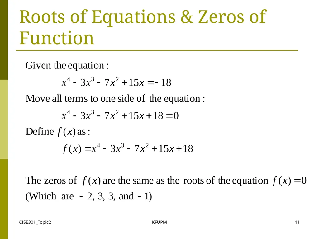
slide11. CISE301_Topic2 KFUPM 11 Roots of Equations & Zeros of Function<br>
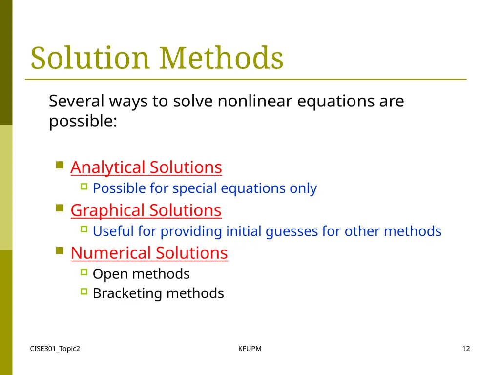
slide12. CISE301_Topic2 KFUPM 12 Solution Methods Several ways to solve nonlinear equations are possible:

Analytical Solutions
Possible for special equations only
Graphical Solutions
Useful for providing initial guesses for other methods
Numerical Solutions
Open methods
Bracketing methods<br>
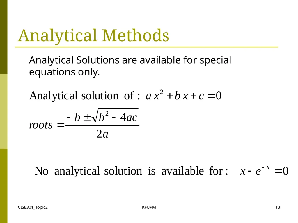
slide13. CISE301_Topic2 KFUPM 13 Analytical Methods Analytical Solutions are available for special equations only.<br>
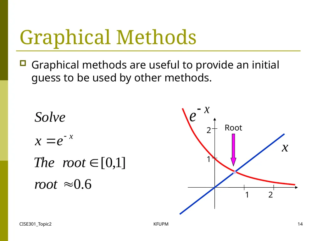
slide14. CISE301_Topic2 KFUPM 14 Graphical Methods Graphical methods are useful to provide an initial guess to be used by other methods. Root 1 2 2

1<br>
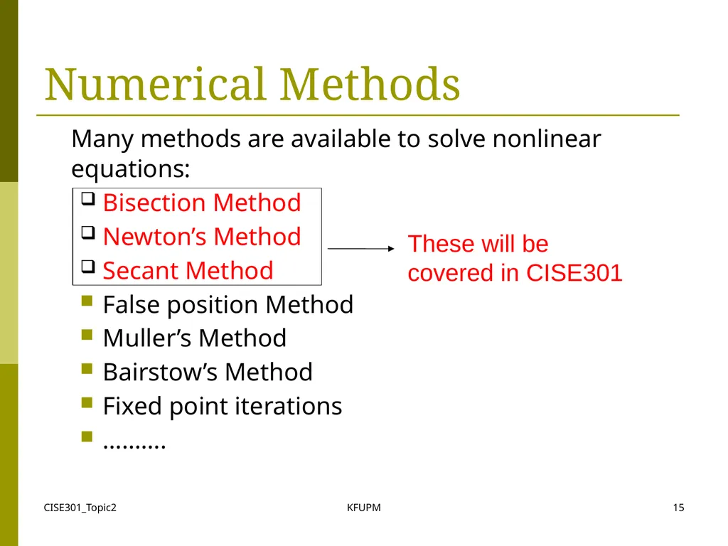
slide15. CISE301_Topic2 KFUPM 15 Numerical Methods Many methods are available to solve nonlinear equations:
Bisection Method
Newton’s Method
Secant Method
False position Method
Muller’s Method
Bairstow’s Method
Fixed point iterations
………. These will be covered in CISE301<br>
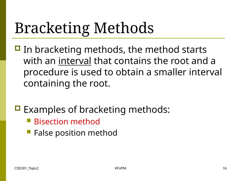
slide16. CISE301_Topic2 KFUPM 16 Bracketing Methods In bracketing methods, the method starts with an interval that contains the root and a procedure is used to obtain a smaller interval containing the root.

Examples of bracketing methods:
Bisection method
False position method<br>
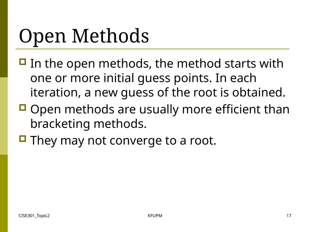
slide17. CISE301_Topic2 KFUPM 17 Open Methods In the open methods, the method starts with one or more initial guess points. In each iteration, a new guess of the root is obtained.
Open methods are usually more efficient than bracketing methods.
They may not converge to a root.<br>
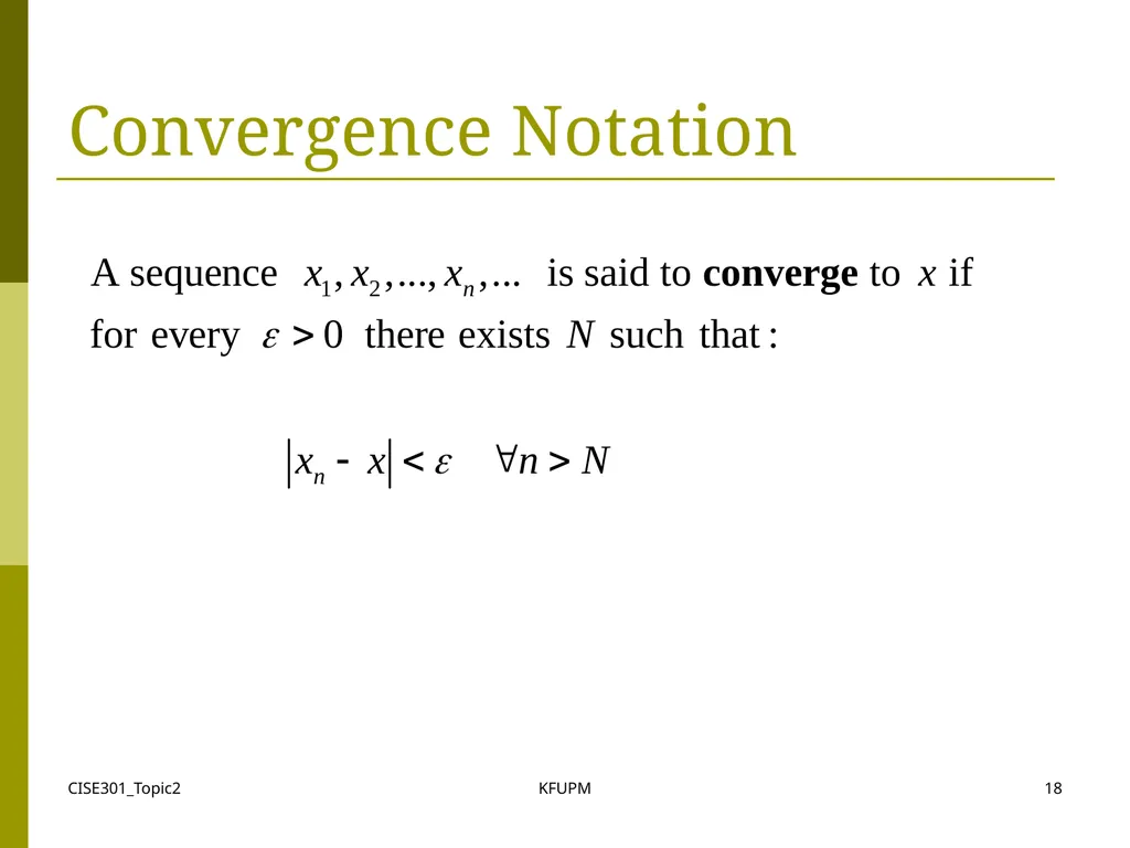
slide18. CISE301_Topic2 KFUPM 18 Convergence Notation<br>
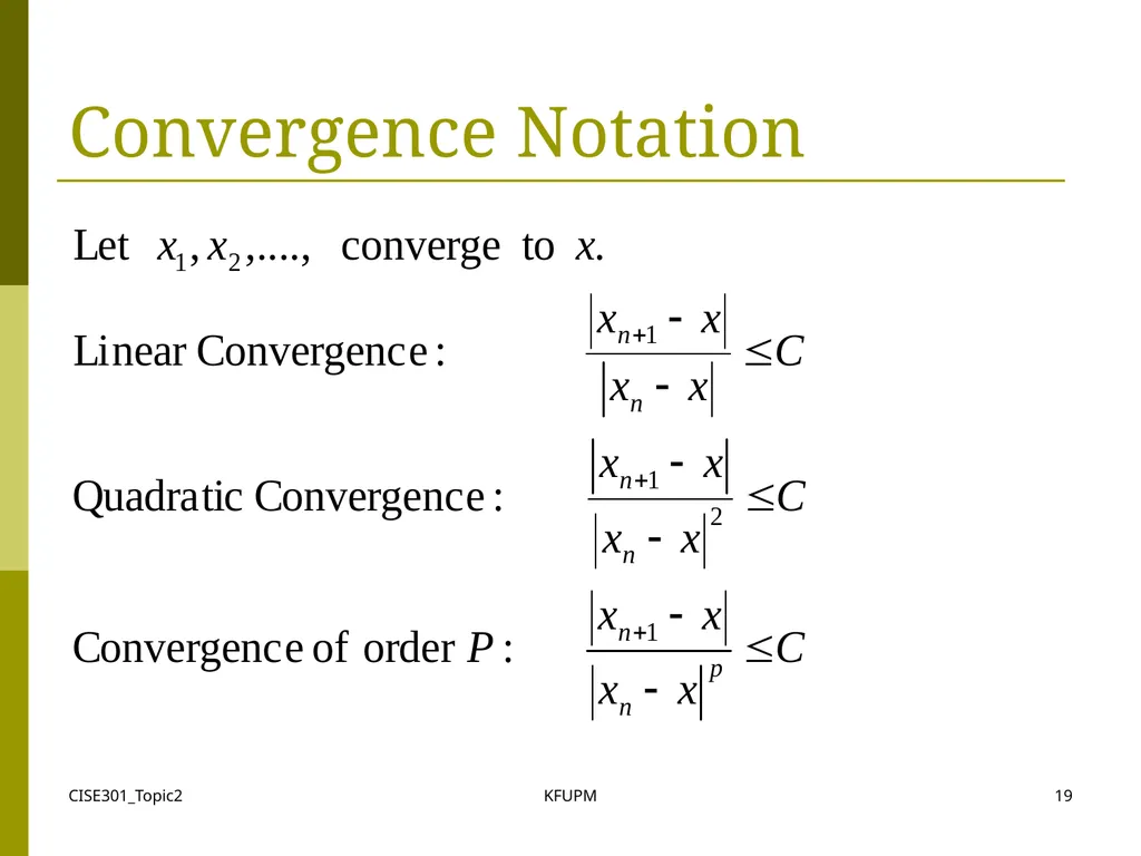
slide19. CISE301_Topic2 KFUPM 19 Convergence Notation<br>
slide20. CISE301_Topic2 KFUPM 20 Speed of Convergence We can compare different methods in terms of their convergence rate.
Quadratic convergence is faster than linear convergence.
A method with convergence order q converges faster than a method with convergence order p if q>p.
Methods of convergence order p>1 are said to have super linear convergence.<br>
slide21. CISE301_Topic2 KFUPM 21 Lectures 6-7Bisection Method The Bisection Algorithm
Convergence Analysis of Bisection Method
Examples

Reading Assignment: Sections 5.1 and 5.2<br>
slide22. CISE301_Topic2 KFUPM 22 Introduction The Bisection method is one of the simplest methods to find a zero of a nonlinear function.
It is also called interval halving method.
To use the Bisection method, one needs an initial interval that is known to contain a zero of the function.
The method systematically reduces the interval. It does this by dividing the interval into two equal parts, performs a simple test and based on the result of the test, half of the interval is thrown away.
The procedure is repeated until the desired interval size is obtained.<br>
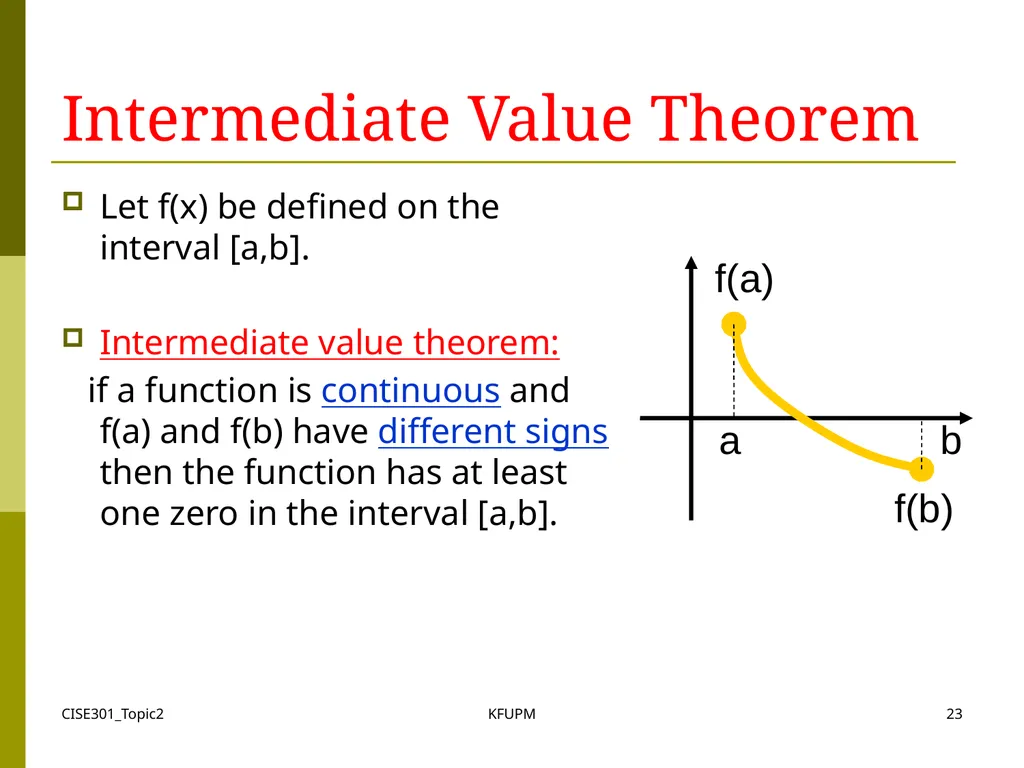
slide23. CISE301_Topic2 KFUPM 23 Intermediate Value Theorem Let f(x) be defined on the interval [a,b].

Intermediate value theorem:
if a function is continuous and f(a) and f(b) have different signs then the function has at least one zero in the interval [a,b]. a b f(a) f(b)<br>
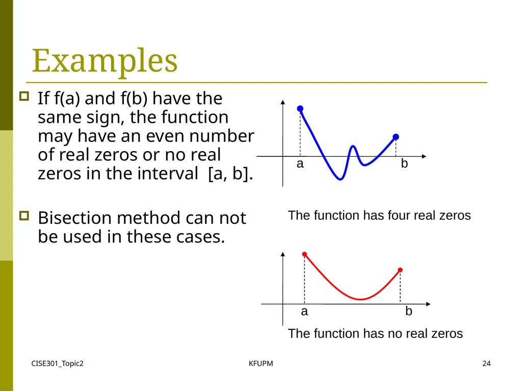
slide24. CISE301_Topic2 KFUPM 24 Examples If f(a) and f(b) have the same sign, the function may have an even number of real zeros or no real zeros in the interval [a, b].

Bisection method can not be used in these cases. a b a b The function has four real zeros The function has no real zeros<br>
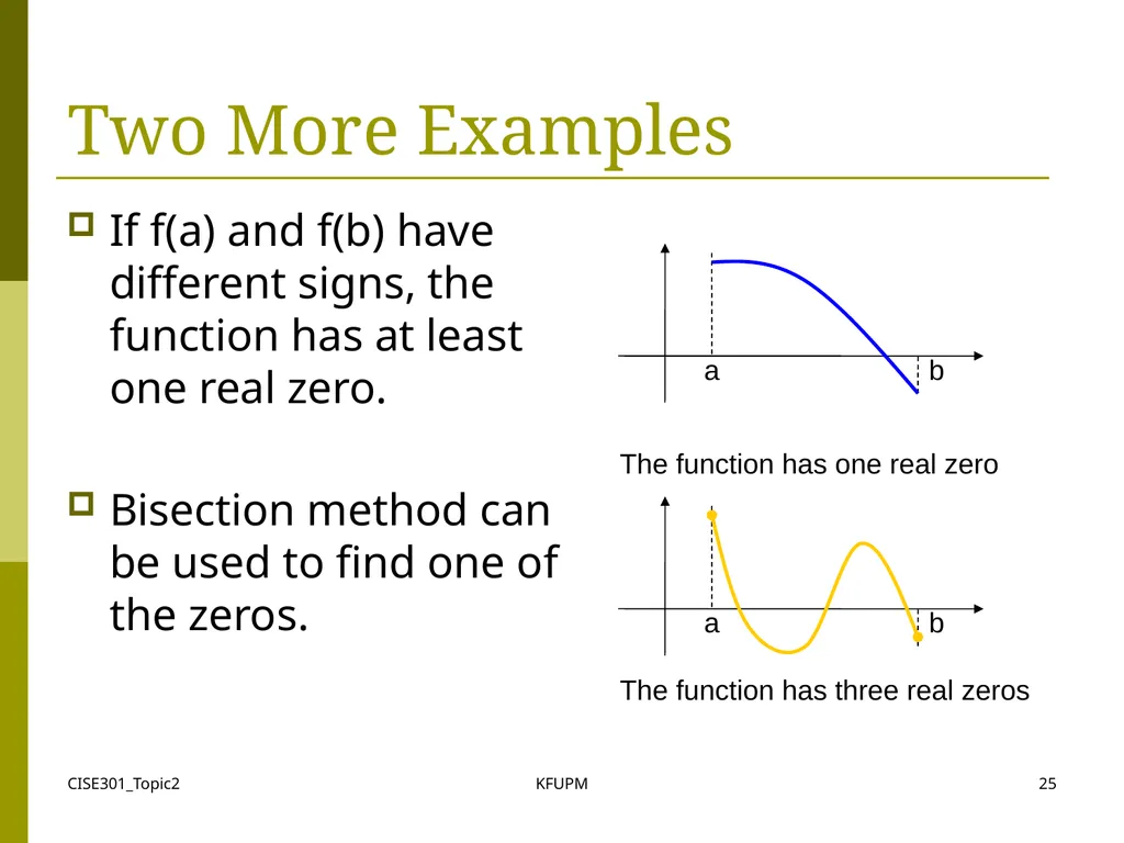
slide25. CISE301_Topic2 KFUPM 25 Two More Examples a b a b If f(a) and f(b) have different signs, the function has at least one real zero.

Bisection method can be used to find one of the zeros. The function has one real zero The function has three real zeros<br>
slide26. CISE301_Topic2 KFUPM 26 Bisection Method If the function is continuous on [a,b] and f(a) and f(b) have different signs, Bisection method obtains a new interval that is half of the current interval and the sign of the function at the end points of the interval are different.

This allows us to repeat the Bisection procedure to further reduce the size of the interval.<br>
slide27. CISE301_Topic2 KFUPM 27 Bisection Method Assumptions:
Given an interval [a,b]
f(x) is continuous on [a,b]
f(a) and f(b) have opposite signs.

These assumptions ensure the existence of at least one zero in the interval [a,b] and the bisection method can be used to obtain a smaller interval that contains the zero.<br>
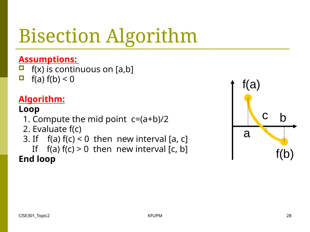
slide28. CISE301_Topic2 KFUPM 28 Bisection Algorithm Assumptions:
f(x) is continuous on [a,b]
f(a) f(b) < 0

Algorithm:
Loop
1. Compute the mid point c=(a+b)/2
2. Evaluate f(c)
3. If f(a) f(c) < 0 then new interval [a, c]
If f(a) f(c) > 0 then new interval [c, b]
End loop a b f(a) f(b) c<br>
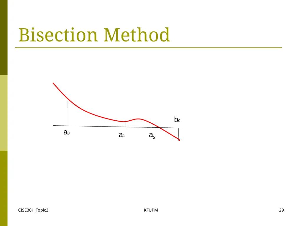
slide29. CISE301_Topic2 KFUPM 29 Bisection Method a0 b0 a1 a2<br>
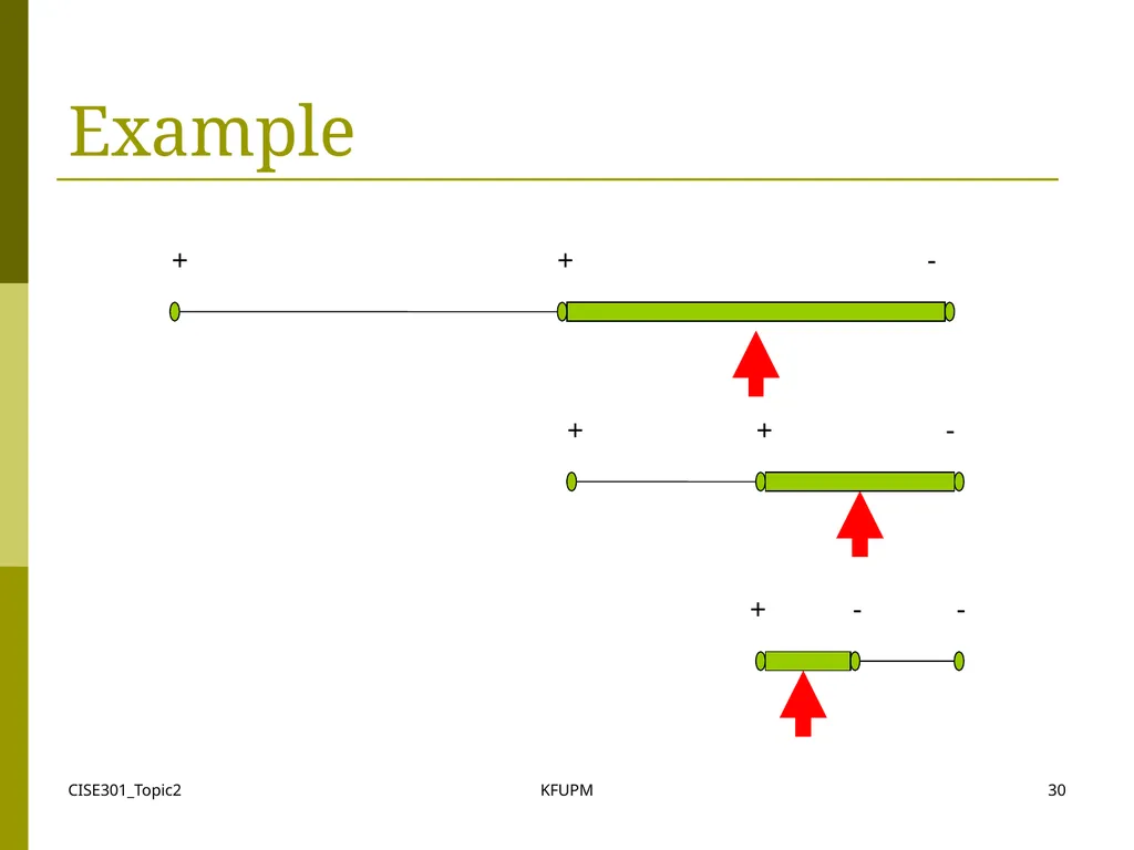
slide30. CISE301_Topic2 KFUPM 30 Example + + - + + - + - -<br>
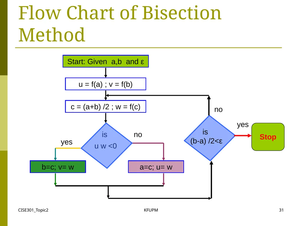
slide31. CISE301_Topic2 KFUPM 31 Flow Chart of Bisection Method Start: Given a,b and ε u = f(a) ; v = f(b) c = (a+b) /2 ; w = f(c) is
u w <0 a=c; u= w b=c; v= w is
(b-a) /2<ε yes yes no Stop no<br>
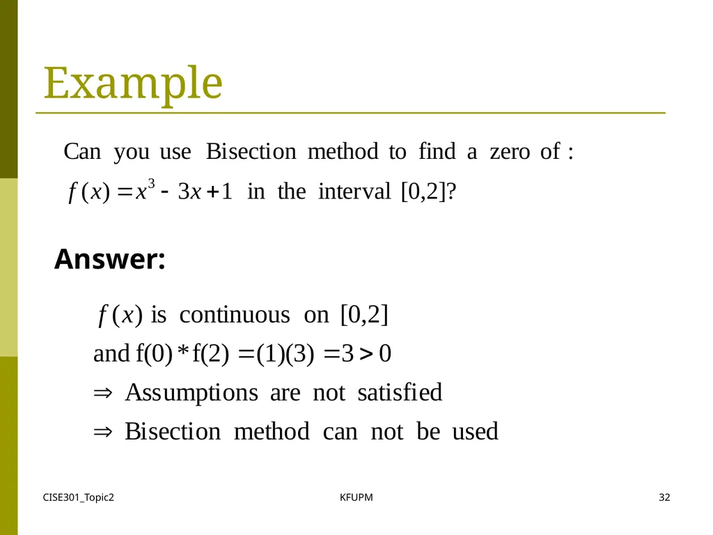
slide32. CISE301_Topic2 KFUPM 32 Example Answer:<br>
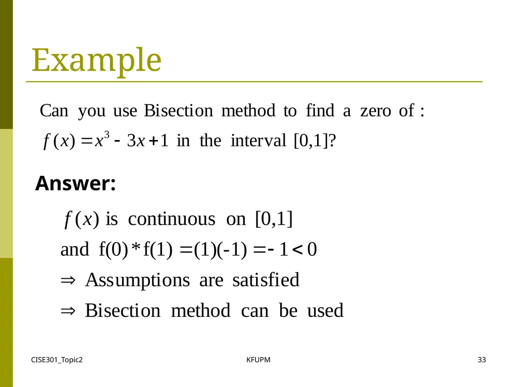
slide33. CISE301_Topic2 KFUPM 33 Example Answer:<br>
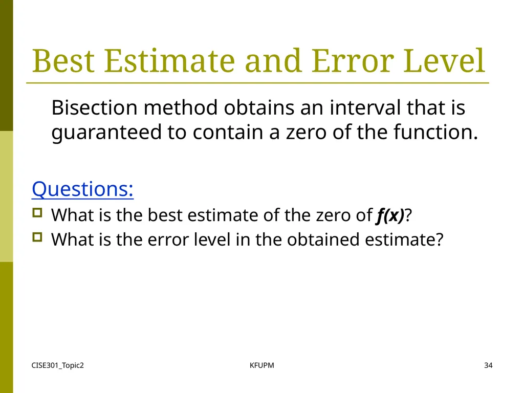
slide34. CISE301_Topic2 KFUPM 34 Best Estimate and Error Level Bisection method obtains an interval that is guaranteed to contain a zero of the function.

Questions:
What is the best estimate of the zero of f(x)?
What is the error level in the obtained estimate?<br>
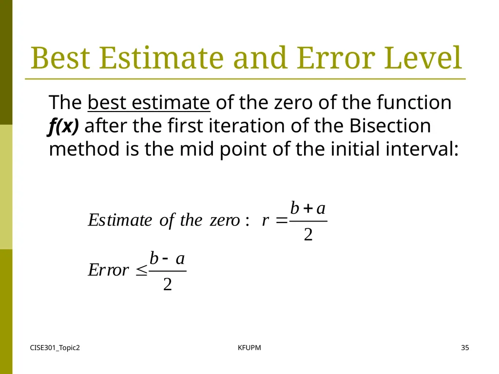
slide35. CISE301_Topic2 KFUPM 35 Best Estimate and Error Level The best estimate of the zero of the function f(x) after the first iteration of the Bisection method is the mid point of the initial interval:<br>
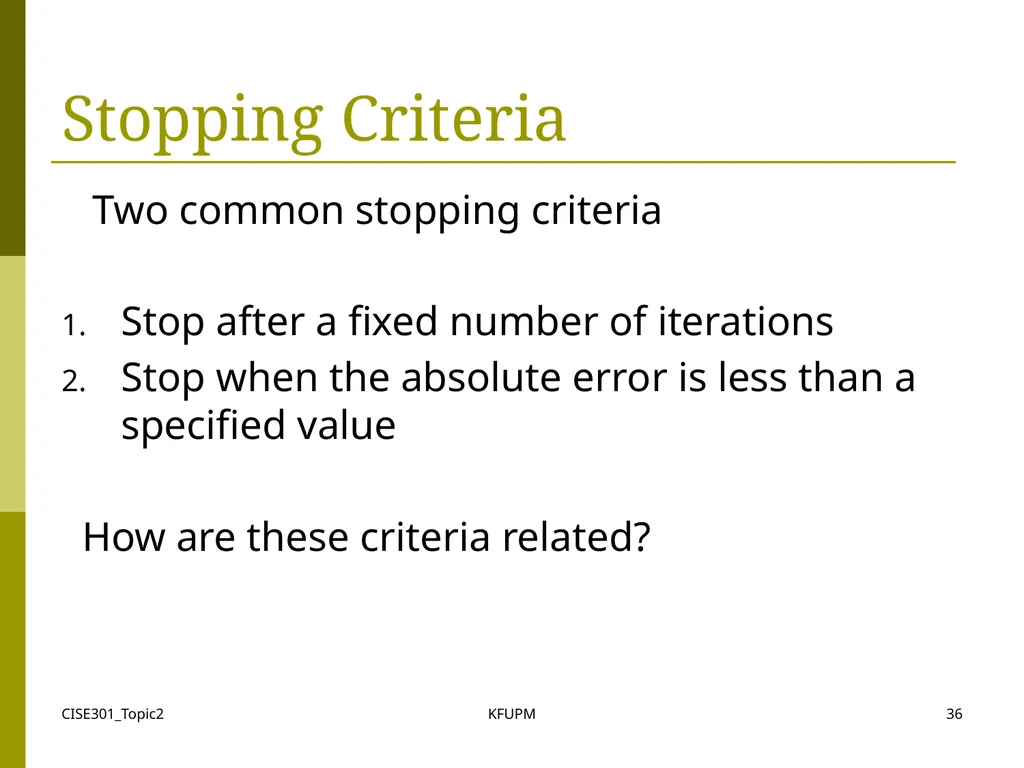
slide36. CISE301_Topic2 KFUPM 36 Stopping Criteria Two common stopping criteria

Stop after a fixed number of iterations
Stop when the absolute error is less than a specified value

How are these criteria related?<br>
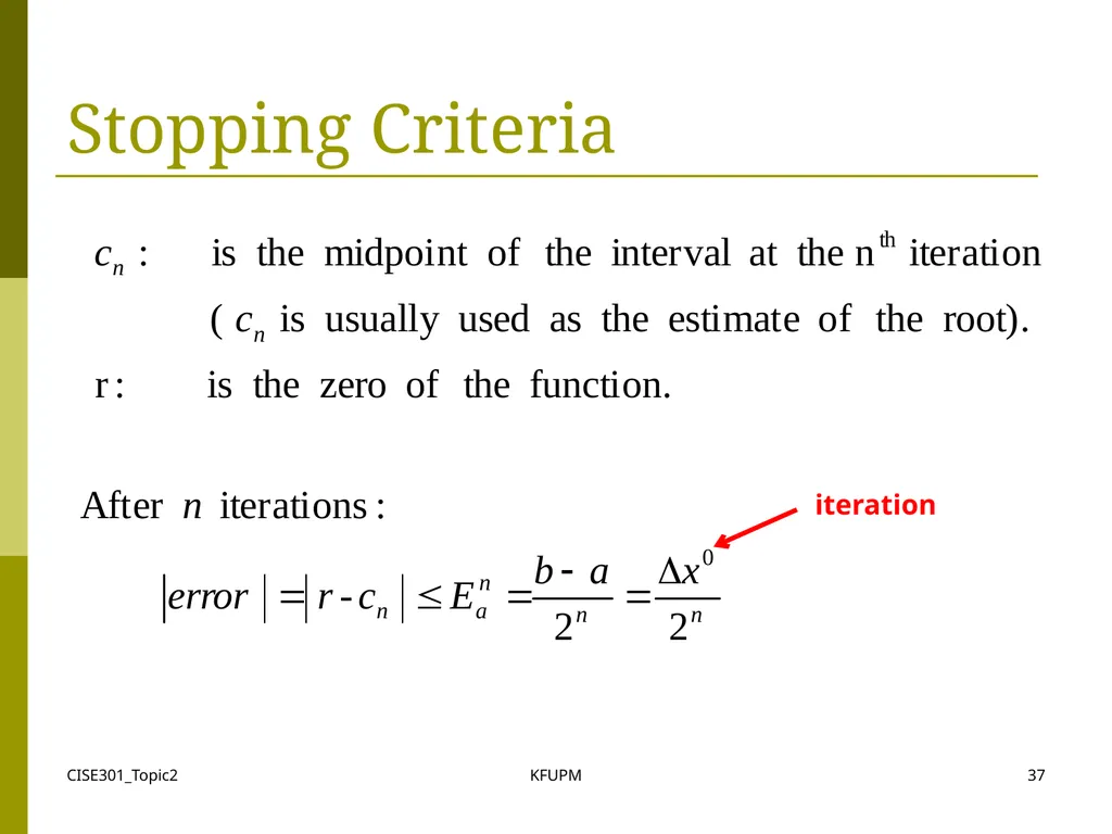
slide37. CISE301_Topic2 KFUPM 37 Stopping Criteria iteration<br>
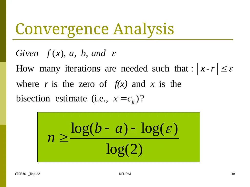
slide38. CISE301_Topic2 KFUPM 38 Convergence Analysis<br>
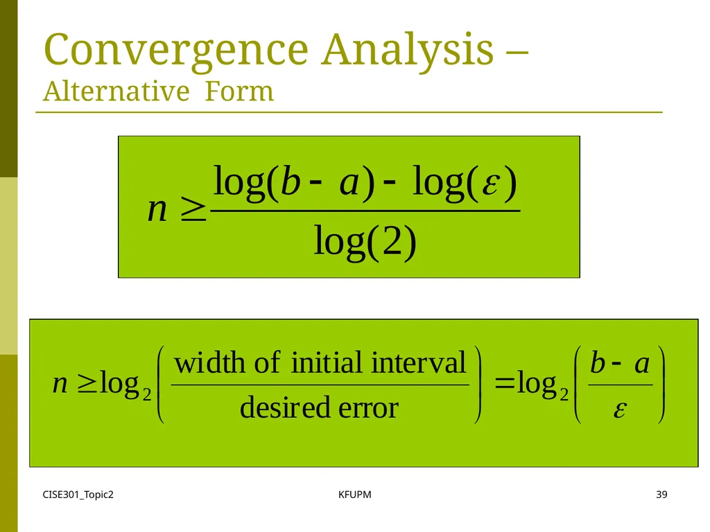
slide39. CISE301_Topic2 KFUPM 39 Convergence Analysis – Alternative Form<br>
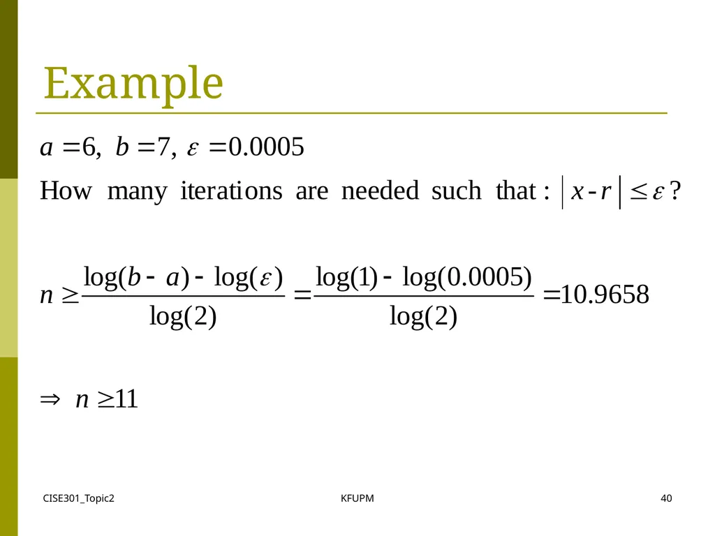
slide40. CISE301_Topic2 KFUPM 40 Example<br>
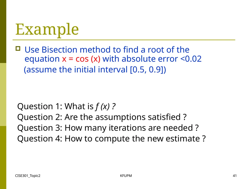
slide41. CISE301_Topic2 KFUPM 41 Example Use Bisection method to find a root of the equation x = cos (x) with absolute error <0.02
(assume the initial interval [0.5, 0.9]) Question 1: What is f (x) ?
Question 2: Are the assumptions satisfied ?
Question 3: How many iterations are needed ?
Question 4: How to compute the new estimate ?<br>
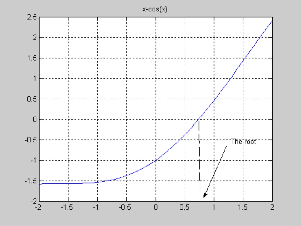
slide42. CISE301_Topic2 KFUPM 42<br>
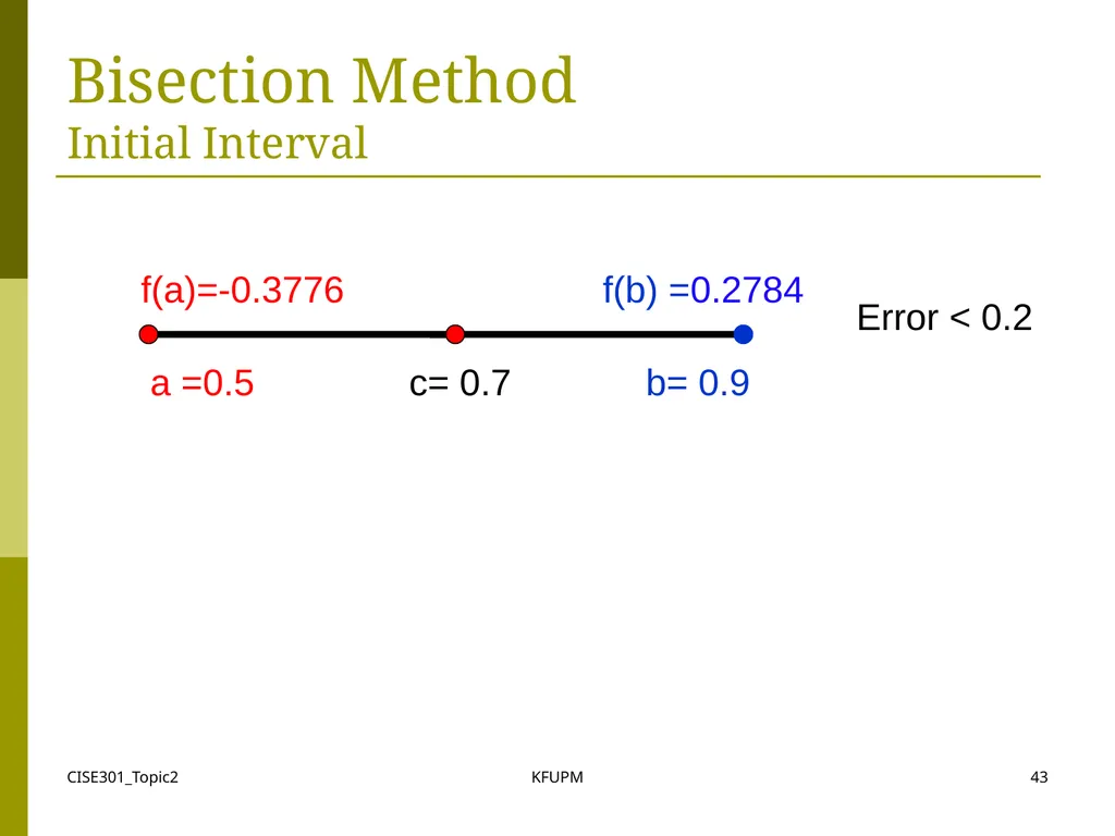
slide43. CISE301_Topic2 KFUPM 43 Bisection MethodInitial Interval a =0.5 c= 0.7 b= 0.9 f(a)=-0.3776 f(b) =0.2784 Error < 0.2<br>
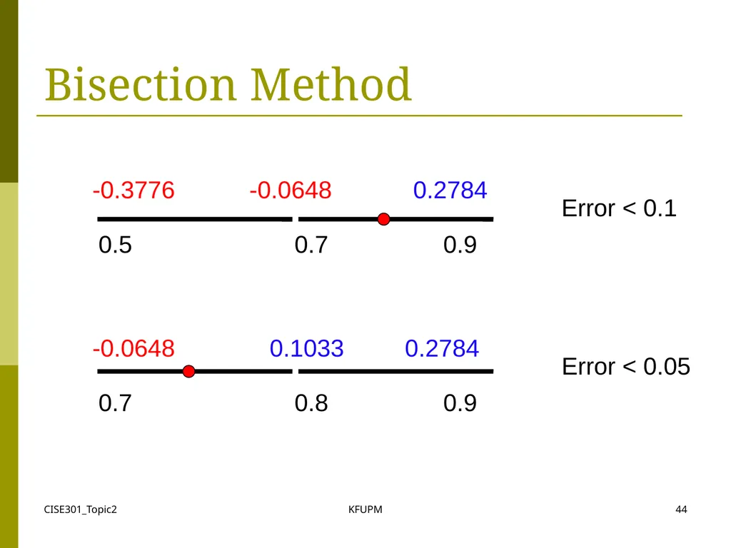
slide44. CISE301_Topic2 KFUPM 44 Bisection Method 0.5 0.7 0.9 -0.3776 -0.0648 0.2784 Error < 0.1 0.7 0.8 0.9 -0.0648 0.1033 0.2784 Error < 0.05<br>
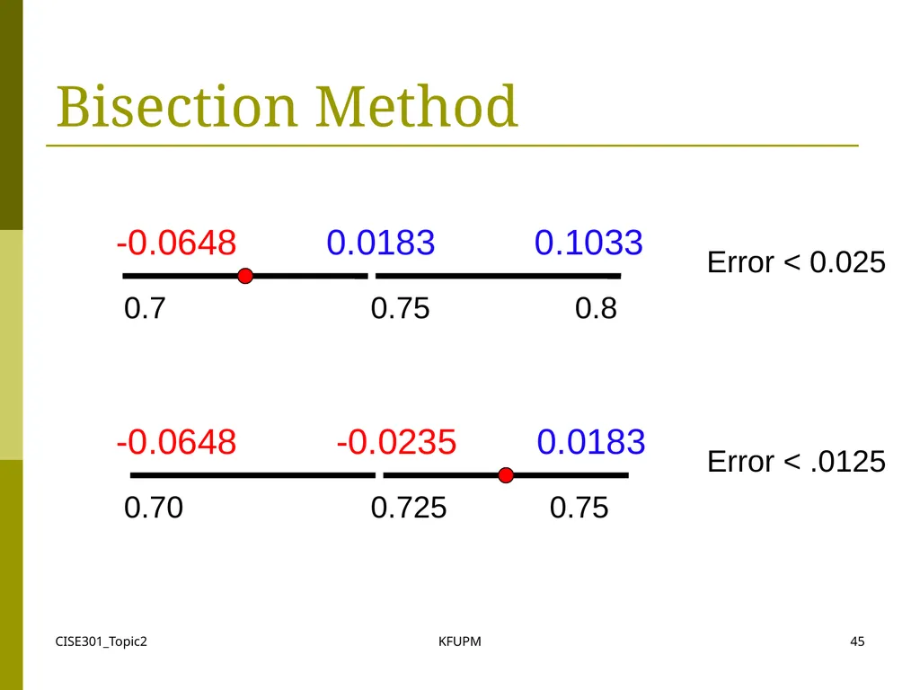
slide45. CISE301_Topic2 KFUPM 45 Bisection Method 0.7 0.75 0.8 -0.0648 0.0183 0.1033 Error < 0.025 0.70 0.725 0.75 -0.0648 -0.0235 0.0183 Error < .0125<br>
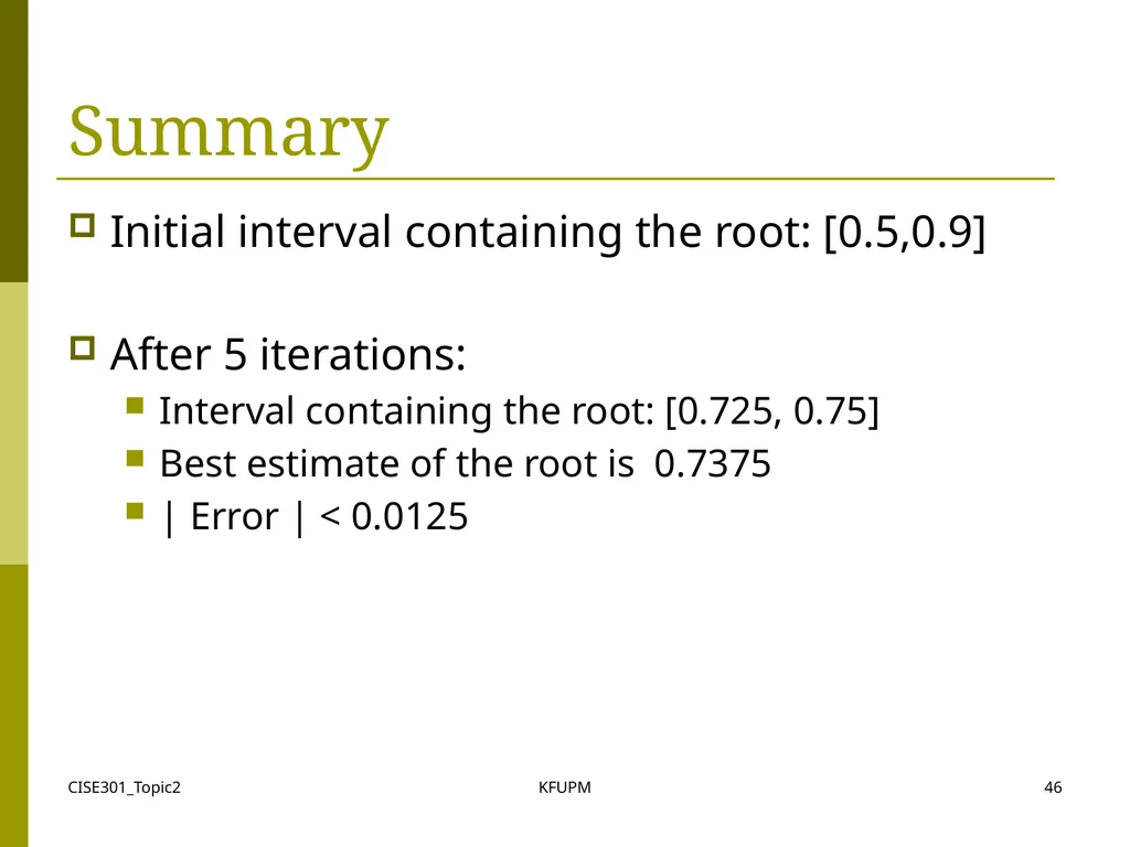
slide46. CISE301_Topic2 KFUPM 46 Summary Initial interval containing the root: [0.5,0.9]

After 5 iterations:
Interval containing the root: [0.725, 0.75]
Best estimate of the root is 0.7375
| Error | < 0.0125<br>
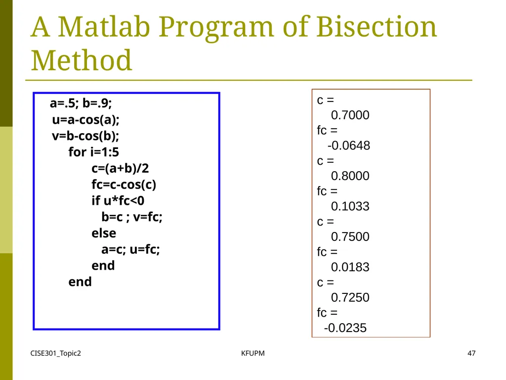
slide47. CISE301_Topic2 KFUPM 47 A Matlab Program of Bisection Method a=.5; b=.9;
u=a-cos(a);
v=b-cos(b);
for i=1:5
c=(a+b)/2
fc=c-cos(c)
if u*fc<0
b=c ; v=fc;
else
a=c; u=fc;
end
end c =
0.7000
fc =
-0.0648
c =
0.8000
fc =
0.1033
c =
0.7500
fc =
0.0183
c =
0.7250
fc =
-0.0235<br>
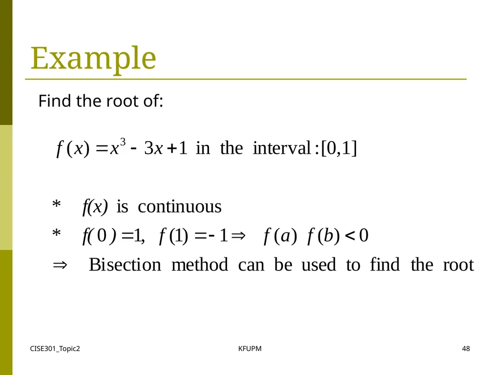
slide48. CISE301_Topic2 KFUPM 48 Example Find the root of:<br>
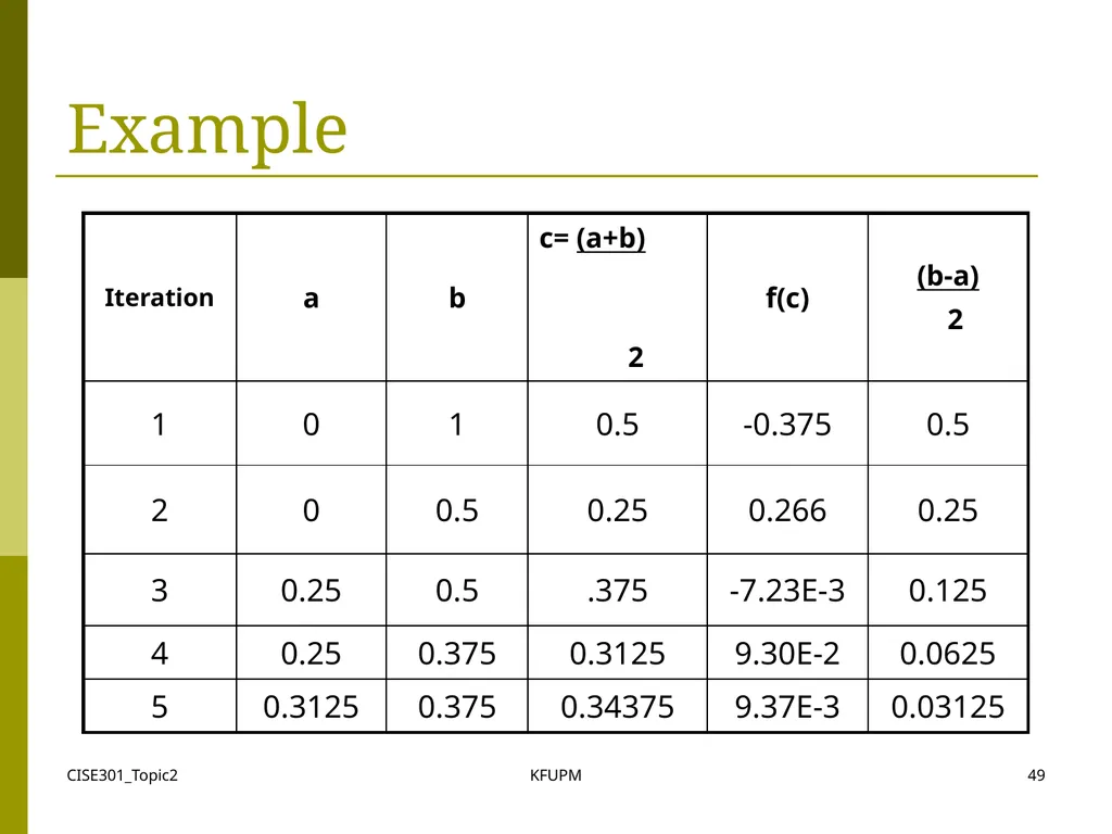
slide49. CISE301_Topic2 KFUPM 49 Example<br>
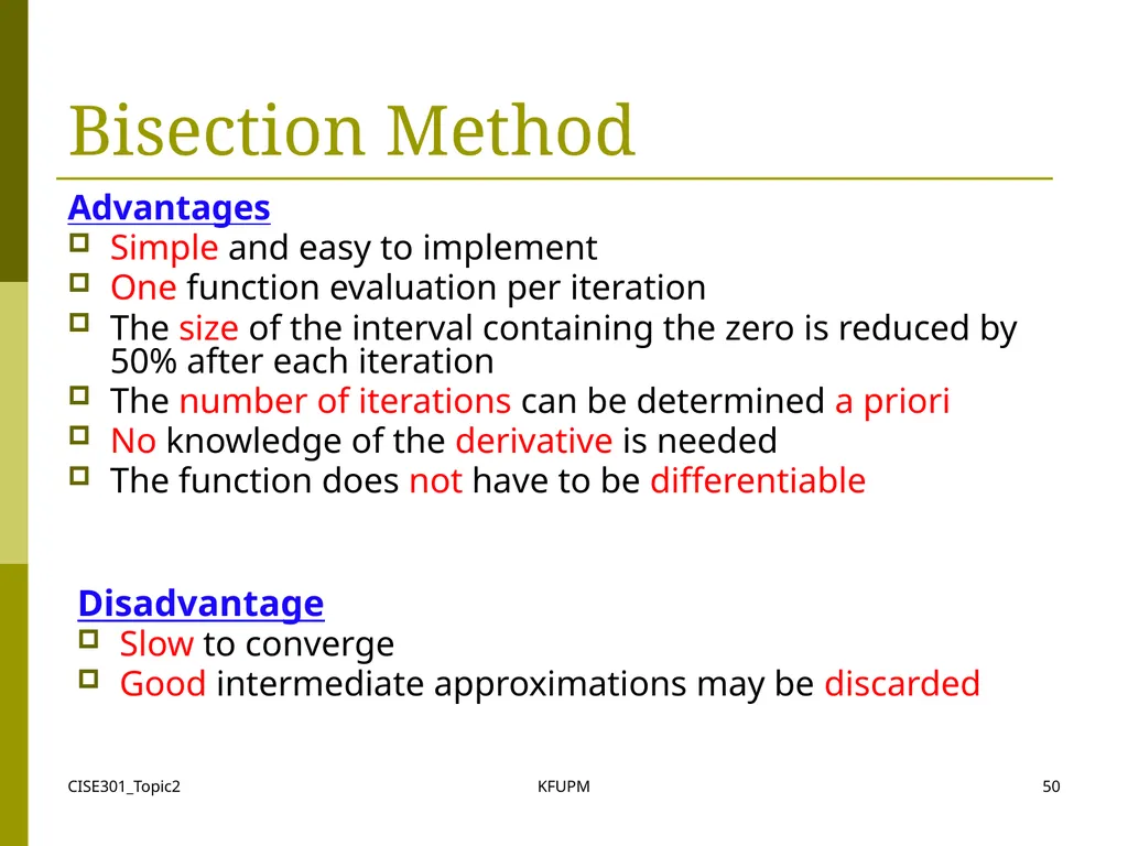
slide50. CISE301_Topic2 KFUPM 50 Bisection Method Advantages
Simple and easy to implement
One function evaluation per iteration
The size of the interval containing the zero is reduced by 50% after each iteration
The number of iterations can be determined a priori
No knowledge of the derivative is needed
The function does not have to be differentiable Disadvantage
Slow to converge
Good intermediate approximations may be discarded<br>
slide51. CISE301_Topic2 KFUPM 51 Lecture 8-9 Newton-Raphson Method Assumptions
Interpretation
Examples
Convergence Analysis<br>
slide52. CISE301_Topic2 KFUPM 52 Newton-Raphson Method (Also known as Newton’s Method) Given an initial guess of the root x0, Newton-Raphson method uses information about the function and its derivative at that point to find a better guess of the root.

Assumptions:
f(x) is continuous and the first derivative is known
An initial guess x0 such that f’(x0)≠0 is given<br>
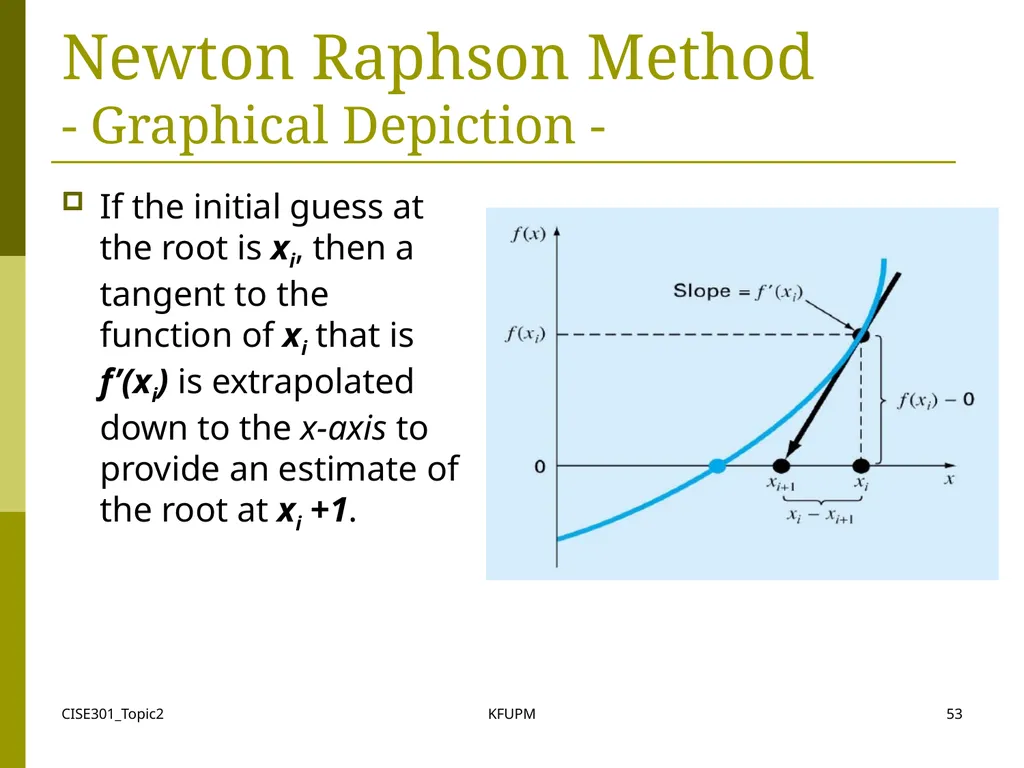
slide53. CISE301_Topic2 KFUPM 53 Newton Raphson Method- Graphical Depiction - If the initial guess at the root is xi, then a tangent to the function of xi that is f’(xi) is extrapolated down to the x-axis to provide an estimate of the root at xi +1.<br>
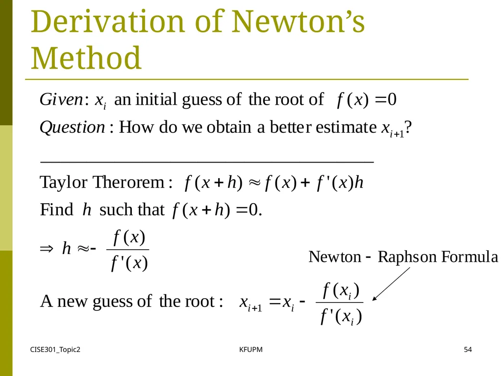
slide54. CISE301_Topic2 KFUPM 54 Derivation of Newton’s Method<br>
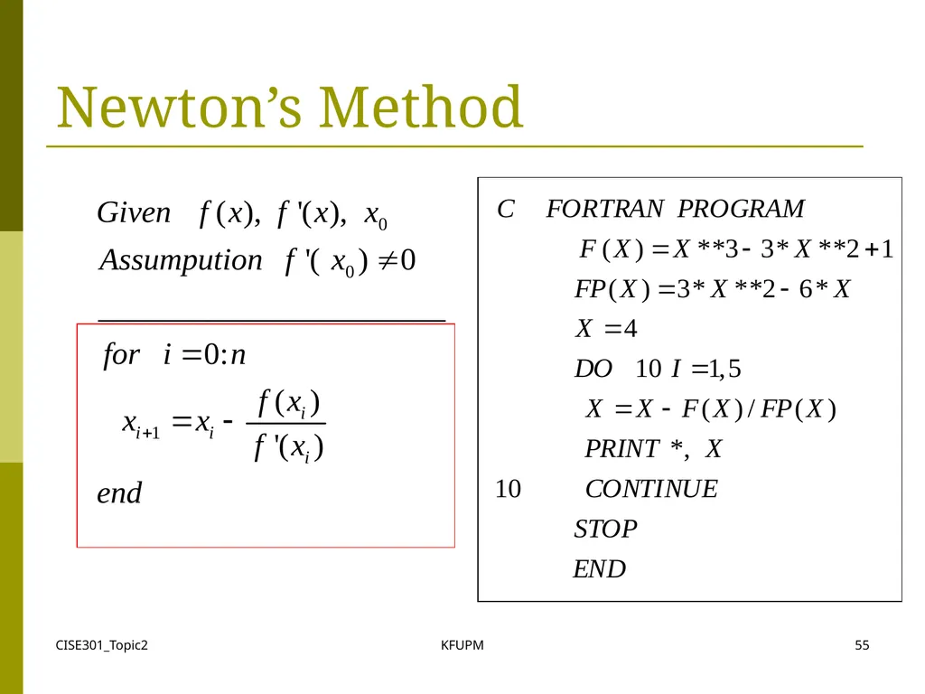
slide55. CISE301_Topic2 KFUPM 55 Newton’s Method<br>
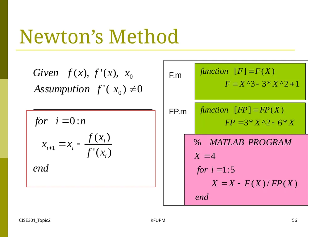
slide56. CISE301_Topic2 KFUPM 56 Newton’s Method F.m

FP.m<br>
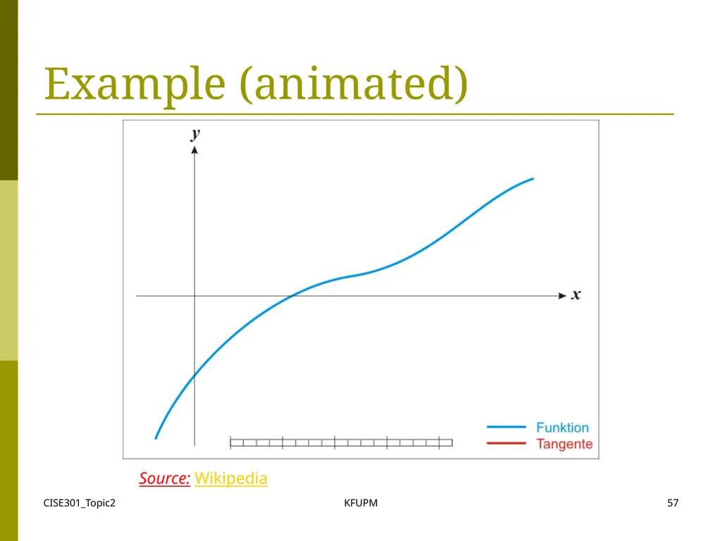
slide57. Example (animated) CISE301_Topic2 KFUPM 57 Source: Wikipedia<br>
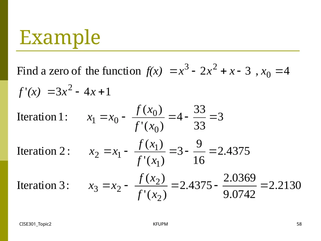
slide58. CISE301_Topic2 KFUPM 58 Example<br>
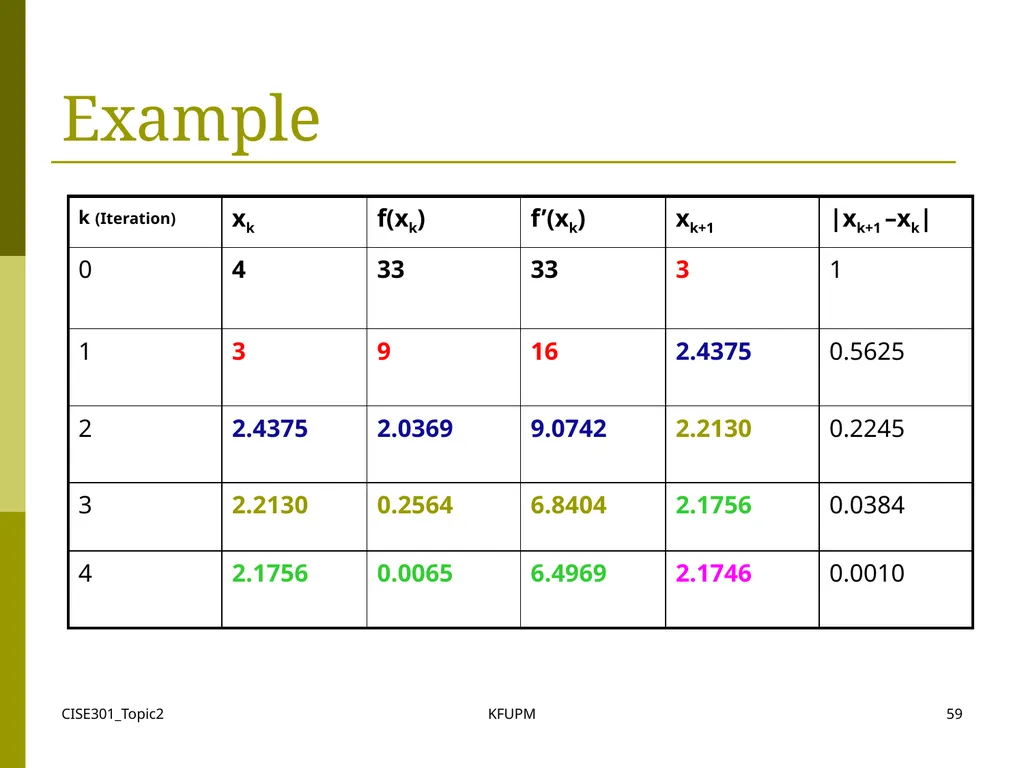
slide59. CISE301_Topic2 KFUPM 59 Example<br>
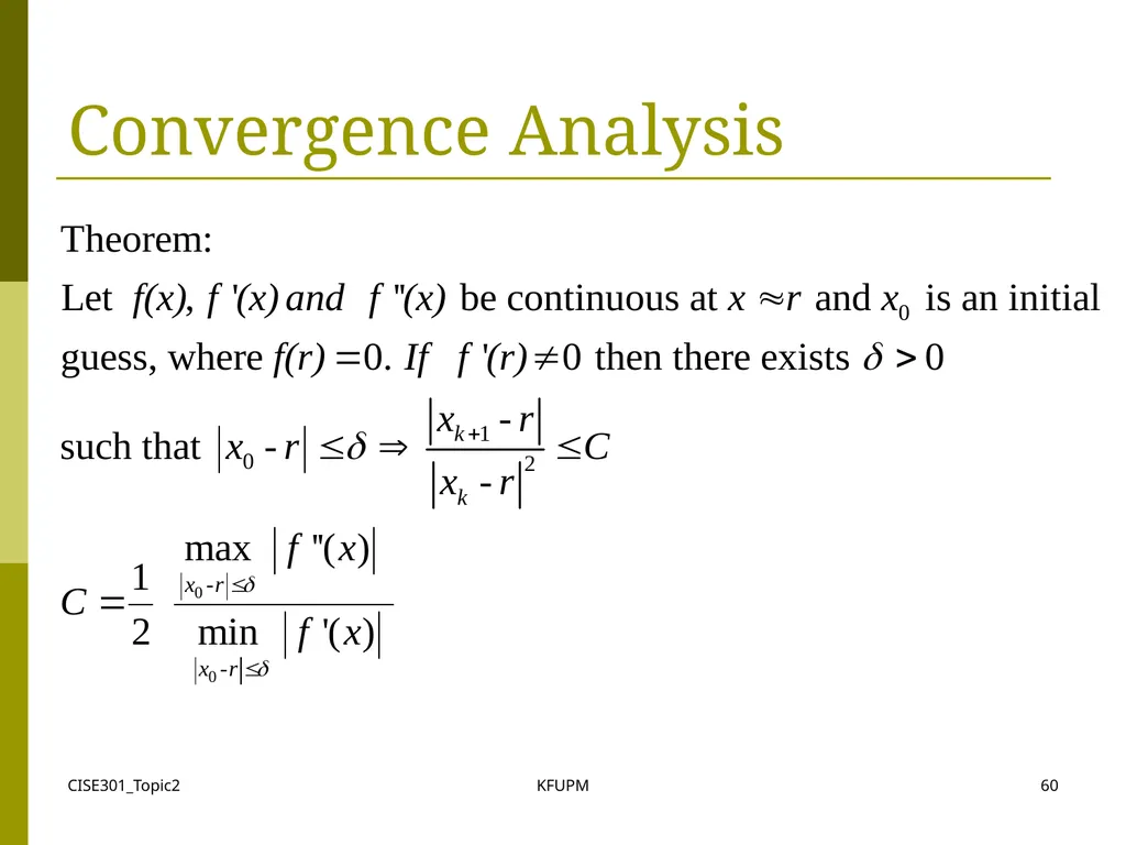
slide60. CISE301_Topic2 KFUPM 60 Convergence Analysis<br>
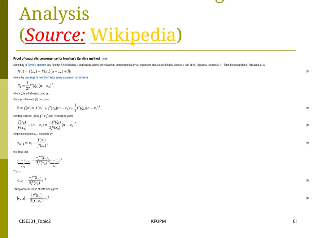
slide61. Formal Proof of Convergence Analysis(Source: Wikipedia) CISE301_Topic2 KFUPM 61<br>
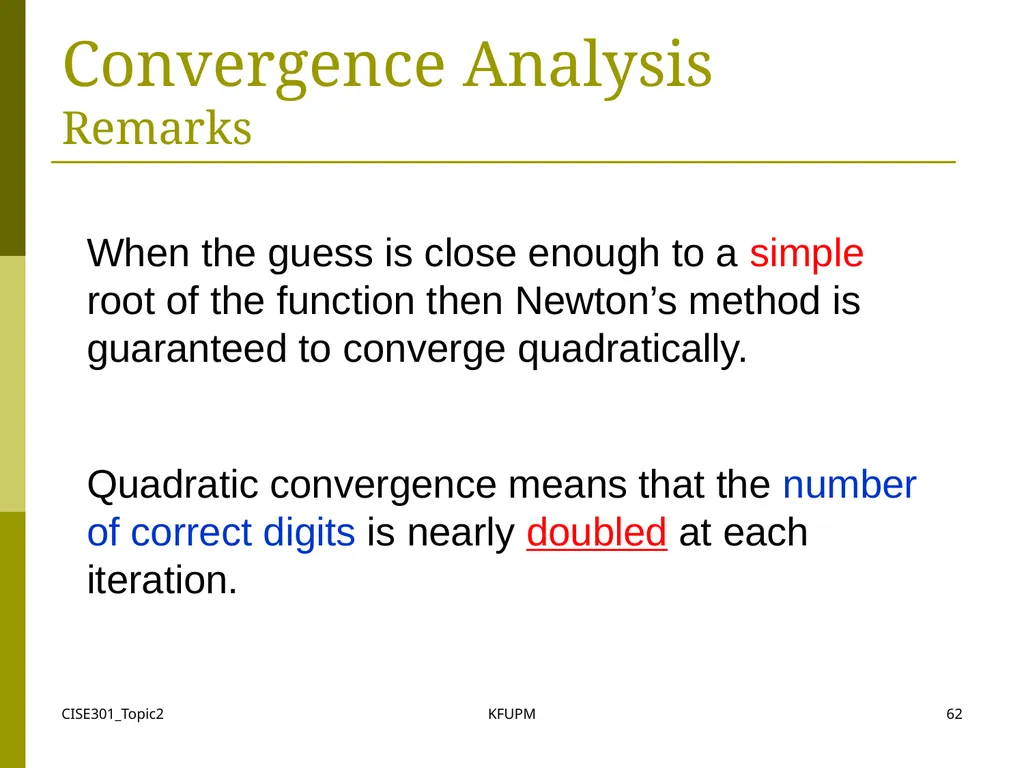
slide62. CISE301_Topic2 KFUPM 62 Convergence AnalysisRemarks When the guess is close enough to a simple root of the function then Newton’s method is guaranteed to converge quadratically.

Quadratic convergence means that the number of correct digits is nearly doubled at each iteration.<br>
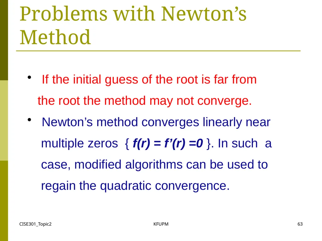
slide63. CISE301_Topic2 KFUPM 63 Problems with Newton’s Method If the initial guess of the root is far from
the root the method may not converge.
Newton’s method converges linearly near
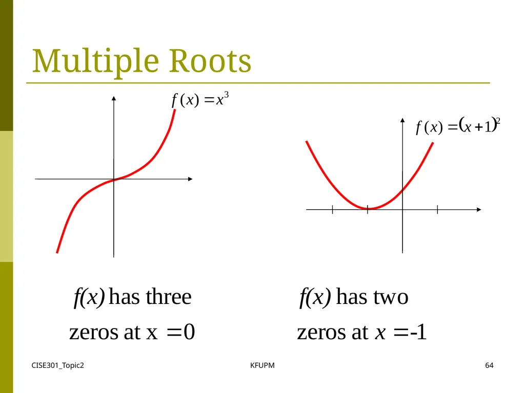
multiple zeros { f(r) = f’(r) =0 }. In such a
case, modified algorithms can be used to
regain the quadratic convergence.<br>
slide64. CISE301_Topic2 KFUPM 64 Multiple Roots<br>
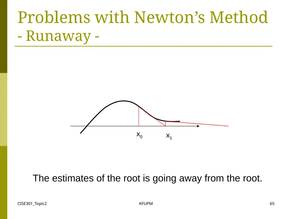
slide65. CISE301_Topic2 KFUPM 65 Problems with Newton’s Method- Runaway - The estimates of the root is going away from the root. x0 x1<br>
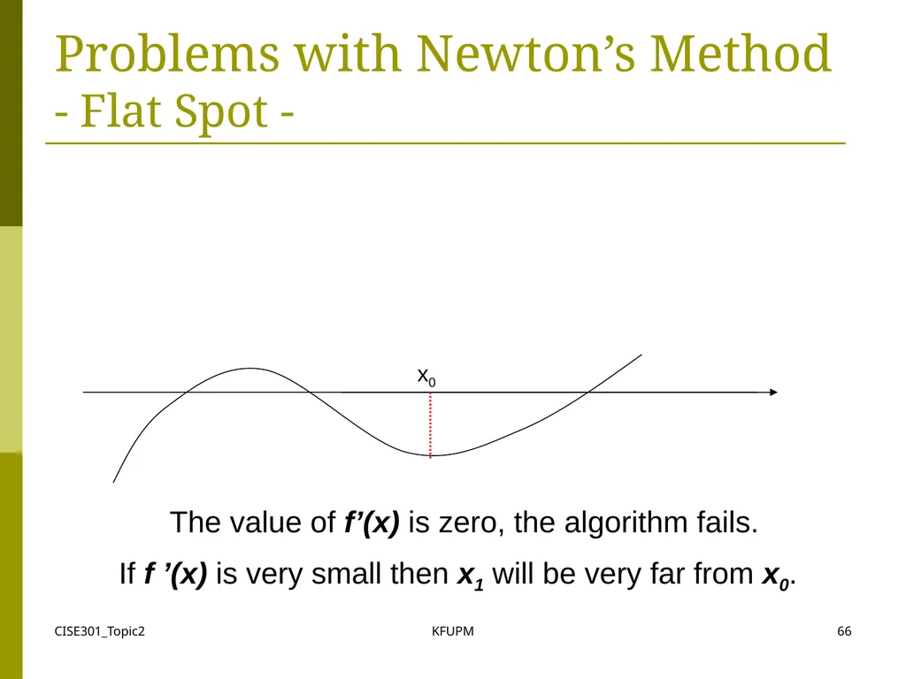
slide66. CISE301_Topic2 KFUPM 66 Problems with Newton’s Method- Flat Spot - The value of f’(x) is zero, the algorithm fails.
If f ’(x) is very small then x1 will be very far from x0. x0<br>
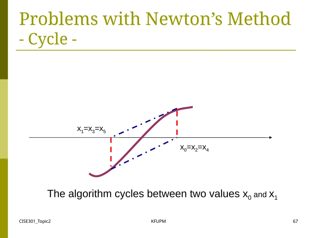
slide67. CISE301_Topic2 KFUPM 67 Problems with Newton’s Method- Cycle - The algorithm cycles between two values x0 and x1 x0=x2=x4 x1=x3=x5<br>
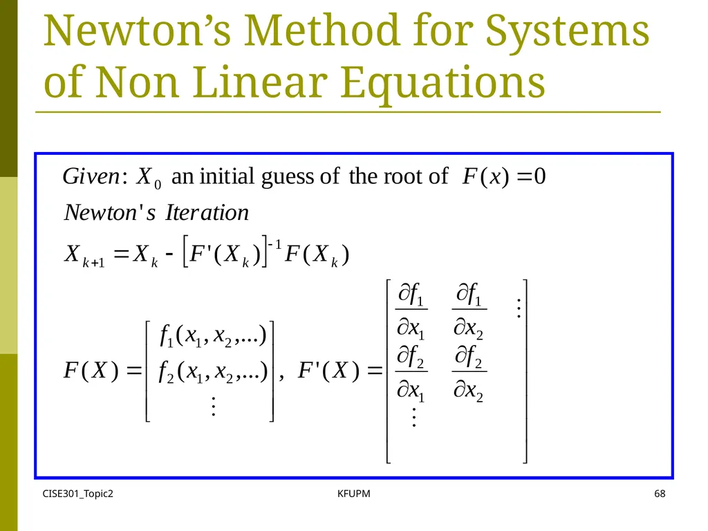
slide68. CISE301_Topic2 KFUPM 68 Newton’s Method for Systems of Non Linear Equations<br>
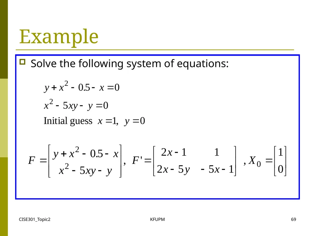
slide69. CISE301_Topic2 KFUPM 69 Example Solve the following system of equations:<br>
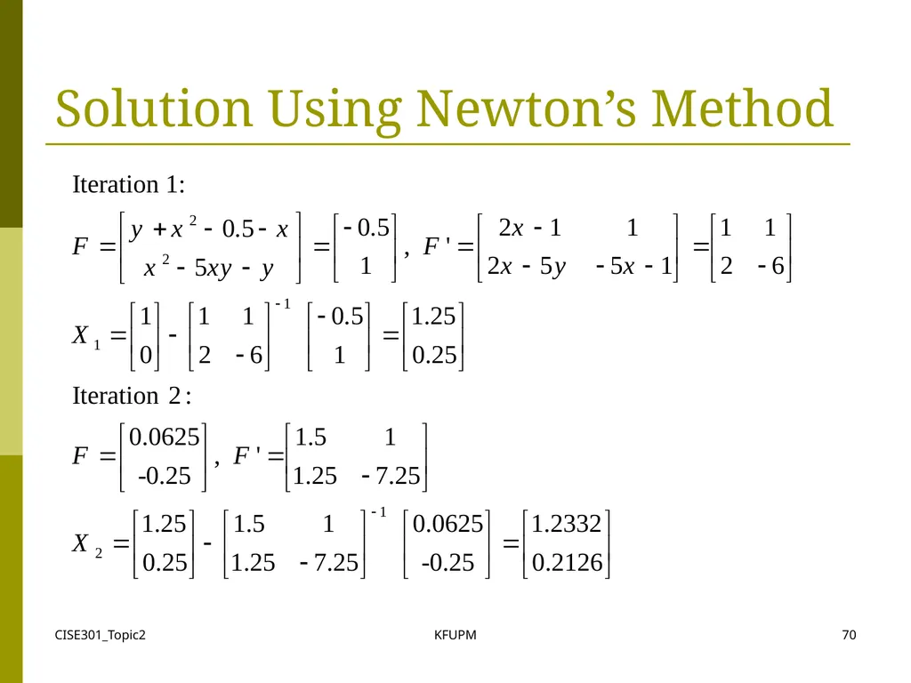
slide70. CISE301_Topic2 KFUPM 70 Solution Using Newton’s Method<br>
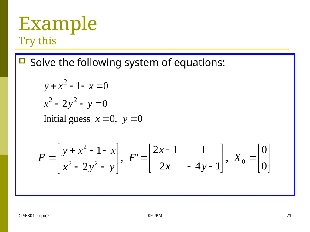
slide71. CISE301_Topic2 KFUPM 71 ExampleTry this Solve the following system of equations:<br>
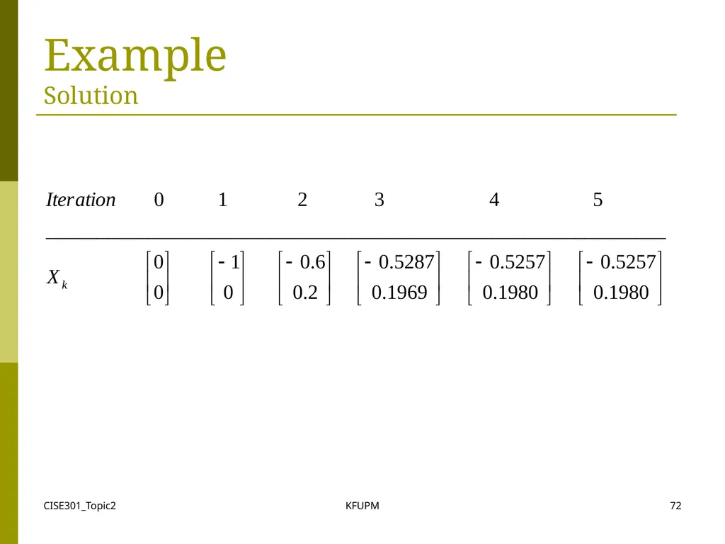
slide72. CISE301_Topic2 KFUPM 72 ExampleSolution<br>
slide73. CISE301_Topic2 KFUPM 73 Lectures 10 Secant Method Secant Method
Examples
Convergence Analysis<br>
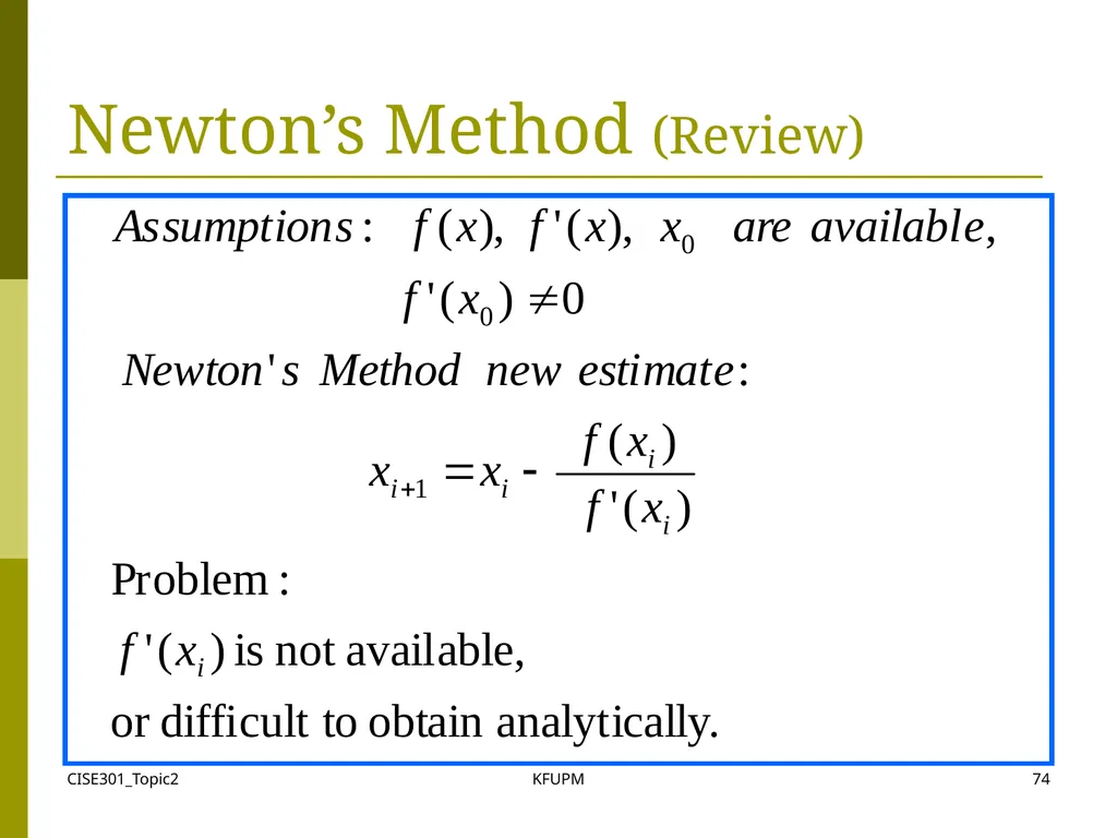
slide74. CISE301_Topic2 KFUPM 74 Newton’s Method (Review)<br>
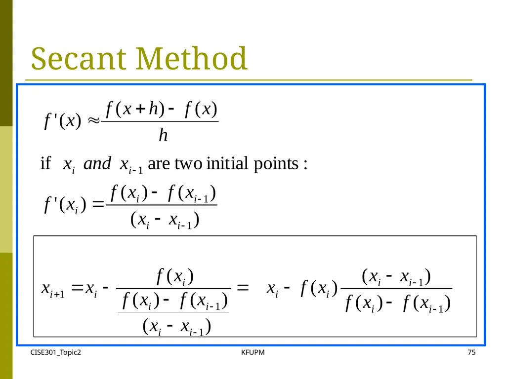
slide75. CISE301_Topic2 KFUPM 75 Secant Method<br>
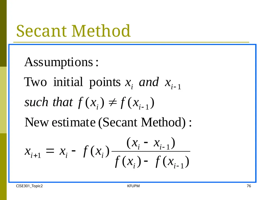
slide76. CISE301_Topic2 KFUPM 76 Secant Method<br>
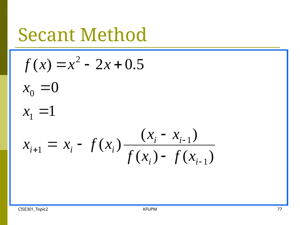
slide77. CISE301_Topic2 KFUPM 77 Secant Method<br>
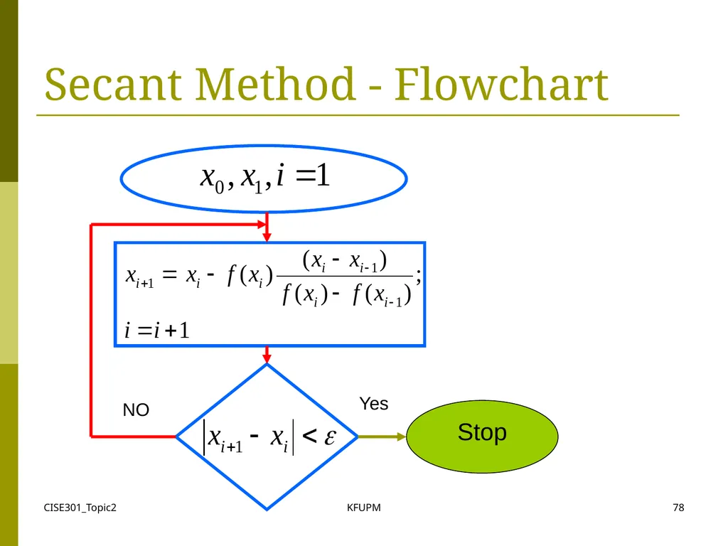
slide78. CISE301_Topic2 KFUPM 78 Secant Method - Flowchart Stop NO Yes<br>
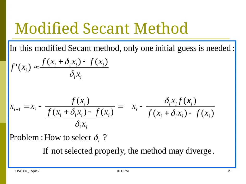
slide79. CISE301_Topic2 KFUPM 79 Modified Secant Method<br>
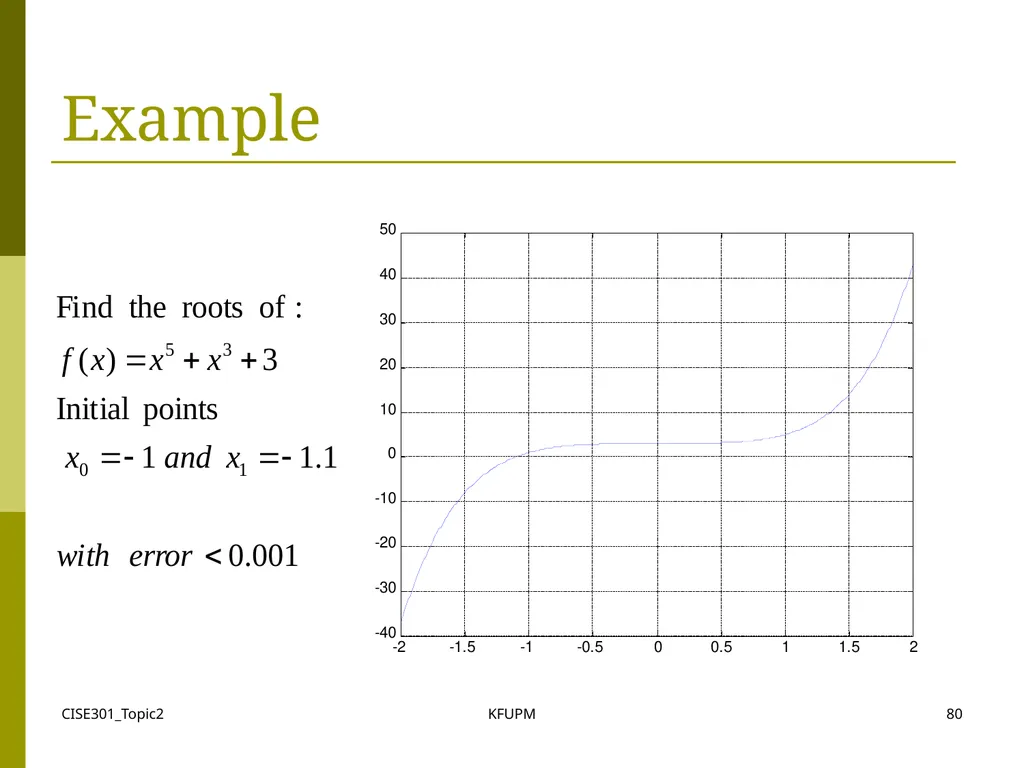
slide80. CISE301_Topic2 KFUPM 80 Example<br>
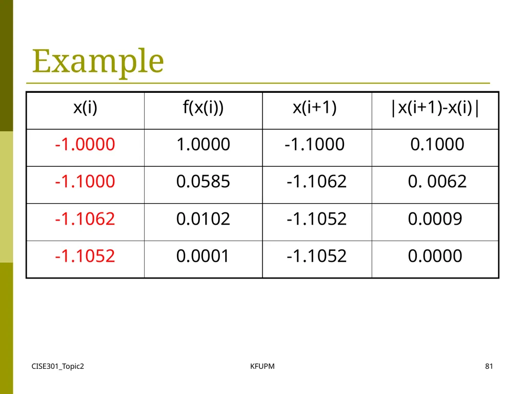
slide81. CISE301_Topic2 KFUPM 81 Example<br>
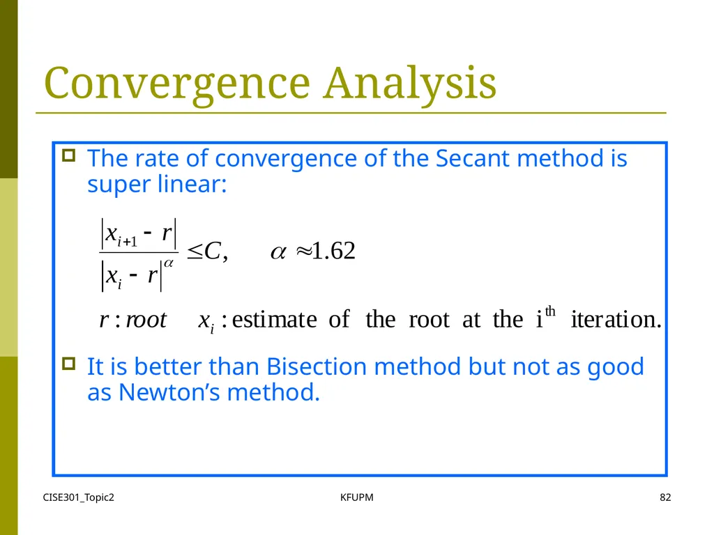
slide82. CISE301_Topic2 KFUPM 82 Convergence Analysis The rate of convergence of the Secant method is super linear:

It is better than Bisection method but not as good as Newton’s method.<br>
slide83. CISE301_Topic2 KFUPM 83 Lectures 11 Comparison of RootFinding Methods Advantages/disadvantages
Examples<br>
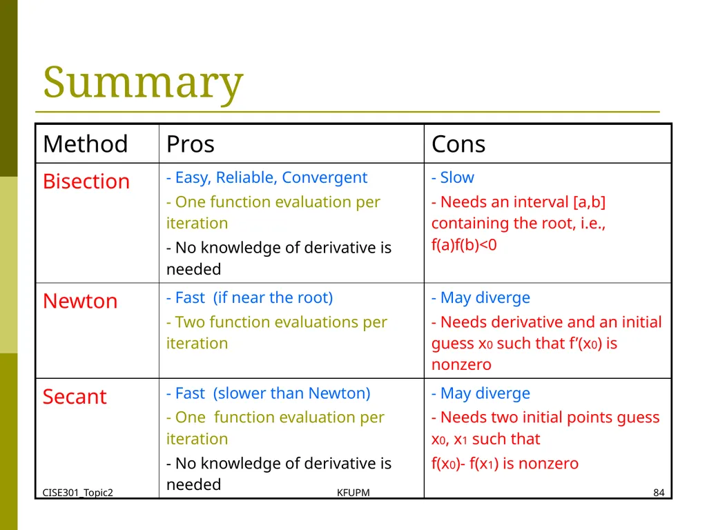
slide84. CISE301_Topic2 KFUPM 84 Summary<br>
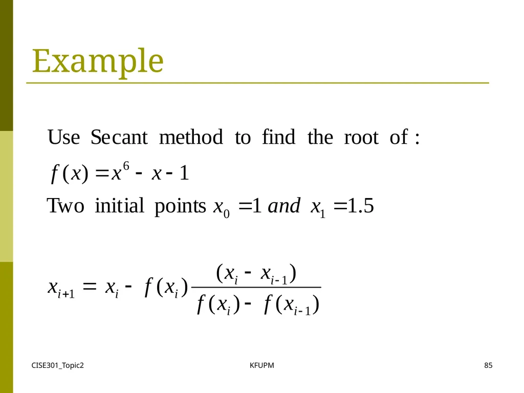
slide85. CISE301_Topic2 KFUPM 85 Example<br>
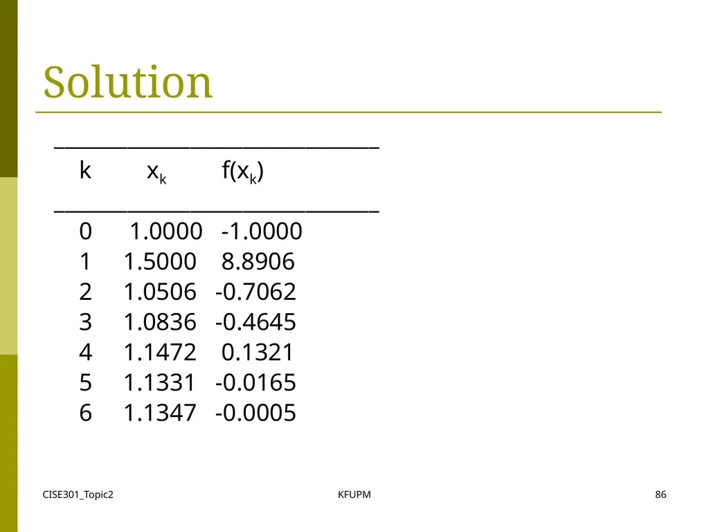
slide86. CISE301_Topic2 KFUPM 86 Solution _______________________________
k xk f(xk)
_______________________________
0 1.0000 -1.0000
1 1.5000 8.8906
2 1.0506 -0.7062
3 1.0836 -0.4645
4 1.1472 0.1321
5 1.1331 -0.0165
6 1.1347 -0.0005<br>
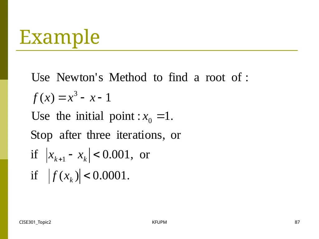
slide87. CISE301_Topic2 KFUPM 87 Example<br>
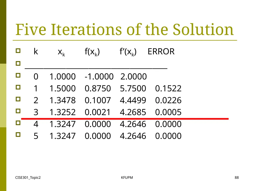
slide88. CISE301_Topic2 KFUPM 88 Five Iterations of the Solution k xk f(xk) f’(xk) ERROR
______________________________________
0 1.0000 -1.0000 2.0000
1 1.5000 0.8750 5.7500 0.1522
2 1.3478 0.1007 4.4499 0.0226
3 1.3252 0.0021 4.2685 0.0005
4 1.3247 0.0000 4.2646 0.0000
5 1.3247 0.0000 4.2646 0.0000<br>
slide89. CISE301_Topic2 KFUPM 89 Example<br>
slide90. CISE301_Topic2 KFUPM 90 Example<br>
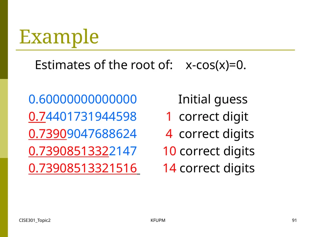
slide91. CISE301_Topic2 KFUPM 91 Example Estimates of the root of: x-cos(x)=0.

0.60000000000000 Initial guess
0.74401731944598 1 correct digit
0.73909047688624 4 correct digits
0.73908513322147 10 correct digits
0.73908513321516 14 correct digits<br>
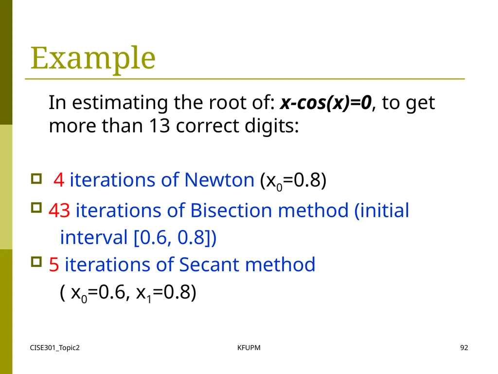
slide92. CISE301_Topic2 KFUPM 92 Example In estimating the root of: x-cos(x)=0, to get more than 13 correct digits:

4 iterations of Newton (x0=0.8)
43 iterations of Bisection method (initial
interval [0.6, 0.8])
5 iterations of Secant method
( x0=0.6, x1=0.8)<br>