
Data-Informed Environmental Conversion Updating
Description: Data-Informed Environmental Conversion Updating MIL-HDBK-217 and -338 with 50 years of field data Prepared for RAMS Training Summit XIV November 1-2, 2022 Huntsville, AL, US By Gwyer Sinclair (NASA) Describes a set of conditions in which a
Related Topics
Download Presentation
"Data-Informed Environmental Conversion Updating" is the property of its rightful owner. Permission is granted to download and print the materials on this website for personal, non-commercial use only, and to display it on your personal computer provided you do not modify the materials and that you retain all copyright notices contained in the materials. By downloading content from our website, you accept the terms of this agreement.
Presentation Transcript
slide1. Data-Informed Environmental Conversion
Updating MIL-HDBK-217 and -338 with 50+ years of field data Prepared for RAMS Training Summit XIV
November 1-2, 2022
Huntsville, AL, US
By Gwyer Sinclair (NASA)<br>
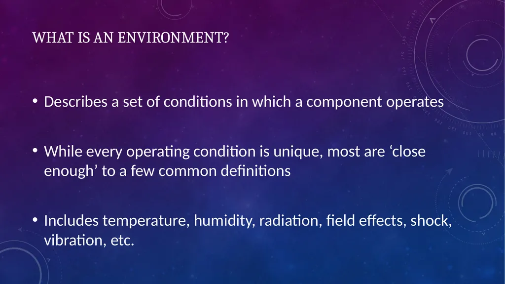
slide2. Describes a set of conditions in which a component operates
While every operating condition is unique, most are ‘close enough’ to a few common definitions
Includes temperature, humidity, radiation, field effects, shock, vibration, etc. What is an environment?<br>
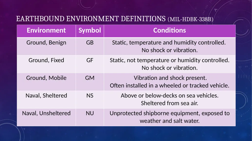
slide3. Earthbound Environment Definitions (MIL-HDBK-338B)<br>
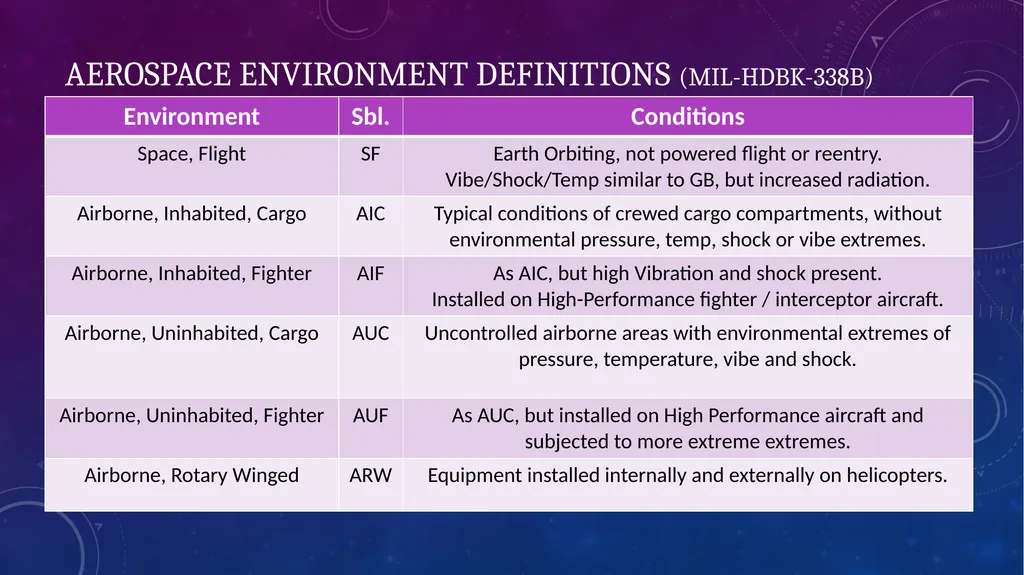
slide4. Aerospace Environment Definitions (MIL-HDBK-338B)<br>
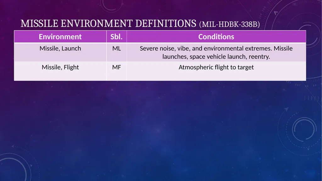
slide5. Missile Environment Definitions (MIL-HDBK-338B)<br>
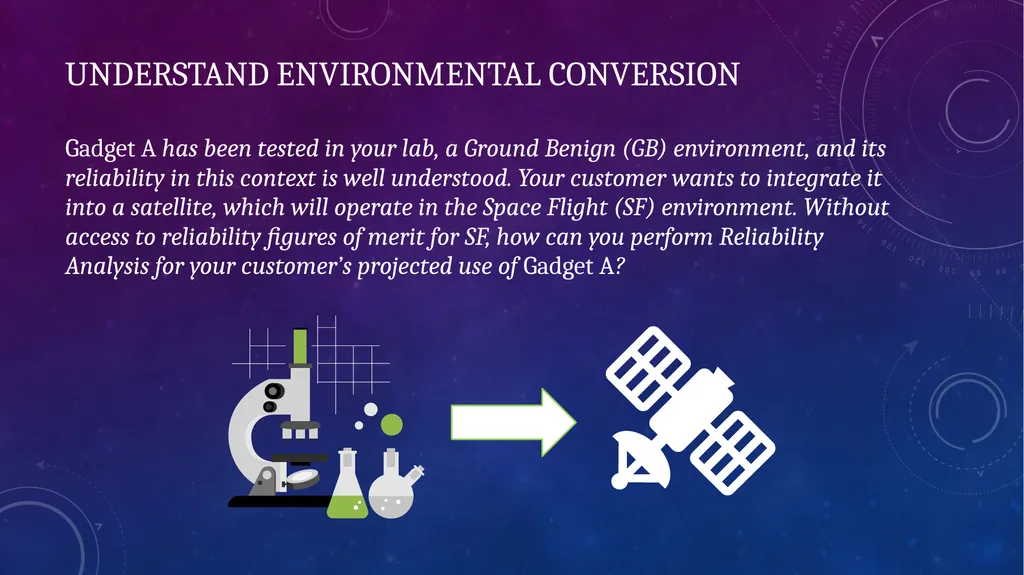
slide6. Understand environmental Conversion Gadget A has been tested in your lab, a Ground Benign (GB) environment, and its reliability in this context is well understood. Your customer wants to integrate it into a satellite, which will operate in the Space Flight (SF) environment. Without access to reliability figures of merit for SF, how can you perform Reliability Analysis for your customer’s projected use of Gadget A?<br>
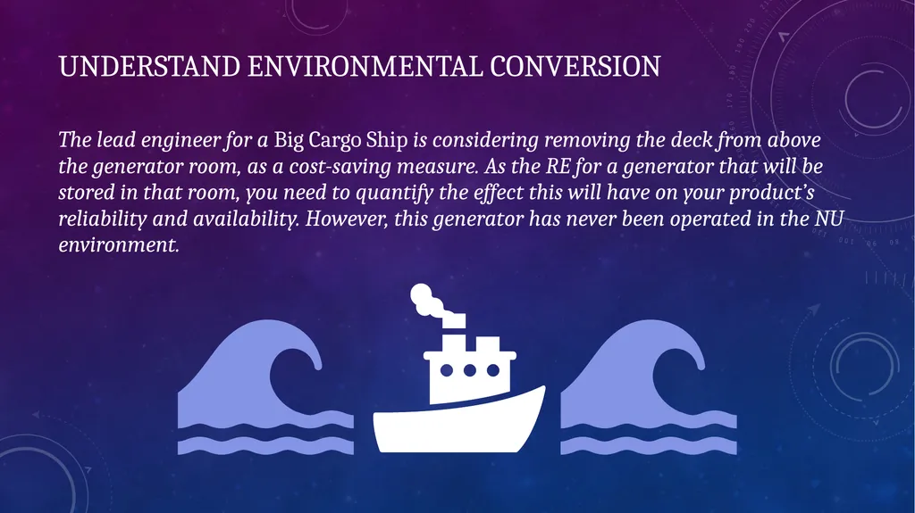
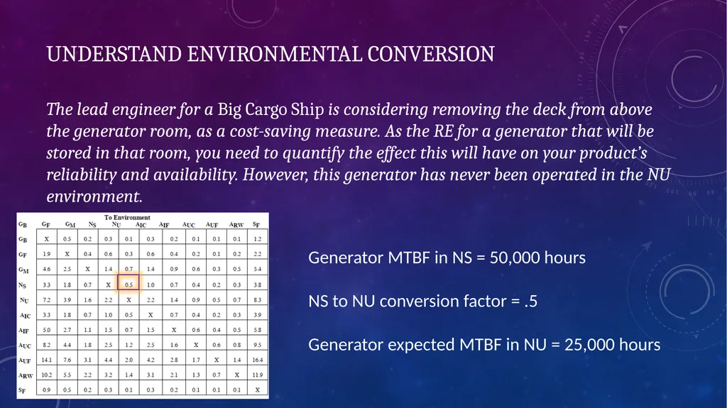
slide7. Understand environmental Conversion The lead engineer for a Big Cargo Ship is considering removing the deck from above the generator room, as a cost-saving measure. As the RE for a generator that will be stored in that room, you need to quantify the effect this will have on your product’s reliability and availability. However, this generator has never been operated in the NU environment.<br>
slide8. Understand environmental Conversion These situations can be modeled with Systems Reliability Engineering tools. Originally described in MIL-HDBK-217 and superseded by MIL-HDBK-338, techniques exist for converting between a known condition (quality, temperature, or environment) to an undemonstrated condition.
This is made possible by extensive study of the changes arising in well-studied parts when subjected to different conditions.<br>
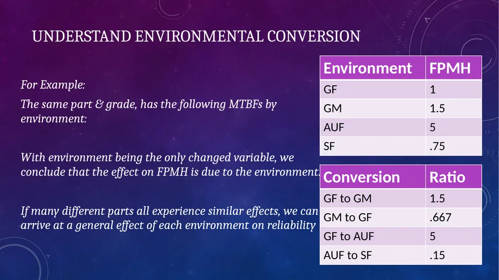
slide9. Understand environmental Conversion For Example:
The same part & grade, has the following MTBFs by environment:
With environment being the only changed variable, we conclude that the effect on FPMH is due to the environment.
If many different parts all experience similar effects, we can arrive at a general effect of each environment on reliability<br>
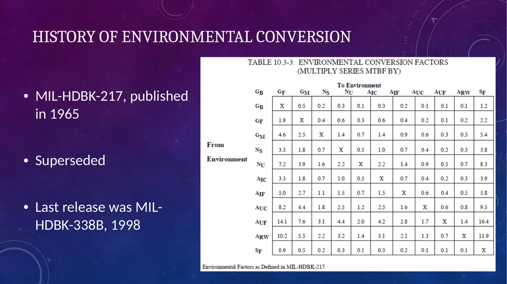
slide10. History of environmental Conversion MIL-HDBK-217, published in 1965
Superseded
Last release was MIL-HDBK-338B, 1998<br>
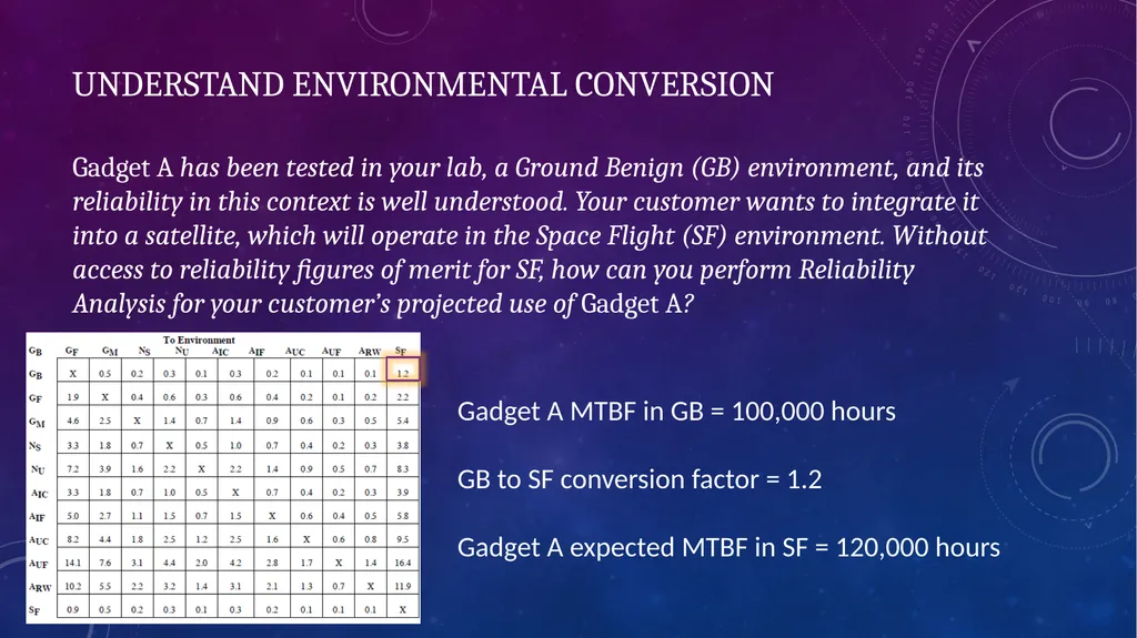
slide11. Understand environmental Conversion Gadget A has been tested in your lab, a Ground Benign (GB) environment, and its reliability in this context is well understood. Your customer wants to integrate it into a satellite, which will operate in the Space Flight (SF) environment. Without access to reliability figures of merit for SF, how can you perform Reliability Analysis for your customer’s projected use of Gadget A? Gadget A MTBF in GB = 100,000 hours
GB to SF conversion factor = 1.2
Gadget A expected MTBF in SF = 120,000 hours<br>
slide12. Understand environmental Conversion The lead engineer for a Big Cargo Ship is considering removing the deck from above the generator room, as a cost-saving measure. As the RE for a generator that will be stored in that room, you need to quantify the effect this will have on your product’s reliability and availability. However, this generator has never been operated in the NU environment. Generator MTBF in NS = 50,000 hours
NS to NU conversion factor = .5
Generator expected MTBF in NU = 25,000 hours<br>
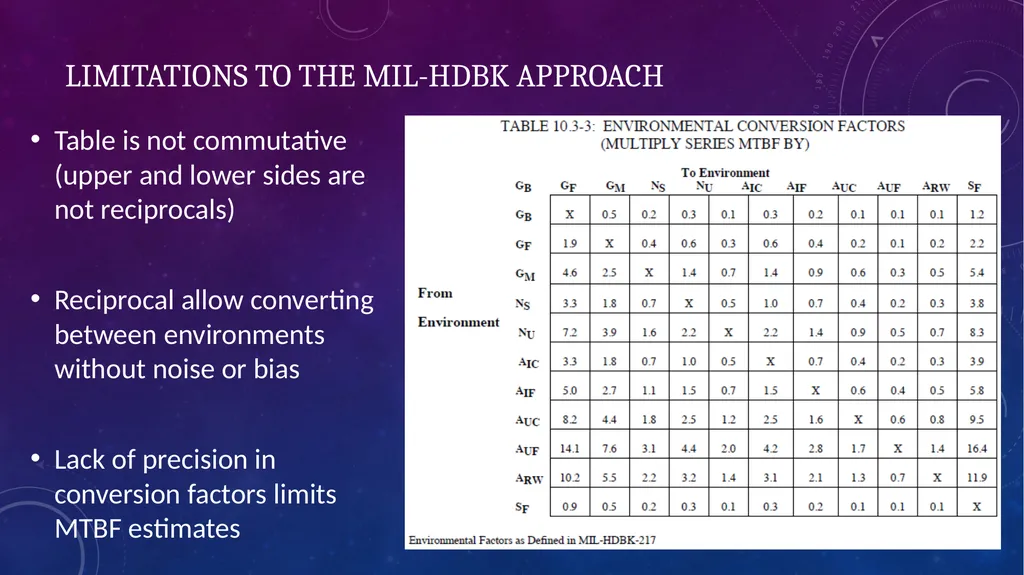
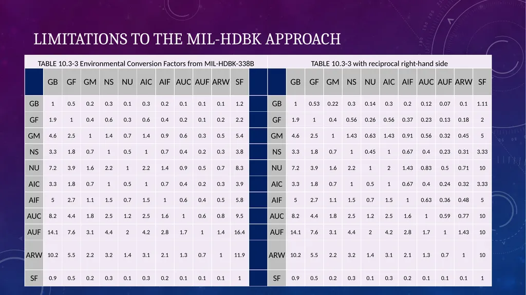
slide13. Limitations to the MIL-HDBK Approach Table is not commutative (upper and lower sides are not reciprocals)
Reciprocal allow converting between environments without noise or bias
Lack of precision in conversion factors limits MTBF estimates<br>
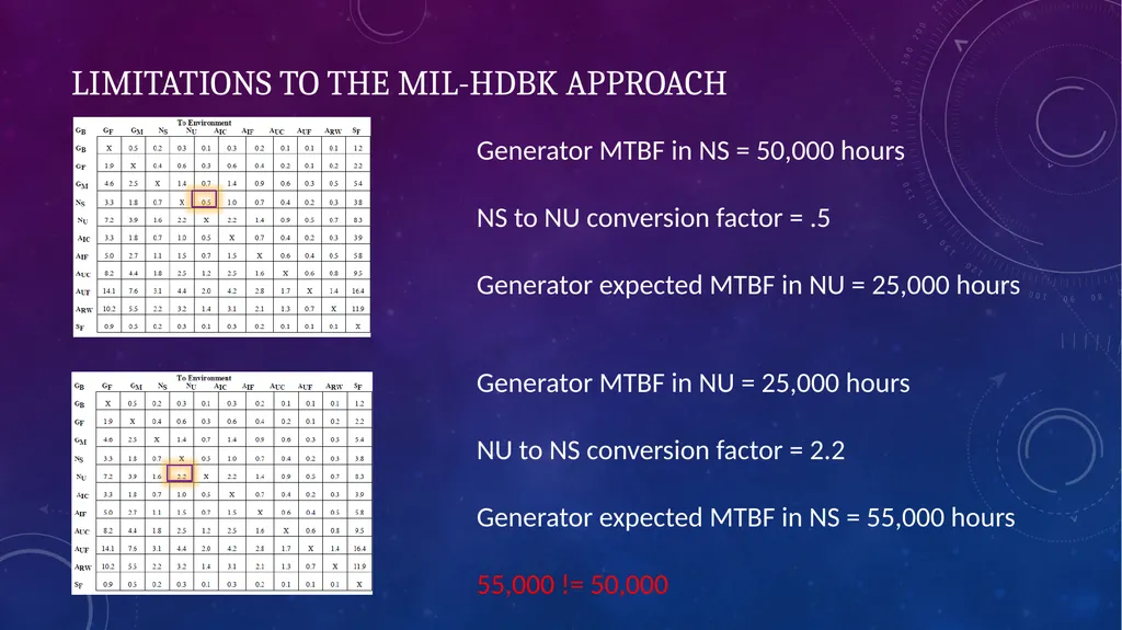
slide14. Limitations to the MIL-HDBK Approach Generator MTBF in NS = 50,000 hours
NS to NU conversion factor = .5
Generator expected MTBF in NU = 25,000 hours Generator MTBF in NU = 25,000 hours
NU to NS conversion factor = 2.2
Generator expected MTBF in NS = 55,000 hours
55,000 != 50,000<br>
slide15. Limitations to the MIL-HDBK Approach<br>
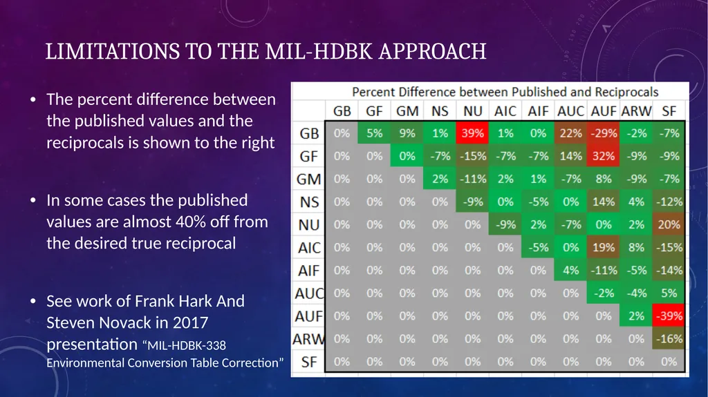
slide16. Limitations to the MIL-HDBK Approach The percent difference between the published values and the reciprocals is shown to the right
In some cases the published values are almost 40% off from the desired true reciprocal
See work of Frank Hark And Steven Novack in 2017 presentation “MIL-HDBK-338 Environmental Conversion Table Correction”<br>
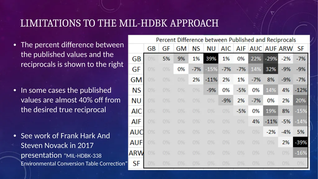
slide17. Limitations to the MIL-HDBK Approach The percent difference between the published values and the reciprocals is shown to the right
In some cases the published values are almost 40% off from the desired true reciprocal
See work of Frank Hark And Steven Novack in 2017 presentation “MIL-HDBK-338 Environmental Conversion Table Correction”<br>
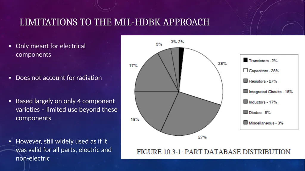
slide18. Limitations to the MIL-HDBK Approach Only meant for electrical components
Does not account for radiation
Based largely on only 4 component varieties – limited use beyond these components
However, still widely used as if it was valid for all parts, electric and non-electric<br>
slide19. Solution – update the MIL-HDBK Approach Now have 50+ years of field data beyond what was available to MIL-HDBK-217 authors in 1965
Update the Environmental Conversions Table for Electrical-Only components
Build a new table for All Parts, electric and mechanical
Questions on applications and history of Environmental conversion?<br>
slide20. A look at The Data What field data is available?
Why should we trust this data?
How limited is the available data?<br>
slide21. What field data is available? Military specs and studies
Government database
Industry / Private database<br>
slide22. Why should we trust this data? Dependent on source
In general, tests performed over like lots and large sample time
In this meta-study, data cleaning including removing outliers can control for misreporting<br>
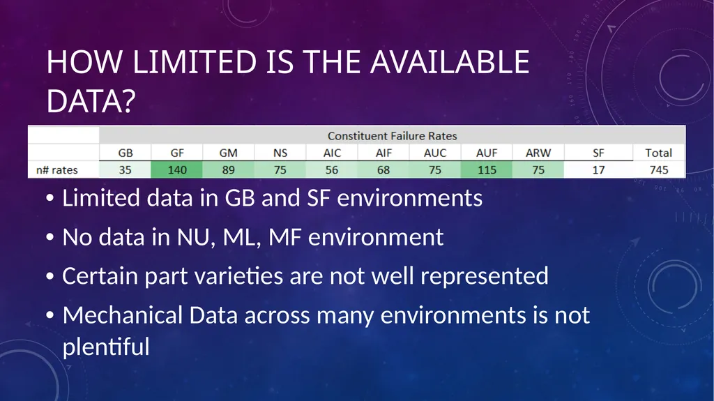
slide23. How limited is the available data? Limited data in GB and SF environments
No data in NU, ML, MF environment
Certain part varieties are not well represented
Mechanical Data across many environments is not plentiful<br>
slide24. A look at the methodology Examine notional data (cannot share proprietary data)
Criteria for including data in this analysis
Demonstrate the method to build a new table<br>
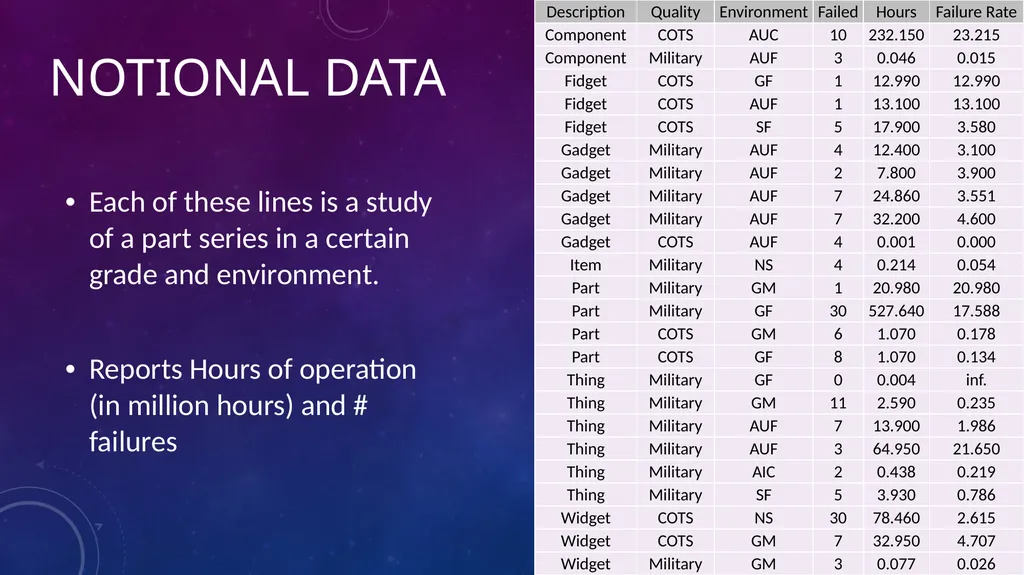
slide25. notional data Each of these lines is a study of a part series in a certain grade and environment.
Reports Hours of operation (in million hours) and # failures<br>
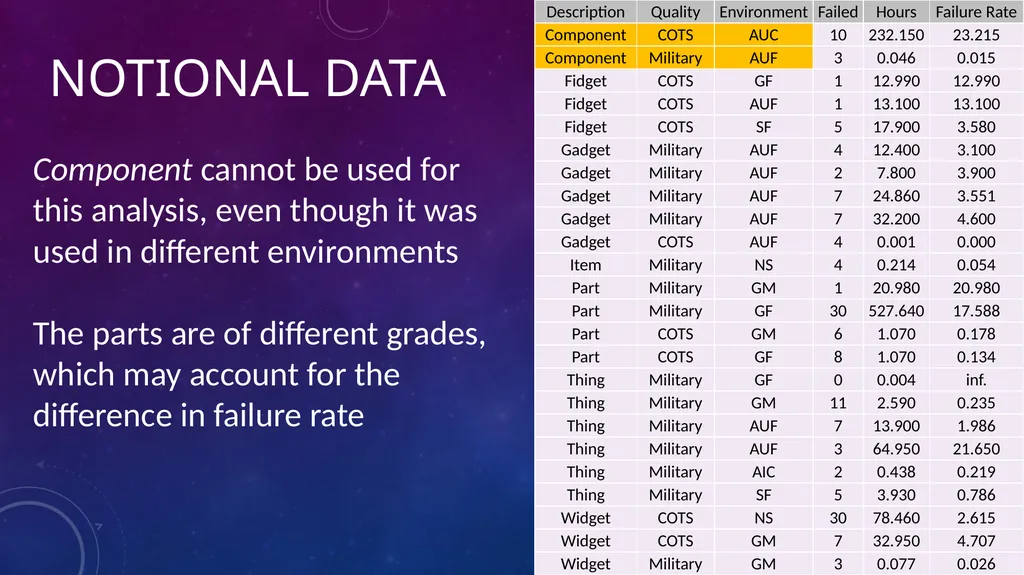
slide26. notional data Component cannot be used for this analysis, even though it was used in different environments
The parts are of different grades, which may account for the difference in failure rate<br>
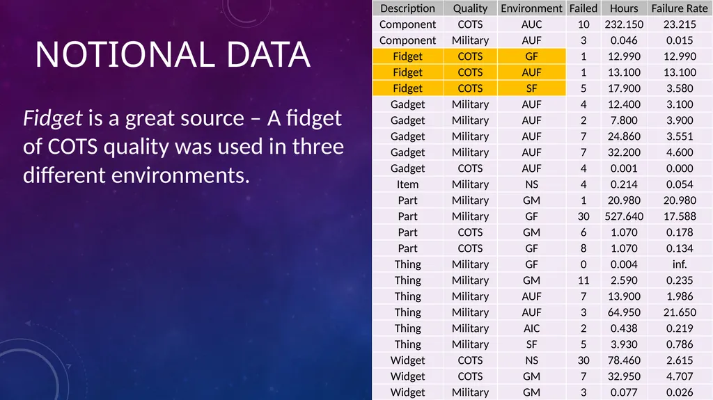
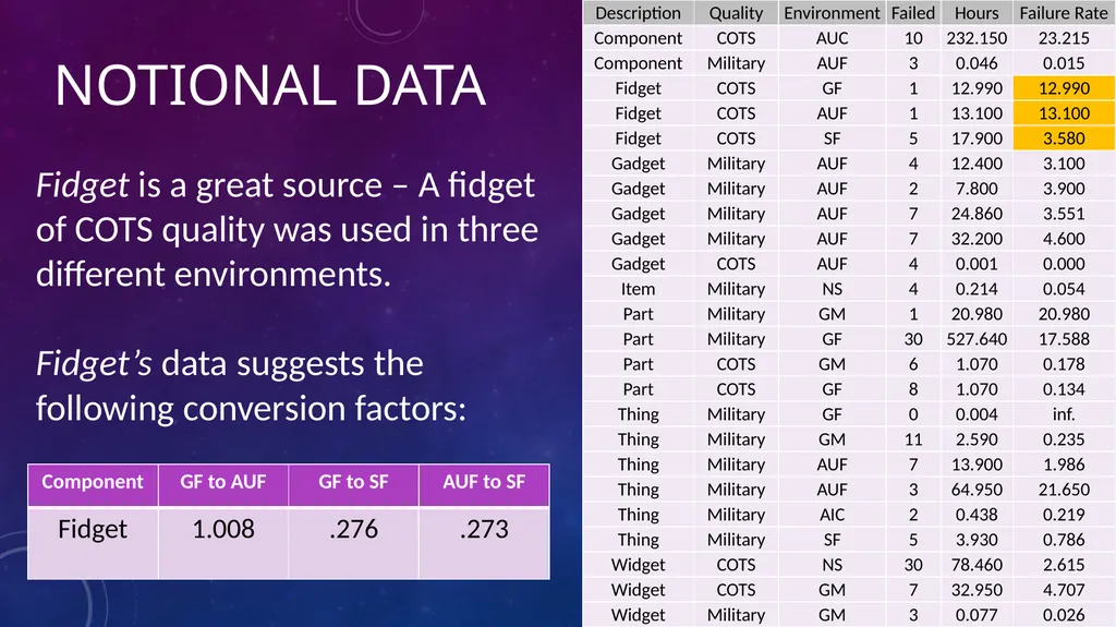
slide27. notional data Fidget is a great source – A fidget of COTS quality was used in three different environments.<br>
slide28. notional data Fidget is a great source – A fidget of COTS quality was used in three different environments.
Fidget’s data suggests the following conversion factors:<br>
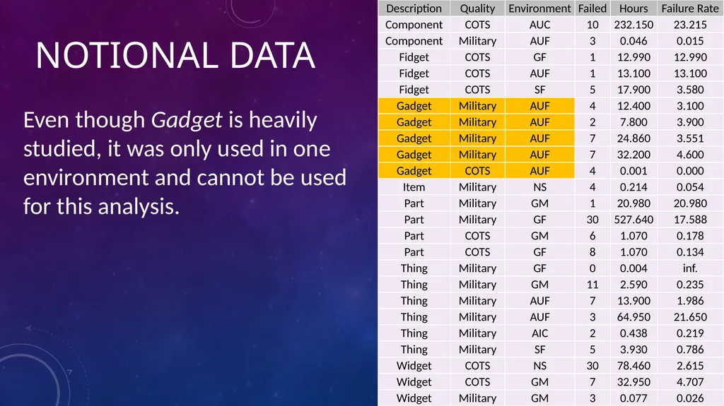
slide29. notional data Even though Gadget is heavily studied, it was only used in one environment and cannot be used for this analysis.<br>
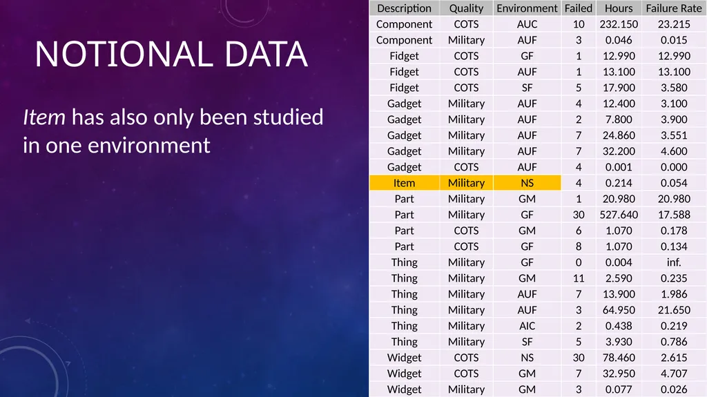
slide30. notional data Item has also only been studied in one environment<br>
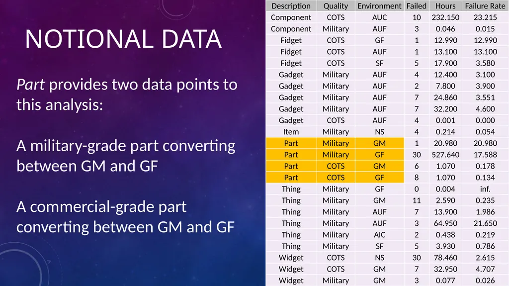
slide31. notional data Part provides two data points to this analysis:
A military-grade part converting between GM and GF
A commercial-grade part converting between GM and GF<br>
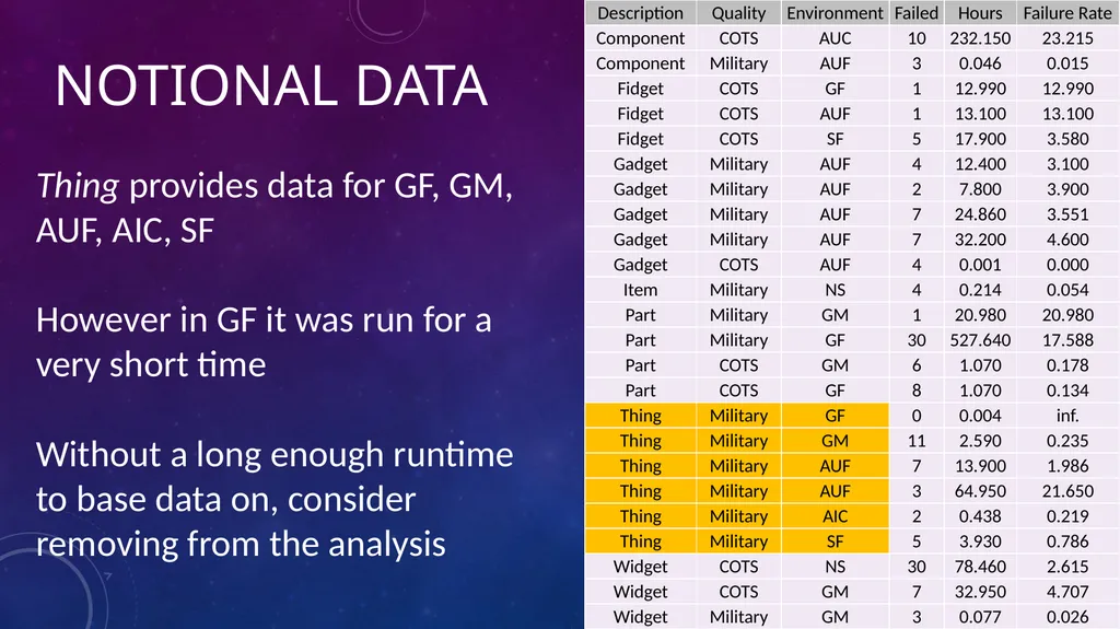
slide32. notional data Thing provides data for GF, GM, AUF, AIC, SF
However in GF it was run for a very short time
Without a long enough runtime to base data on, consider removing from the analysis<br>
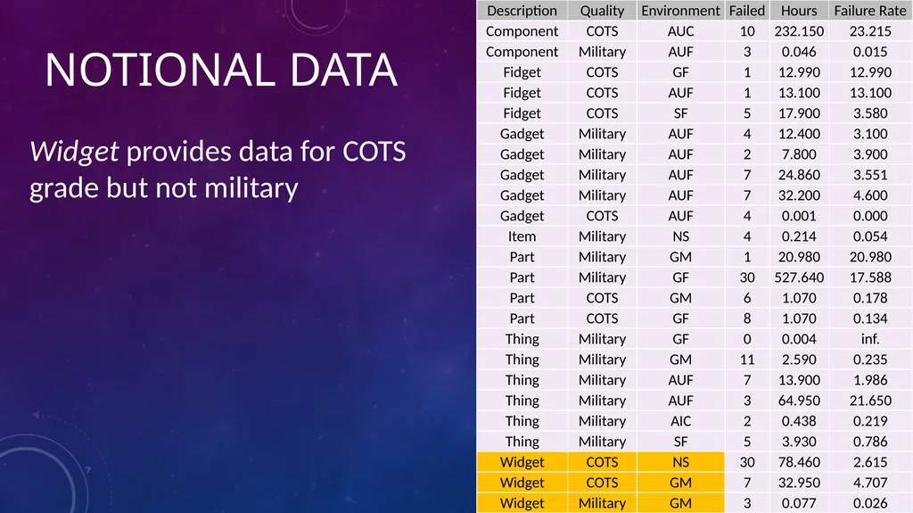
slide33. notional data Widget provides data for COTS grade but not military<br>
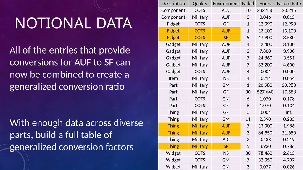
slide34. notional data All of the entries that provide conversions for AUF to SF can now be combined to create a generalized conversion ratio
With enough data across diverse parts, build a full table of generalized conversion factors<br>
slide35. Analysis outputs Examine constituent real world data
Review statistics and limitations
Present results<br>
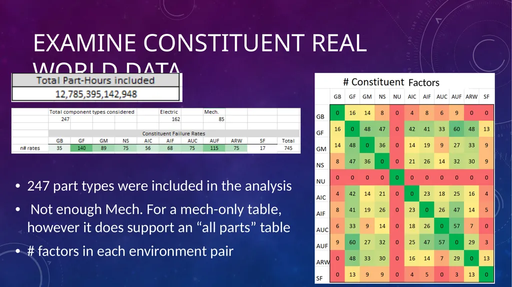
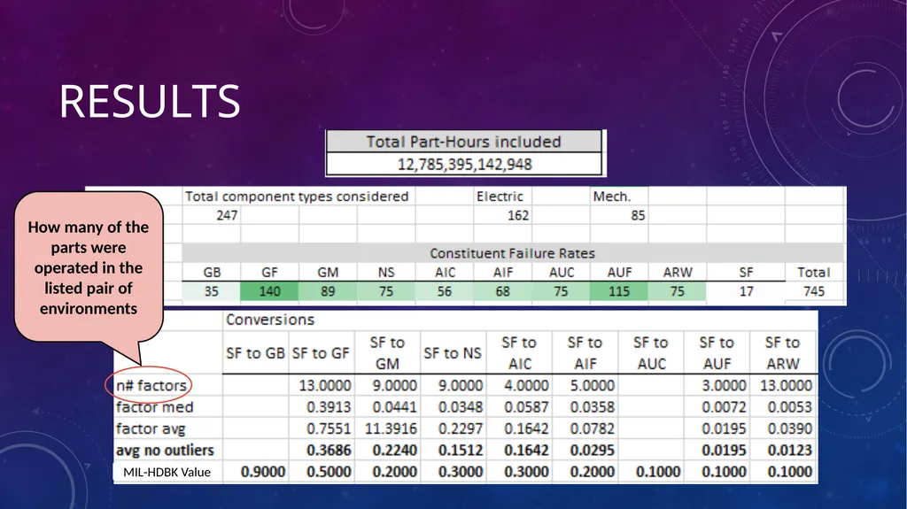
slide36. Examine constituent real world data 247 part types were included in the analysis
Not enough Mech. For a mech-only table, however it does support an “all parts” table
# factors in each environment pair Factors<br>
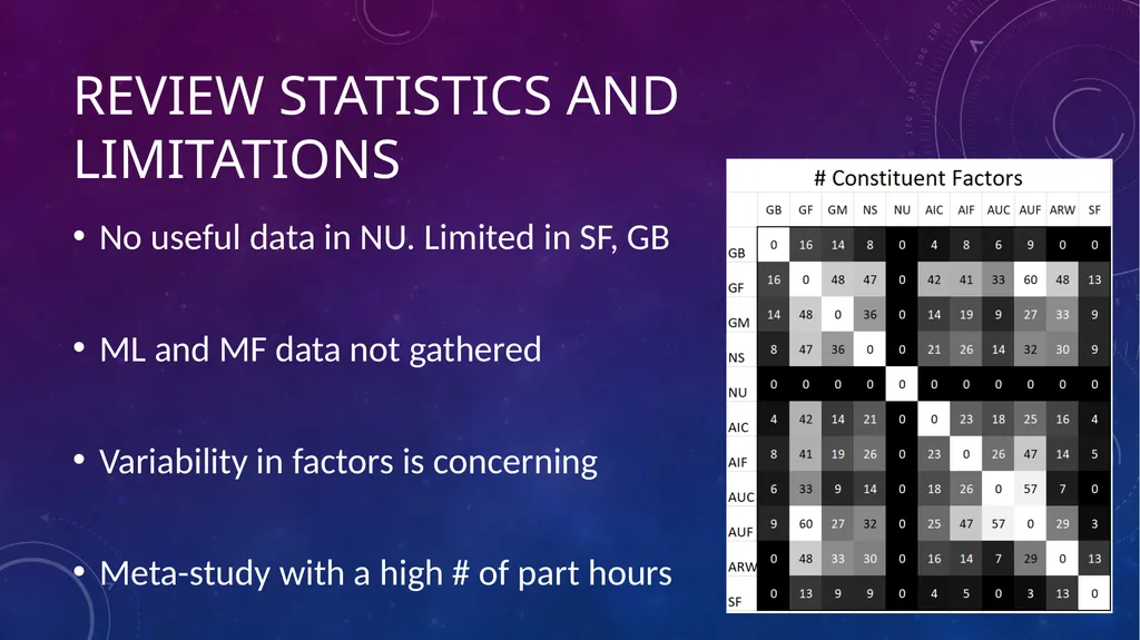
slide37. Review statistics and limitations No useful data in NU. Limited in SF, GB
ML and MF data not gathered
Variability in factors is concerning
Meta-study with a high # of part hours<br>
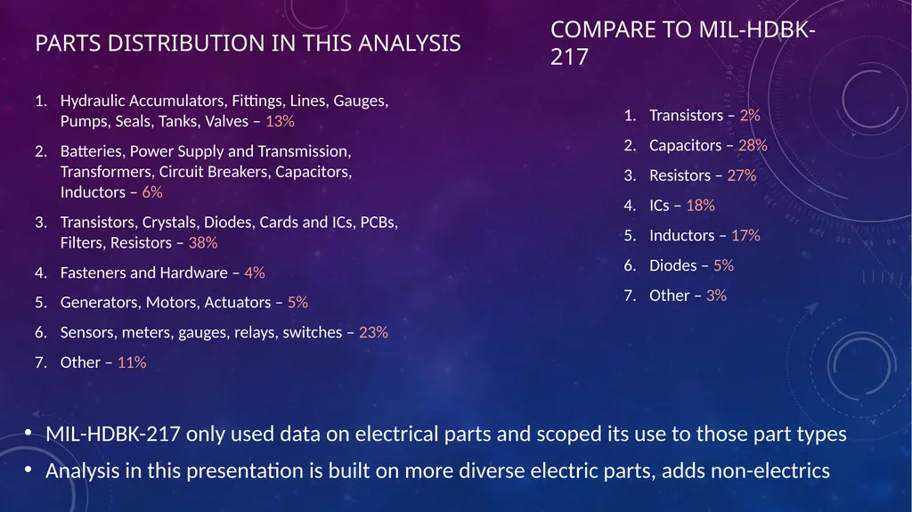
slide38. Hydraulic Accumulators, Fittings, Lines, Gauges, Pumps, Seals, Tanks, Valves – 13%
Batteries, Power Supply and Transmission, Transformers, Circuit Breakers, Capacitors, Inductors – 6%
Transistors, Crystals, Diodes, Cards and ICs, PCBs, Filters, Resistors – 38%
Fasteners and Hardware – 4%
Generators, Motors, Actuators – 5%
Sensors, meters, gauges, relays, switches – 23%
Other – 11% Compare to MIL-HDBK-217 Parts Distribution In this analysis MIL-HDBK-217 only used data on electrical parts and scoped its use to those part types
Analysis in this presentation is built on more diverse electric parts, adds non-electrics Transistors – 2%
Capacitors – 28%
Resistors – 27%
ICs – 18%
Inductors – 17%
Diodes – 5%
Other – 3%<br>
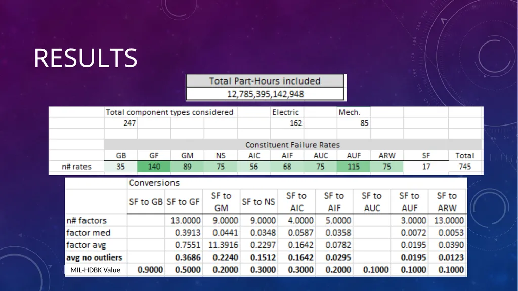
slide39. Results MIL-HDBK Value<br>
slide40. Results How many of the parts were operated in the listed pair of environments MIL-HDBK Value<br>
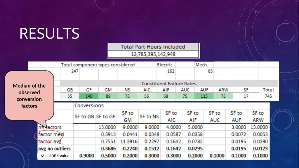
slide41. Results Median of the observed conversion factors MIL-HDBK Value<br>
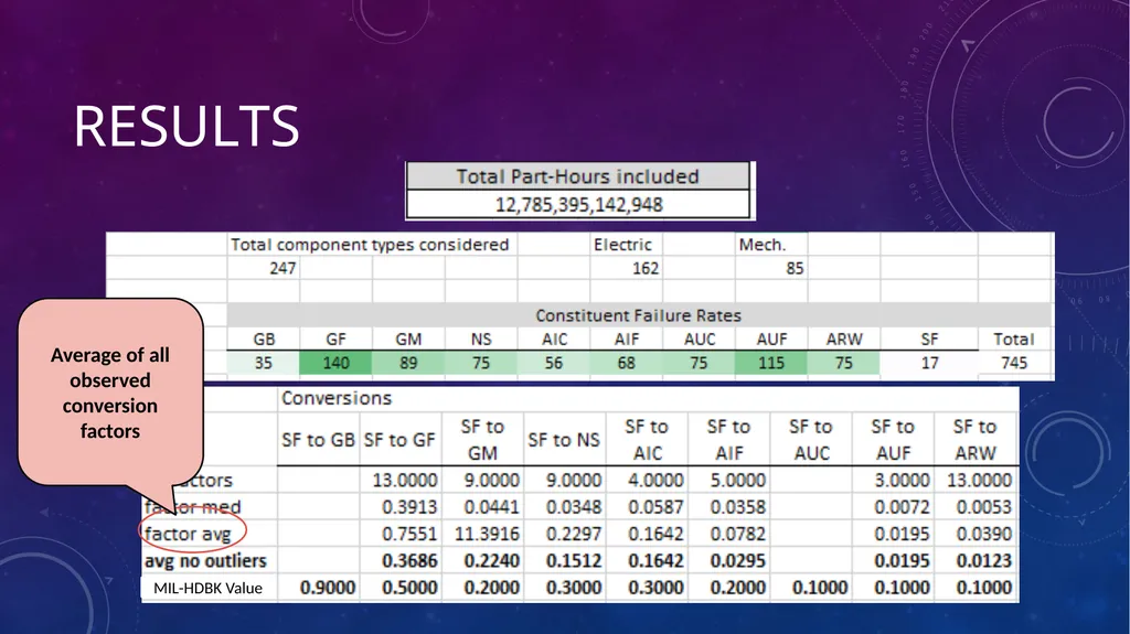
slide42. Results Average of all observed conversion factors MIL-HDBK Value<br>
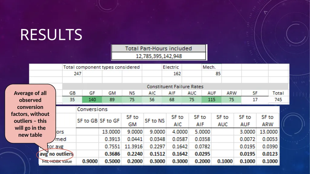
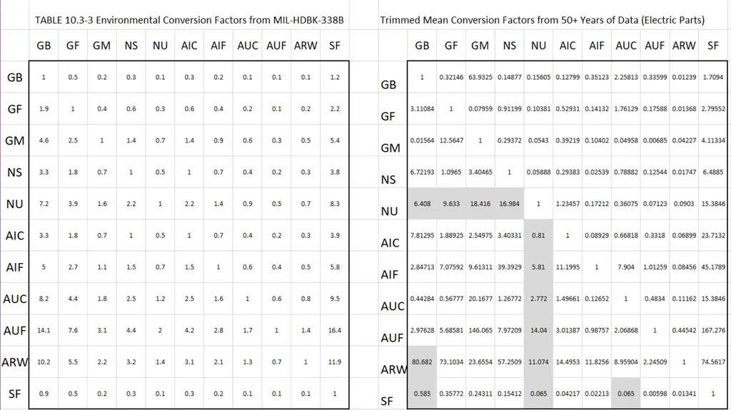
slide43. Results Average of all observed conversion factors, without outliers – this will go in the new table MIL-HDBK Value<br>
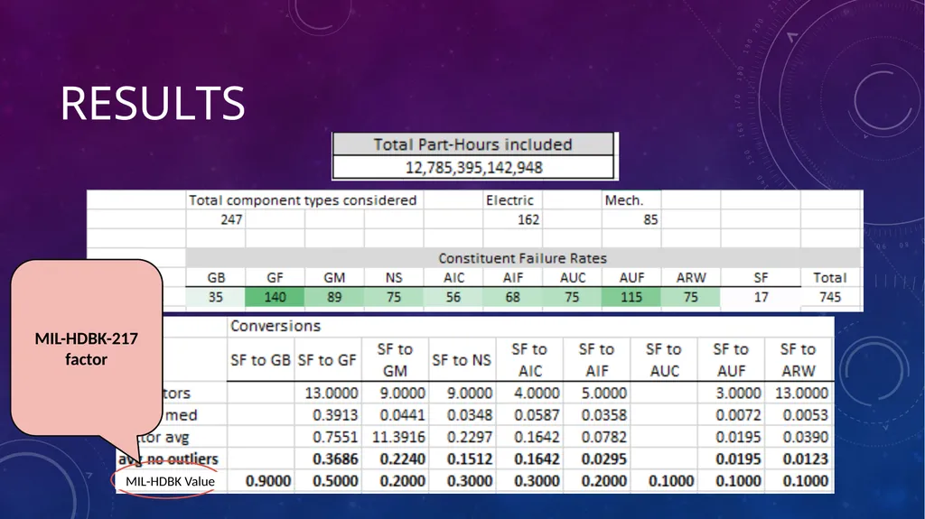
slide44. Results MIL-HDBK-217 factor MIL-HDBK Value<br>
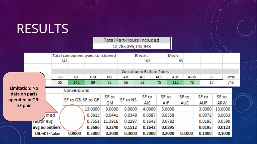
slide45. Results Limitation: No data on parts operated in GB-SF pair MIL-HDBK Value<br>
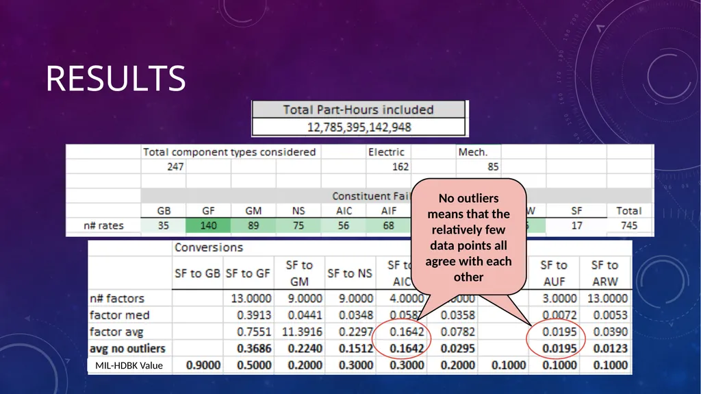
slide46. Results No outliers means that the relatively few data points all agree with each other MIL-HDBK Value<br>
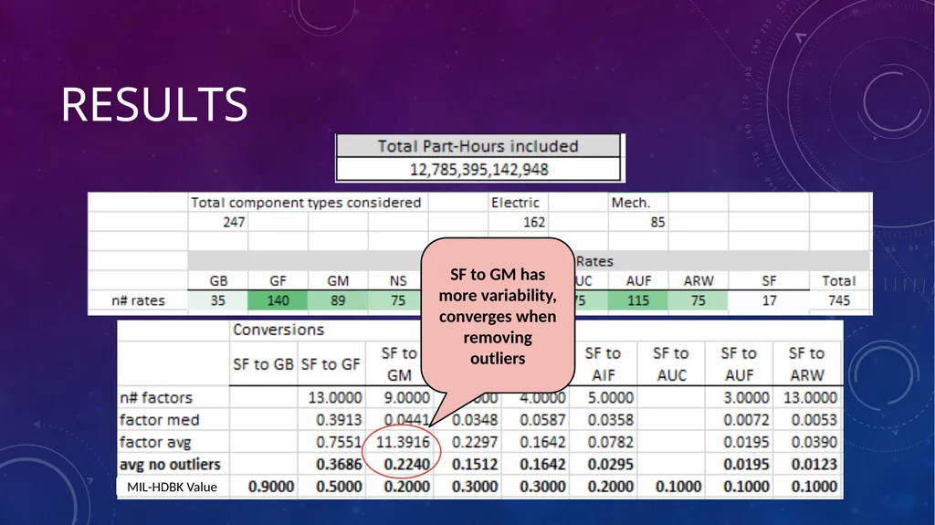
slide47. Results SF to GM has more variability, converges when removing outliers MIL-HDBK Value<br>
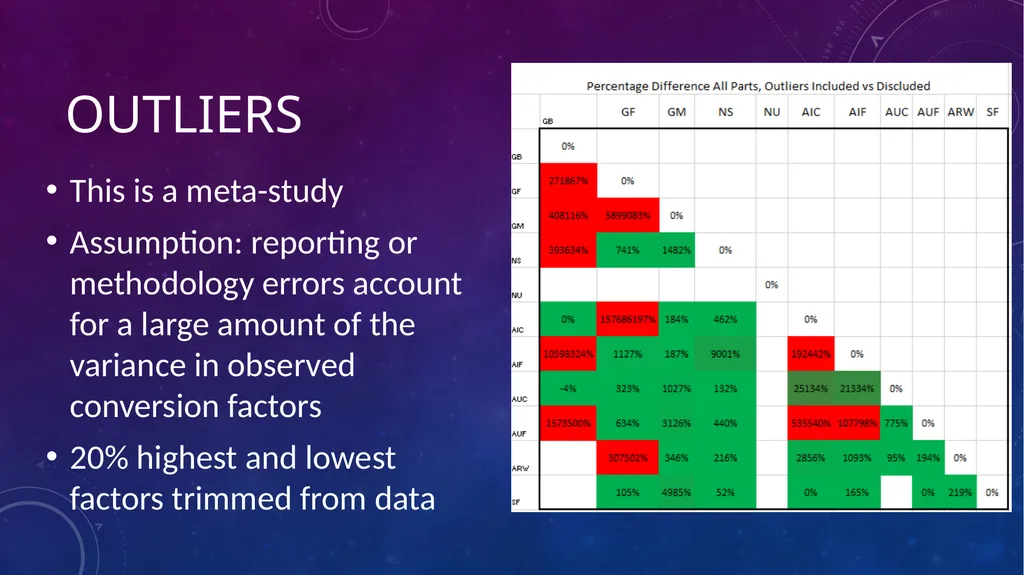
slide48. outliers This is a meta-study
Assumption: reporting or methodology errors account for a large amount of the variance in observed conversion factors
20% highest and lowest factors trimmed from data<br>
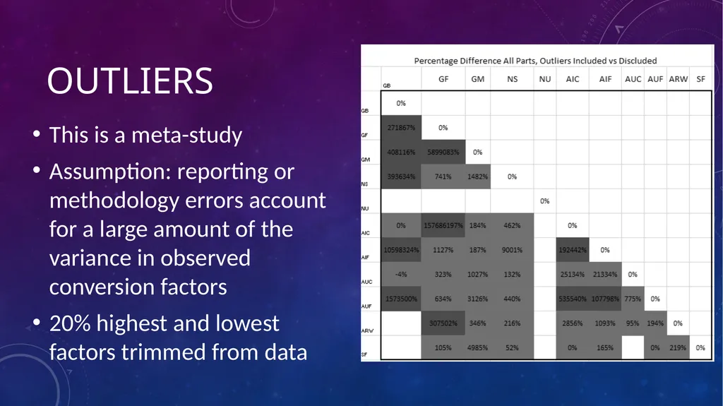
slide49. outliers This is a meta-study
Assumption: reporting or methodology errors account for a large amount of the variance in observed conversion factors
20% highest and lowest factors trimmed from data<br>
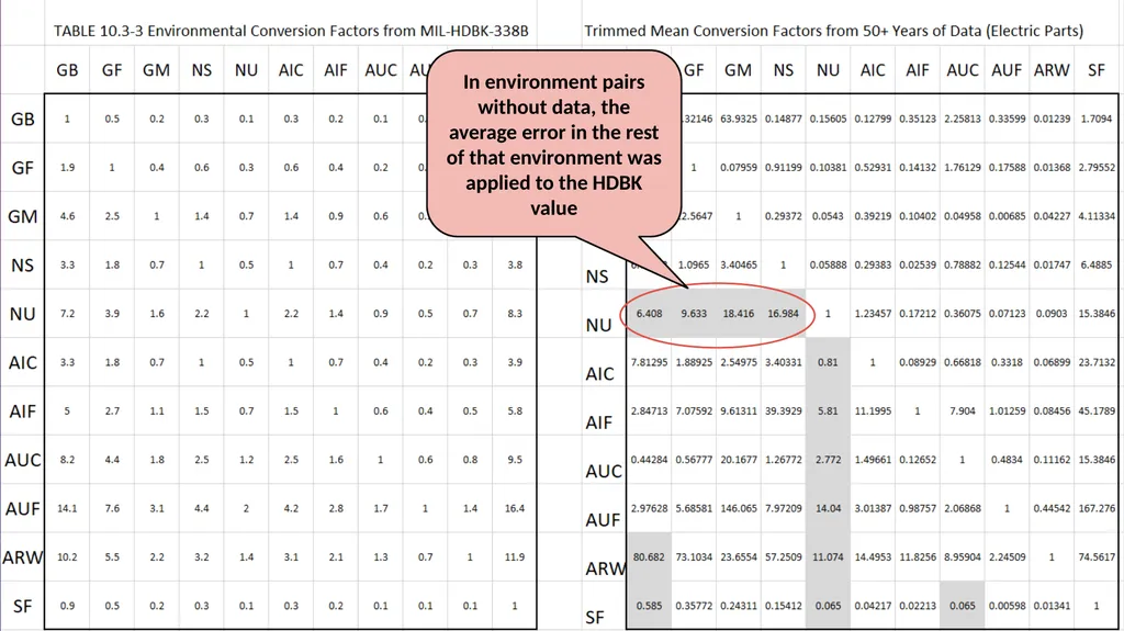
slide51. In environment pairs without data, the average error in the rest of that environment was applied to the HDBK value<br>
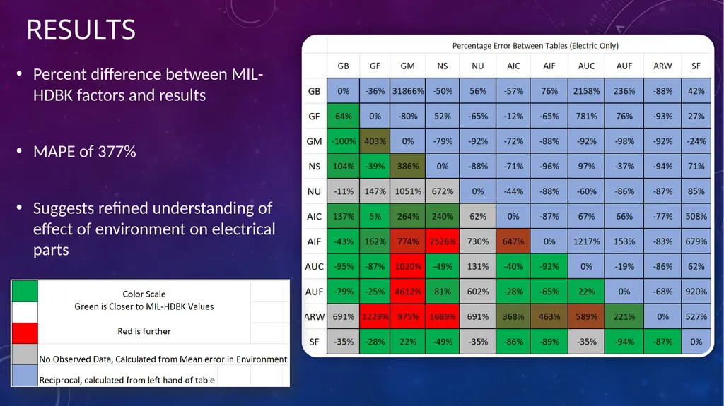
slide52. Results Percent difference between MIL-HDBK factors and results
MAPE of 377%
Suggests refined understanding of effect of environment on electrical parts<br>
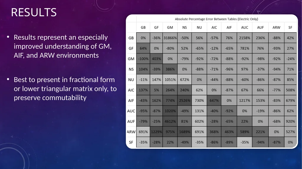
slide53. Results Results represent an especially improved understanding of GM, AIF, and ARW environments
Best to present in fractional form or lower triangular matrix only, to preserve commutability<br>
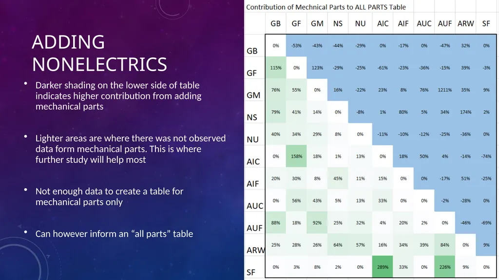
slide54. Adding nonelectrics Darker shading on the lower side of table indicates higher contribution from adding mechanical parts
Lighter areas are where there was not observed data form mechanical parts. This is where further study will help most
Not enough data to create a table for mechanical parts only
Can however inform an “all parts” table<br>
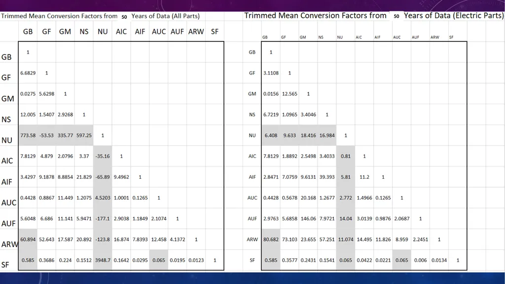
slide55. 50 50<br>
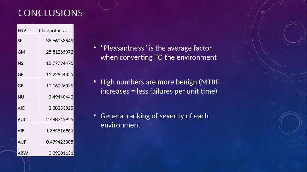
slide56. Conclusions “Pleasantness” is the average factor when converting TO the environment
High numbers are more benign (MTBF increases = less failures per unit time)
General ranking of severity of each environment<br>
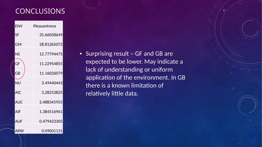
slide57. Conclusions Surprising result – GF and GB are expected to be lower. May indicate a lack of understanding or uniform application of the environment. In GB there is a known limitation of relatively little data.<br>
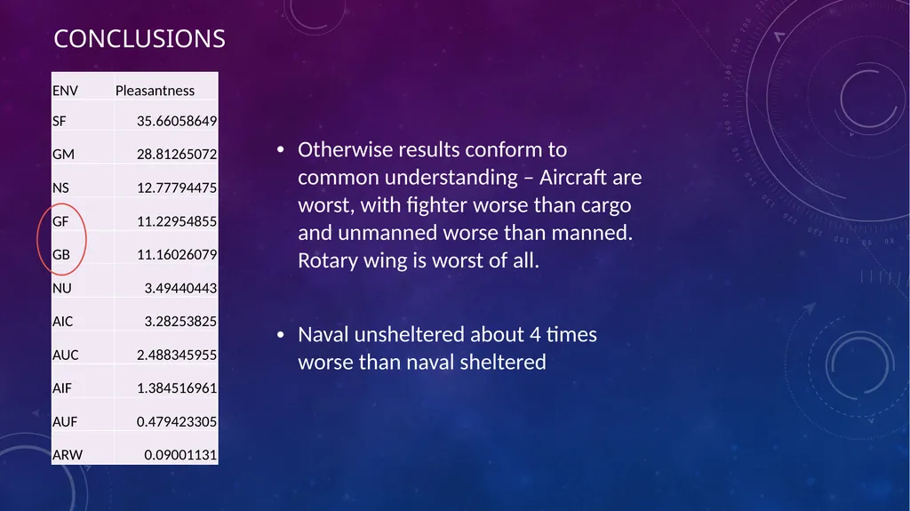
slide58. Conclusions Otherwise results conform to common understanding – Aircraft are worst, with fighter worse than cargo and unmanned worse than manned. Rotary wing is worst of all.
Naval unsheltered about 4 times worse than naval sheltered<br>
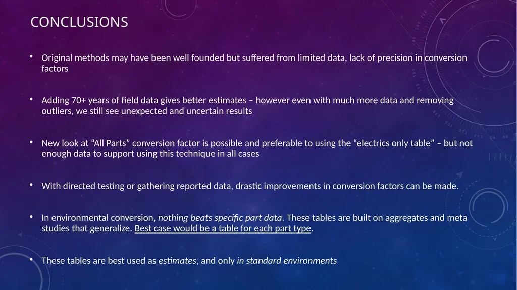
slide59. Conclusions Original methods may have been well founded but suffered from limited data, lack of precision in conversion factors
Adding 70+ years of field data gives better estimates – however even with much more data and removing outliers, we still see unexpected and uncertain results
New look at “All Parts” conversion factor is possible and preferable to using the “electrics only table” – but not enough data to support using this technique in all cases
With directed testing or gathering reported data, drastic improvements in conversion factors can be made.
In environmental conversion, nothing beats specific part data. These tables are built on aggregates and meta studies that generalize. Best case would be a table for each part type.
These tables are best used as estimates, and only in standard environments<br>
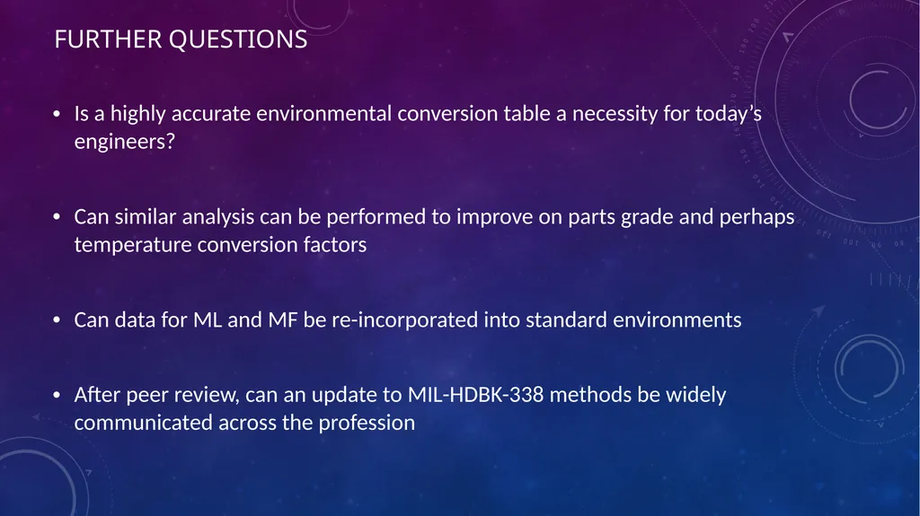
slide60. further questions Is a highly accurate environmental conversion table a necessity for today’s engineers?
Can similar analysis can be performed to improve on parts grade and perhaps temperature conversion factors
Can data for ML and MF be re-incorporated into standard environments
After peer review, can an update to MIL-HDBK-338 methods be widely communicated across the profession<br>
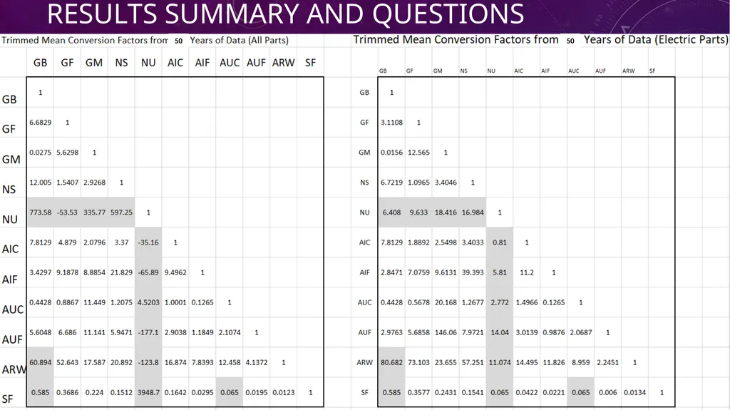
slide61. Results summary and questions 50 50<br>
slide62. References Frank Hark and Steven Novack, 2017 “MIL-HDBK-338 Environmental Conversion Table Correction”
MIL-HDBK-217 and -338B, DoD
Nonelectronic Parts Reliability Data Publication (NPRD-2016) – Quanterion Solutions Incorporated<br>
slide63. Backup – Grade Conversion Following the dissolution of a military-grade widget supplier, your project requires you to find a new source for the Particular Widget they had been producing. A candidate supplier, Cost Savers LLC, produces a Particular Widget at commercial-grade. How can you quantify the effect that this supplier substitution will have on the program’s overall reliability?<br>
November 1-2, 2022
Huntsville, AL, US
By Gwyer Sinclair (NASA)<br>
slide2. Describes a set of conditions in which a component operates
While every operating condition is unique, most are ‘close enough’ to a few common definitions
Includes temperature, humidity, radiation, field effects, shock, vibration, etc. What is an environment?<br>
slide3. Earthbound Environment Definitions (MIL-HDBK-338B)<br>
slide4. Aerospace Environment Definitions (MIL-HDBK-338B)<br>
slide5. Missile Environment Definitions (MIL-HDBK-338B)<br>
slide6. Understand environmental Conversion Gadget A has been tested in your lab, a Ground Benign (GB) environment, and its reliability in this context is well understood. Your customer wants to integrate it into a satellite, which will operate in the Space Flight (SF) environment. Without access to reliability figures of merit for SF, how can you perform Reliability Analysis for your customer’s projected use of Gadget A?<br>
slide7. Understand environmental Conversion The lead engineer for a Big Cargo Ship is considering removing the deck from above the generator room, as a cost-saving measure. As the RE for a generator that will be stored in that room, you need to quantify the effect this will have on your product’s reliability and availability. However, this generator has never been operated in the NU environment.<br>
slide8. Understand environmental Conversion These situations can be modeled with Systems Reliability Engineering tools. Originally described in MIL-HDBK-217 and superseded by MIL-HDBK-338, techniques exist for converting between a known condition (quality, temperature, or environment) to an undemonstrated condition.
This is made possible by extensive study of the changes arising in well-studied parts when subjected to different conditions.<br>
slide9. Understand environmental Conversion For Example:
The same part & grade, has the following MTBFs by environment:
With environment being the only changed variable, we conclude that the effect on FPMH is due to the environment.
If many different parts all experience similar effects, we can arrive at a general effect of each environment on reliability<br>
slide10. History of environmental Conversion MIL-HDBK-217, published in 1965
Superseded
Last release was MIL-HDBK-338B, 1998<br>
slide11. Understand environmental Conversion Gadget A has been tested in your lab, a Ground Benign (GB) environment, and its reliability in this context is well understood. Your customer wants to integrate it into a satellite, which will operate in the Space Flight (SF) environment. Without access to reliability figures of merit for SF, how can you perform Reliability Analysis for your customer’s projected use of Gadget A? Gadget A MTBF in GB = 100,000 hours
GB to SF conversion factor = 1.2
Gadget A expected MTBF in SF = 120,000 hours<br>
slide12. Understand environmental Conversion The lead engineer for a Big Cargo Ship is considering removing the deck from above the generator room, as a cost-saving measure. As the RE for a generator that will be stored in that room, you need to quantify the effect this will have on your product’s reliability and availability. However, this generator has never been operated in the NU environment. Generator MTBF in NS = 50,000 hours
NS to NU conversion factor = .5
Generator expected MTBF in NU = 25,000 hours<br>
slide13. Limitations to the MIL-HDBK Approach Table is not commutative (upper and lower sides are not reciprocals)
Reciprocal allow converting between environments without noise or bias
Lack of precision in conversion factors limits MTBF estimates<br>
slide14. Limitations to the MIL-HDBK Approach Generator MTBF in NS = 50,000 hours
NS to NU conversion factor = .5
Generator expected MTBF in NU = 25,000 hours Generator MTBF in NU = 25,000 hours
NU to NS conversion factor = 2.2
Generator expected MTBF in NS = 55,000 hours
55,000 != 50,000<br>
slide15. Limitations to the MIL-HDBK Approach<br>
slide16. Limitations to the MIL-HDBK Approach The percent difference between the published values and the reciprocals is shown to the right
In some cases the published values are almost 40% off from the desired true reciprocal
See work of Frank Hark And Steven Novack in 2017 presentation “MIL-HDBK-338 Environmental Conversion Table Correction”<br>
slide17. Limitations to the MIL-HDBK Approach The percent difference between the published values and the reciprocals is shown to the right
In some cases the published values are almost 40% off from the desired true reciprocal
See work of Frank Hark And Steven Novack in 2017 presentation “MIL-HDBK-338 Environmental Conversion Table Correction”<br>
slide18. Limitations to the MIL-HDBK Approach Only meant for electrical components
Does not account for radiation
Based largely on only 4 component varieties – limited use beyond these components
However, still widely used as if it was valid for all parts, electric and non-electric<br>
slide19. Solution – update the MIL-HDBK Approach Now have 50+ years of field data beyond what was available to MIL-HDBK-217 authors in 1965
Update the Environmental Conversions Table for Electrical-Only components
Build a new table for All Parts, electric and mechanical
Questions on applications and history of Environmental conversion?<br>
slide20. A look at The Data What field data is available?
Why should we trust this data?
How limited is the available data?<br>
slide21. What field data is available? Military specs and studies
Government database
Industry / Private database<br>
slide22. Why should we trust this data? Dependent on source
In general, tests performed over like lots and large sample time
In this meta-study, data cleaning including removing outliers can control for misreporting<br>
slide23. How limited is the available data? Limited data in GB and SF environments
No data in NU, ML, MF environment
Certain part varieties are not well represented
Mechanical Data across many environments is not plentiful<br>
slide24. A look at the methodology Examine notional data (cannot share proprietary data)
Criteria for including data in this analysis
Demonstrate the method to build a new table<br>
slide25. notional data Each of these lines is a study of a part series in a certain grade and environment.
Reports Hours of operation (in million hours) and # failures<br>
slide26. notional data Component cannot be used for this analysis, even though it was used in different environments
The parts are of different grades, which may account for the difference in failure rate<br>
slide27. notional data Fidget is a great source – A fidget of COTS quality was used in three different environments.<br>
slide28. notional data Fidget is a great source – A fidget of COTS quality was used in three different environments.
Fidget’s data suggests the following conversion factors:<br>
slide29. notional data Even though Gadget is heavily studied, it was only used in one environment and cannot be used for this analysis.<br>
slide30. notional data Item has also only been studied in one environment<br>
slide31. notional data Part provides two data points to this analysis:
A military-grade part converting between GM and GF
A commercial-grade part converting between GM and GF<br>
slide32. notional data Thing provides data for GF, GM, AUF, AIC, SF
However in GF it was run for a very short time
Without a long enough runtime to base data on, consider removing from the analysis<br>
slide33. notional data Widget provides data for COTS grade but not military<br>
slide34. notional data All of the entries that provide conversions for AUF to SF can now be combined to create a generalized conversion ratio
With enough data across diverse parts, build a full table of generalized conversion factors<br>
slide35. Analysis outputs Examine constituent real world data
Review statistics and limitations
Present results<br>
slide36. Examine constituent real world data 247 part types were included in the analysis
Not enough Mech. For a mech-only table, however it does support an “all parts” table
# factors in each environment pair Factors<br>
slide37. Review statistics and limitations No useful data in NU. Limited in SF, GB
ML and MF data not gathered
Variability in factors is concerning
Meta-study with a high # of part hours<br>
slide38. Hydraulic Accumulators, Fittings, Lines, Gauges, Pumps, Seals, Tanks, Valves – 13%
Batteries, Power Supply and Transmission, Transformers, Circuit Breakers, Capacitors, Inductors – 6%
Transistors, Crystals, Diodes, Cards and ICs, PCBs, Filters, Resistors – 38%
Fasteners and Hardware – 4%
Generators, Motors, Actuators – 5%
Sensors, meters, gauges, relays, switches – 23%
Other – 11% Compare to MIL-HDBK-217 Parts Distribution In this analysis MIL-HDBK-217 only used data on electrical parts and scoped its use to those part types
Analysis in this presentation is built on more diverse electric parts, adds non-electrics Transistors – 2%
Capacitors – 28%
Resistors – 27%
ICs – 18%
Inductors – 17%
Diodes – 5%
Other – 3%<br>
slide39. Results MIL-HDBK Value<br>
slide40. Results How many of the parts were operated in the listed pair of environments MIL-HDBK Value<br>
slide41. Results Median of the observed conversion factors MIL-HDBK Value<br>
slide42. Results Average of all observed conversion factors MIL-HDBK Value<br>
slide43. Results Average of all observed conversion factors, without outliers – this will go in the new table MIL-HDBK Value<br>
slide44. Results MIL-HDBK-217 factor MIL-HDBK Value<br>
slide45. Results Limitation: No data on parts operated in GB-SF pair MIL-HDBK Value<br>
slide46. Results No outliers means that the relatively few data points all agree with each other MIL-HDBK Value<br>
slide47. Results SF to GM has more variability, converges when removing outliers MIL-HDBK Value<br>
slide48. outliers This is a meta-study
Assumption: reporting or methodology errors account for a large amount of the variance in observed conversion factors
20% highest and lowest factors trimmed from data<br>
slide49. outliers This is a meta-study
Assumption: reporting or methodology errors account for a large amount of the variance in observed conversion factors
20% highest and lowest factors trimmed from data<br>
slide51. In environment pairs without data, the average error in the rest of that environment was applied to the HDBK value<br>
slide52. Results Percent difference between MIL-HDBK factors and results
MAPE of 377%
Suggests refined understanding of effect of environment on electrical parts<br>
slide53. Results Results represent an especially improved understanding of GM, AIF, and ARW environments
Best to present in fractional form or lower triangular matrix only, to preserve commutability<br>
slide54. Adding nonelectrics Darker shading on the lower side of table indicates higher contribution from adding mechanical parts
Lighter areas are where there was not observed data form mechanical parts. This is where further study will help most
Not enough data to create a table for mechanical parts only
Can however inform an “all parts” table<br>
slide55. 50 50<br>
slide56. Conclusions “Pleasantness” is the average factor when converting TO the environment
High numbers are more benign (MTBF increases = less failures per unit time)
General ranking of severity of each environment<br>
slide57. Conclusions Surprising result – GF and GB are expected to be lower. May indicate a lack of understanding or uniform application of the environment. In GB there is a known limitation of relatively little data.<br>
slide58. Conclusions Otherwise results conform to common understanding – Aircraft are worst, with fighter worse than cargo and unmanned worse than manned. Rotary wing is worst of all.
Naval unsheltered about 4 times worse than naval sheltered<br>
slide59. Conclusions Original methods may have been well founded but suffered from limited data, lack of precision in conversion factors
Adding 70+ years of field data gives better estimates – however even with much more data and removing outliers, we still see unexpected and uncertain results
New look at “All Parts” conversion factor is possible and preferable to using the “electrics only table” – but not enough data to support using this technique in all cases
With directed testing or gathering reported data, drastic improvements in conversion factors can be made.
In environmental conversion, nothing beats specific part data. These tables are built on aggregates and meta studies that generalize. Best case would be a table for each part type.
These tables are best used as estimates, and only in standard environments<br>
slide60. further questions Is a highly accurate environmental conversion table a necessity for today’s engineers?
Can similar analysis can be performed to improve on parts grade and perhaps temperature conversion factors
Can data for ML and MF be re-incorporated into standard environments
After peer review, can an update to MIL-HDBK-338 methods be widely communicated across the profession<br>
slide61. Results summary and questions 50 50<br>
slide62. References Frank Hark and Steven Novack, 2017 “MIL-HDBK-338 Environmental Conversion Table Correction”
MIL-HDBK-217 and -338B, DoD
Nonelectronic Parts Reliability Data Publication (NPRD-2016) – Quanterion Solutions Incorporated<br>
slide63. Backup – Grade Conversion Following the dissolution of a military-grade widget supplier, your project requires you to find a new source for the Particular Widget they had been producing. A candidate supplier, Cost Savers LLC, produces a Particular Widget at commercial-grade. How can you quantify the effect that this supplier substitution will have on the program’s overall reliability?<br>