Discrete Mathematics Department of Computer

slide1. Discrete Mathematics
Department of Computer Science & Engineering

Dr K Sreenivasulu G. Pullaiah College of Engineering and Technology<br>
slide2. UNIT-I Statements and Notations
Connectives
Normal Forms
Theory of Inference<br>
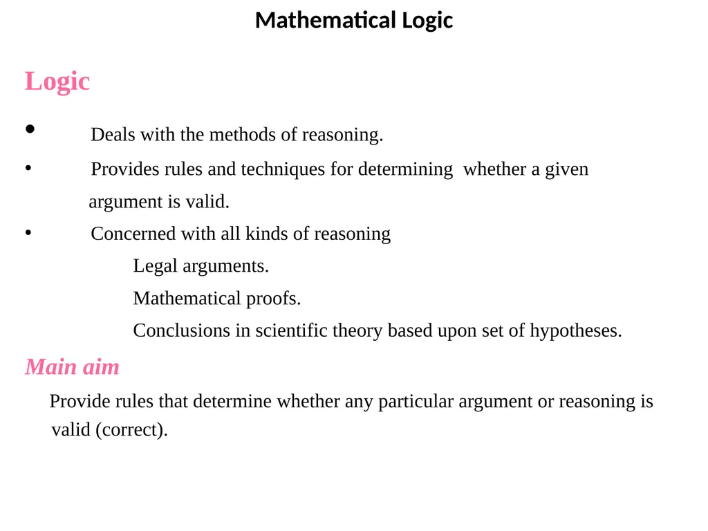
slide3. Mathematical Logic Logic
Deals with the methods of reasoning.
Provides rules and techniques for determining whether a given
argument is valid.
Concerned with all kinds of reasoning
Legal arguments.
Mathematical proofs.
Conclusions in scientific theory based upon set of hypotheses.
Main aim
Provide rules that determine whether any particular argument or reasoning is valid (correct).<br>
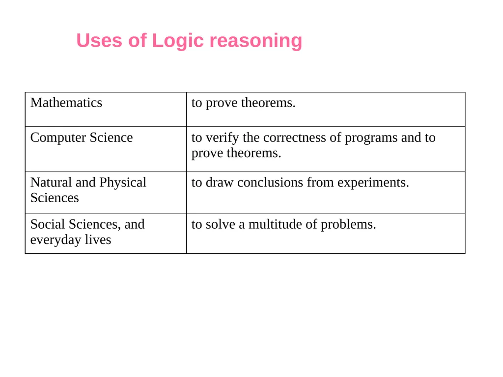
slide4. Uses of Logic reasoning<br>
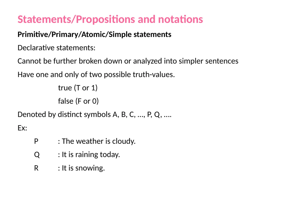
slide5. Statements/Propositions and notations
Primitive/Primary/Atomic/Simple statements
Declarative statements:
Cannot be further broken down or analyzed into simpler sentences
Have one and only of two possible truth-values.
true (T or 1)
false (F or 0)
Denoted by distinct symbols A, B, C, …, P, Q, ….
Ex:
P : The weather is cloudy.
Q : It is raining today.
R : It is snowing.<br>
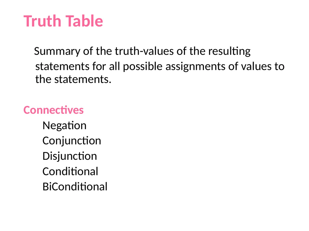
slide6. Truth Table
Summary of the truth-values of the resulting statements for all possible assignments of values to the statements.

Connectives
Negation
Conjunction
Disjunction
Conditional
BiConditional<br>
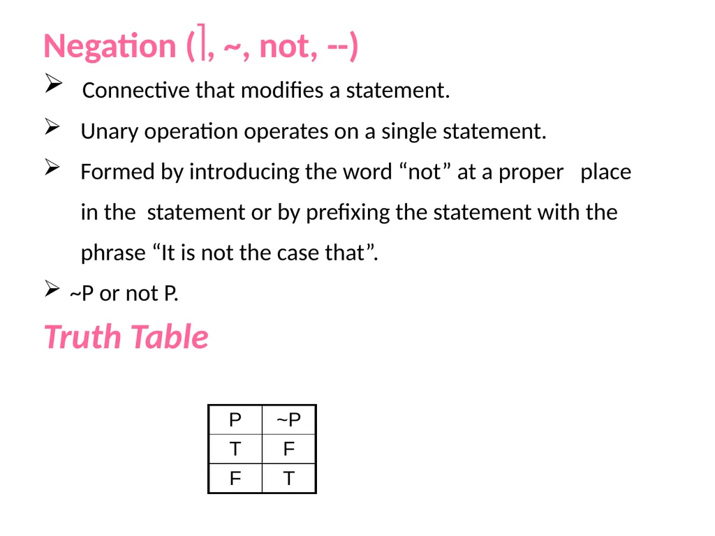
slide7. Negation (, ~, not, --)
Connective that modifies a statement.
Unary operation operates on a single statement.
Formed by introducing the word “not” at a proper place
in the statement or by prefixing the statement with the
phrase “It is not the case that”.
~P or not P.
Truth Table<br>
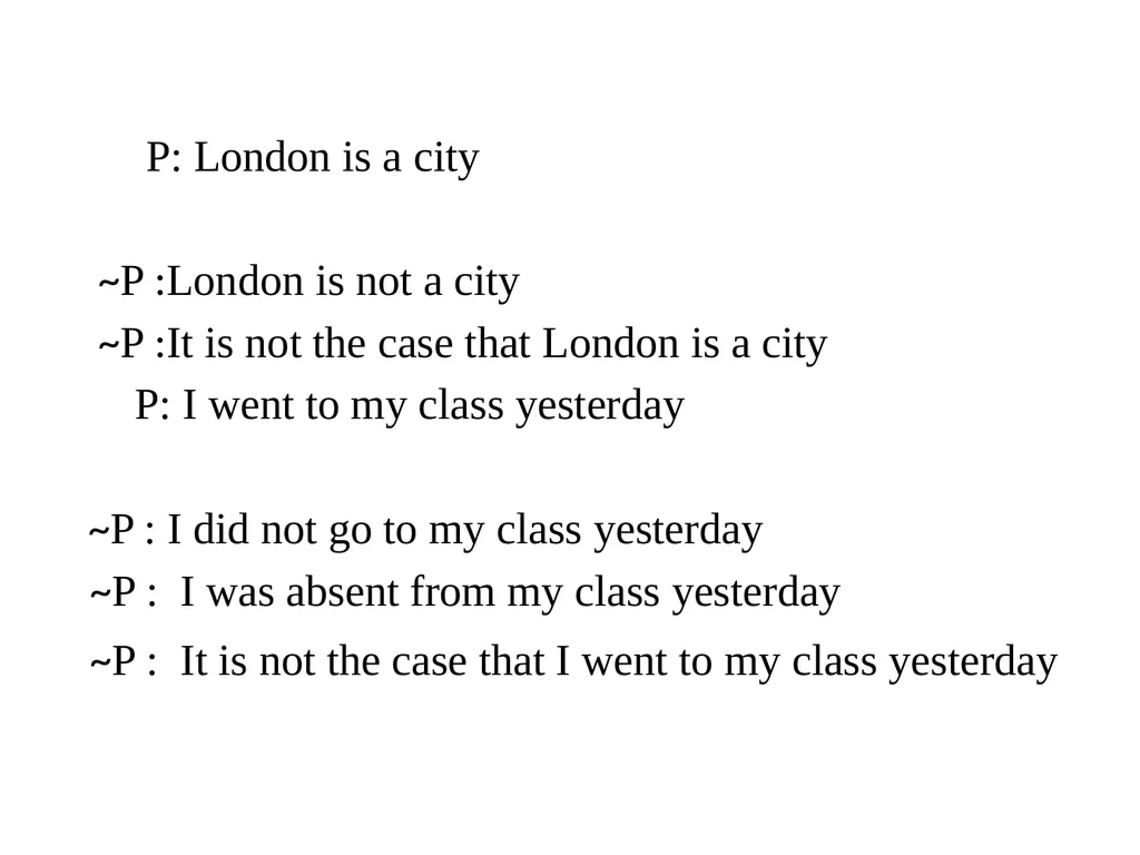
slide8. P: London is a city

~P :London is not a city
~P :It is not the case that London is a city
P: I went to my class yesterday

~P : I did not go to my class yesterday
~P : I was absent from my class yesterday
~P : It is not the case that I went to my class yesterday<br>
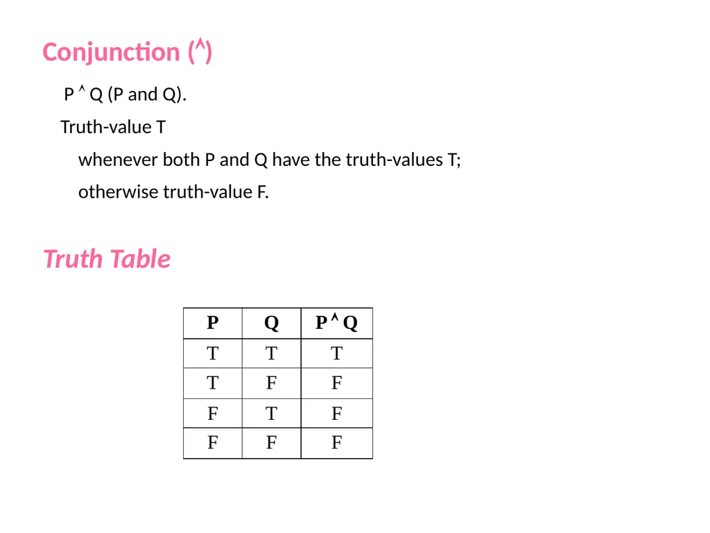
slide9. Conjunction ()
P  Q (P and Q).
Truth-value T
whenever both P and Q have the truth-values T;
otherwise truth-value F.

Truth Table<br>
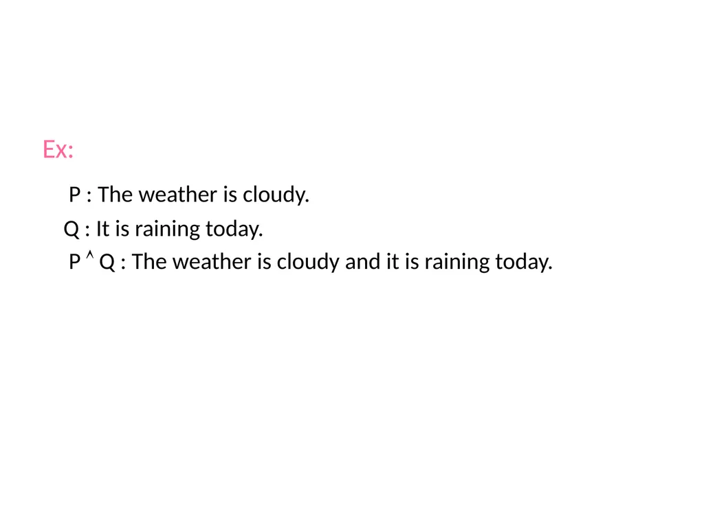
slide10. Ex:
P : The weather is cloudy.
Q : It is raining today.
P  Q : The weather is cloudy and it is raining today.<br>
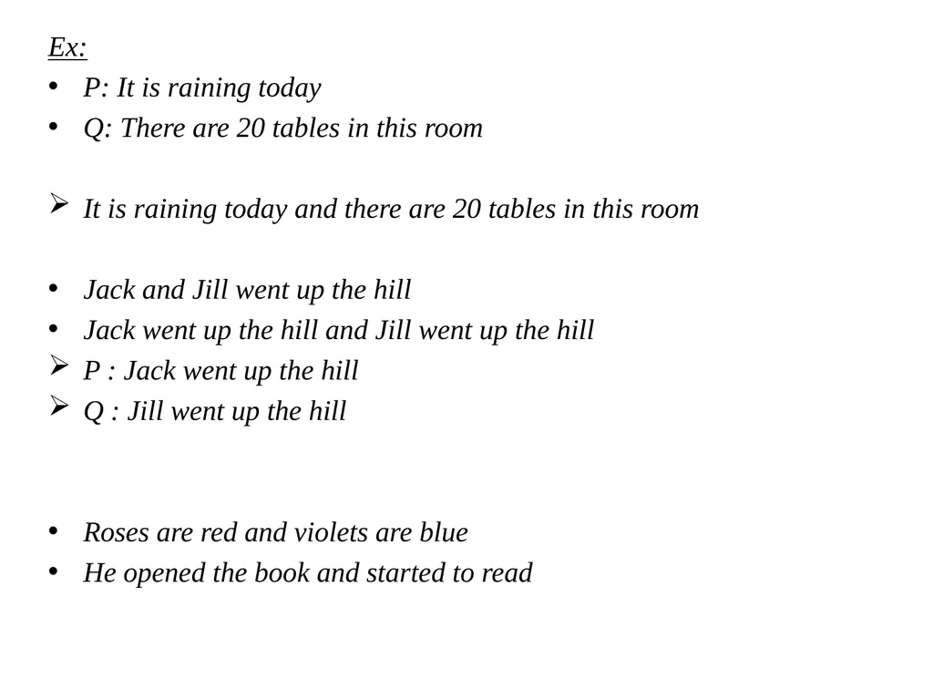
slide11. Ex:
P: It is raining today
Q: There are 20 tables in this room

It is raining today and there are 20 tables in this room

Jack and Jill went up the hill
Jack went up the hill and Jill went up the hill
P : Jack went up the hill
Q : Jill went up the hill

Roses are red and violets are blue
He opened the book and started to read<br>
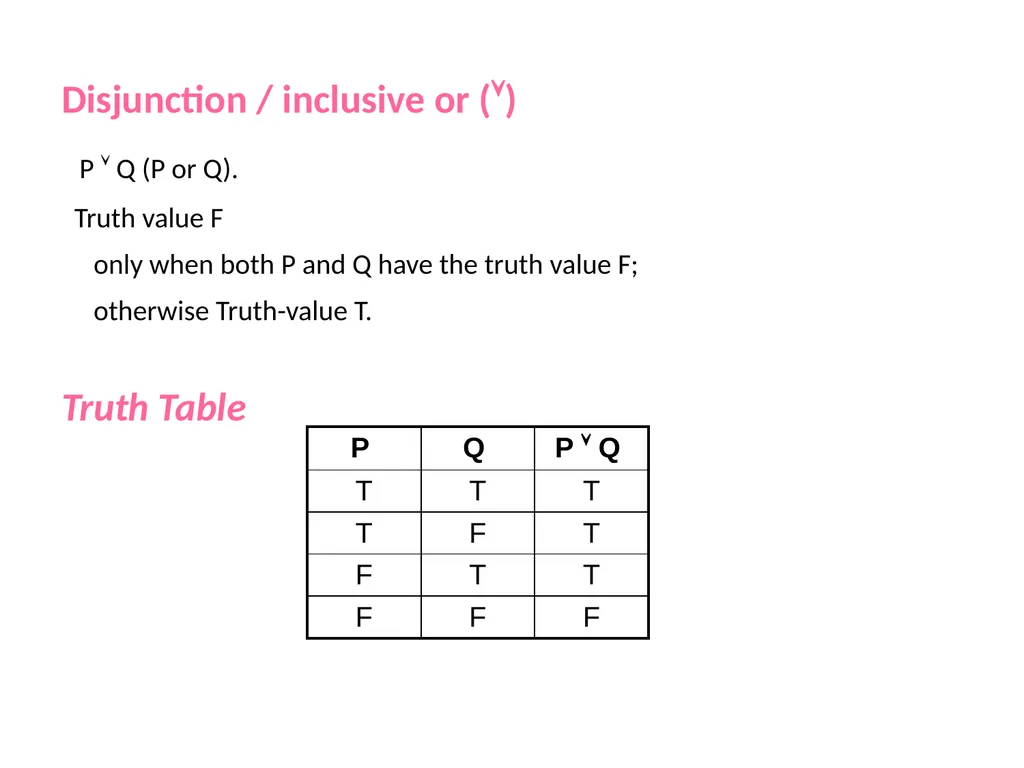
slide12. Disjunction / inclusive or ()
P  Q (P or Q).
Truth value F
only when both P and Q have the truth value F;
otherwise Truth-value T.

Truth Table<br>
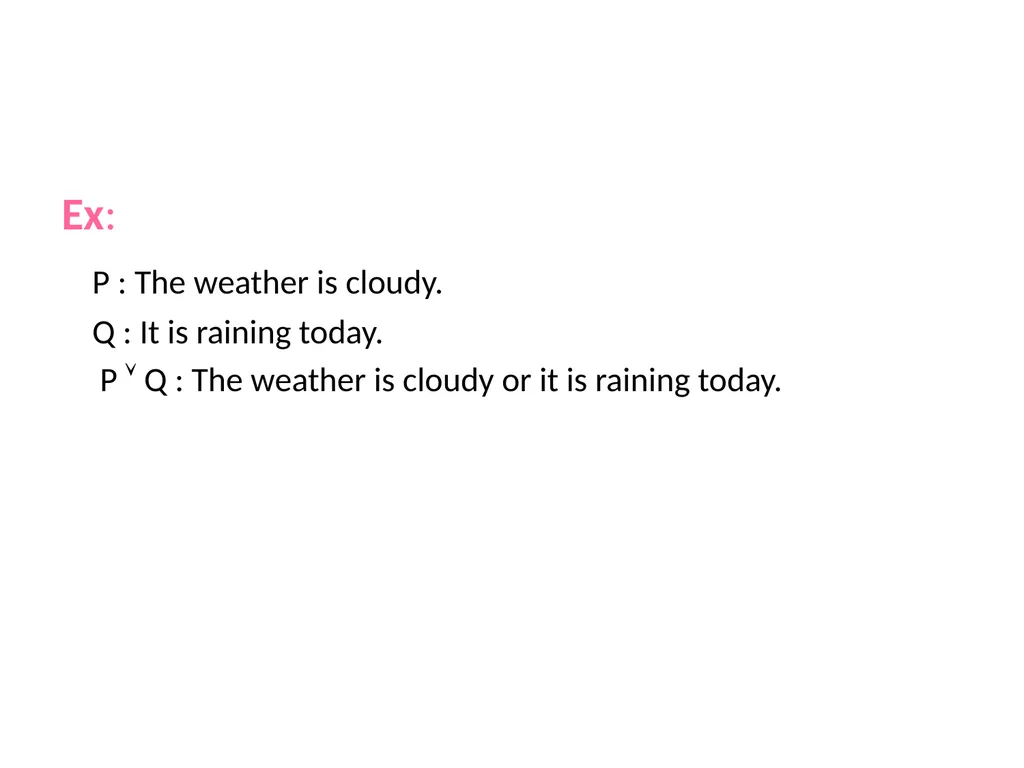
slide13. Ex:
P : The weather is cloudy.
Q : It is raining today.
P  Q : The weather is cloudy or it is raining today.<br>
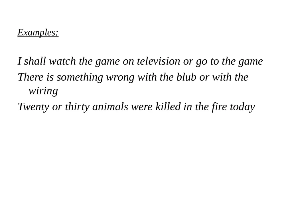
slide14. Examples:

I shall watch the game on television or go to the game
There is something wrong with the blub or with the wiring
Twenty or thirty animals were killed in the fire today<br>
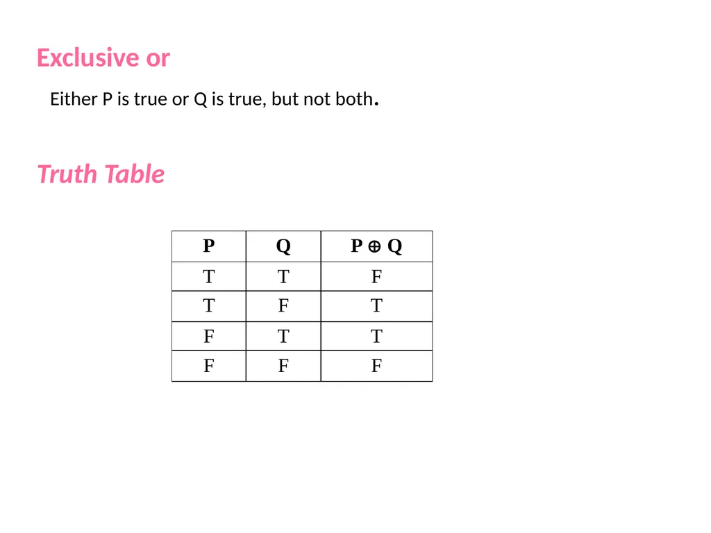
slide15. Exclusive or
Either P is true or Q is true, but not both.

Truth Table<br>
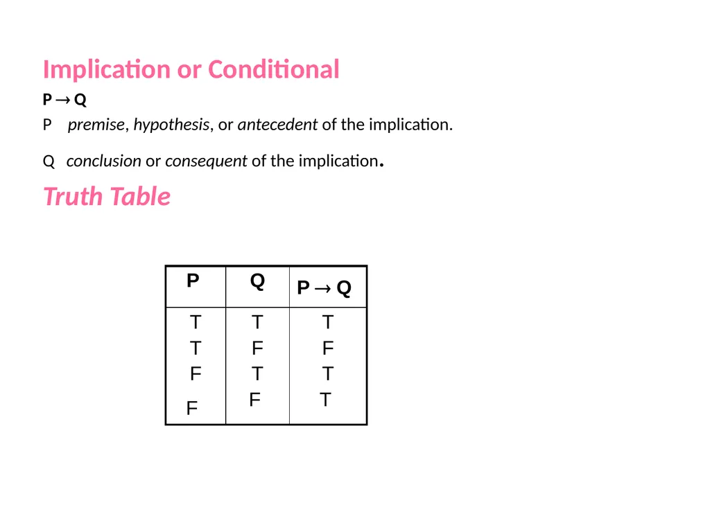
slide16. Implication or Conditional
P  Q
P premise, hypothesis, or antecedent of the implication.
Q conclusion or consequent of the implication.
Truth Table<br>
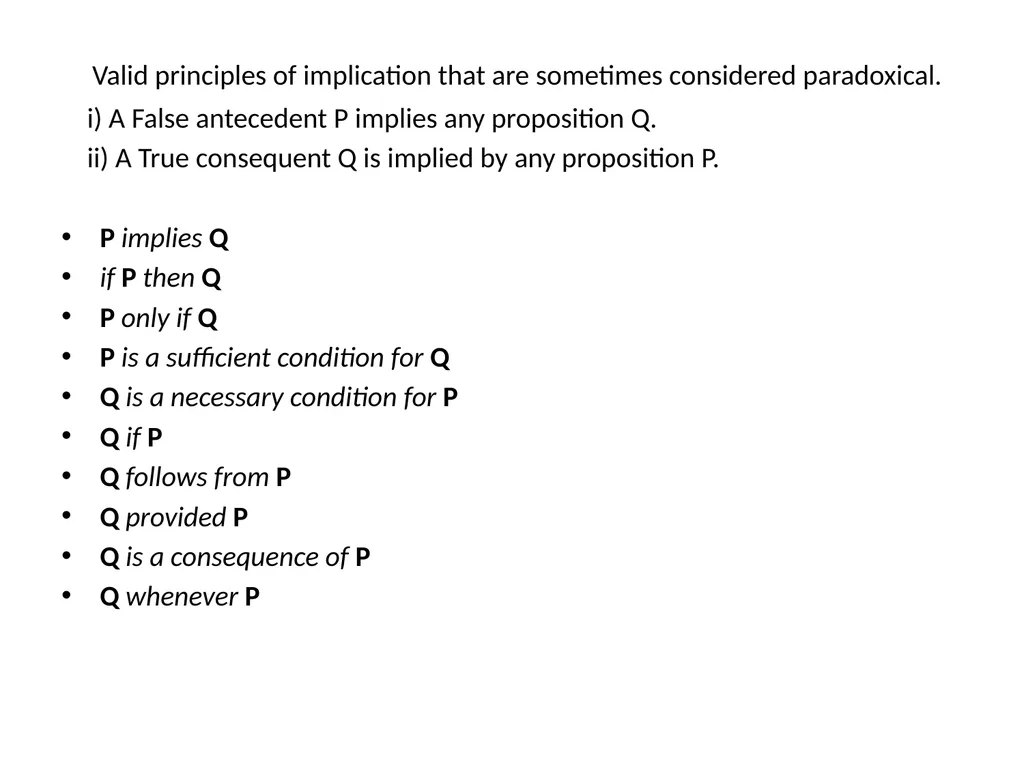
slide17. Valid principles of implication that are sometimes considered paradoxical.
i) A False antecedent P implies any proposition Q.
ii) A True consequent Q is implied by any proposition P.

P implies Q
if P then Q
P only if Q
P is a sufficient condition for Q
Q is a necessary condition for P
Q if P
Q follows from P
Q provided P
Q is a consequence of P
Q whenever P<br>
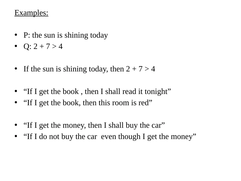
slide18. Examples:

P: the sun is shining today
Q: 2 + 7 > 4

If the sun is shining today, then 2 + 7 > 4

“If I get the book , then I shall read it tonight”
“If I get the book, then this room is red”

“If I get the money, then I shall buy the car”
“If I do not buy the car even though I get the money”<br>
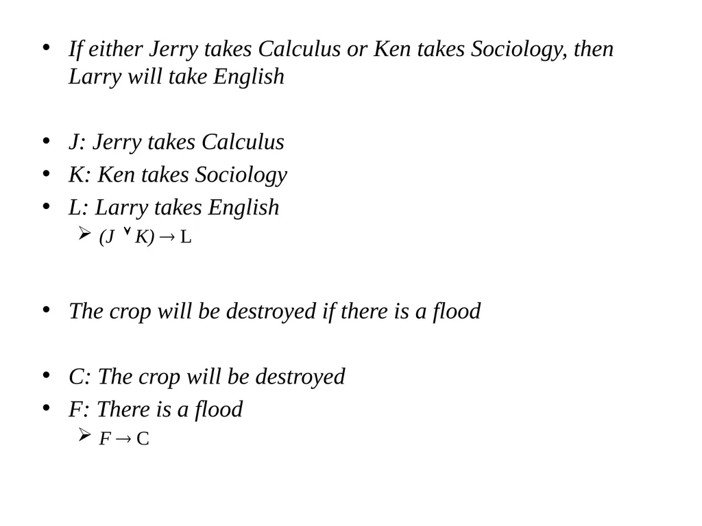
slide19. If either Jerry takes Calculus or Ken takes Sociology, then Larry will take English

J: Jerry takes Calculus
K: Ken takes Sociology
L: Larry takes English
(J  K)  L

The crop will be destroyed if there is a flood

C: The crop will be destroyed
F: There is a flood
F  C<br>
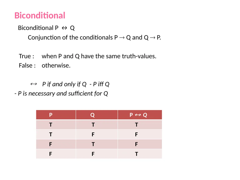
slide20. Biconditional
Biconditional P ↔ Q
Conjunction of the conditionals P  Q and Q  P.

True : when P and Q have the same truth-values.
False : otherwise.

 P if and only if Q - P iff Q
- P is necessary and sufficient for Q<br>
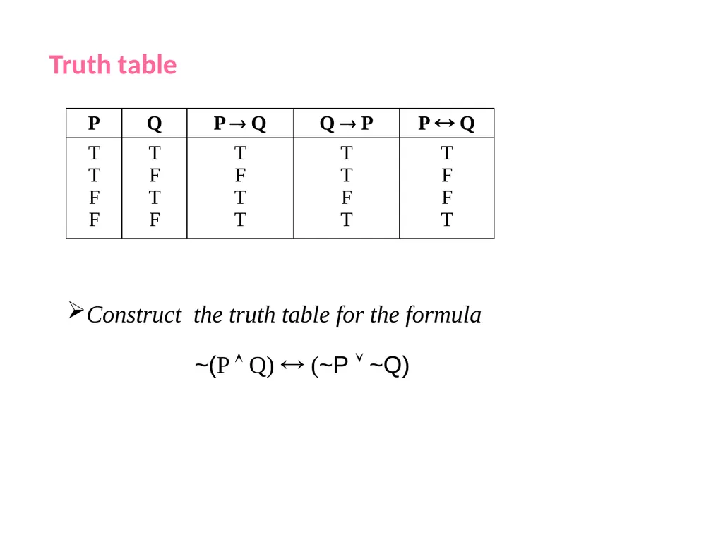
slide21. Truth table Construct the truth table for the formula

~(P  Q)  (~P  ~Q)<br>
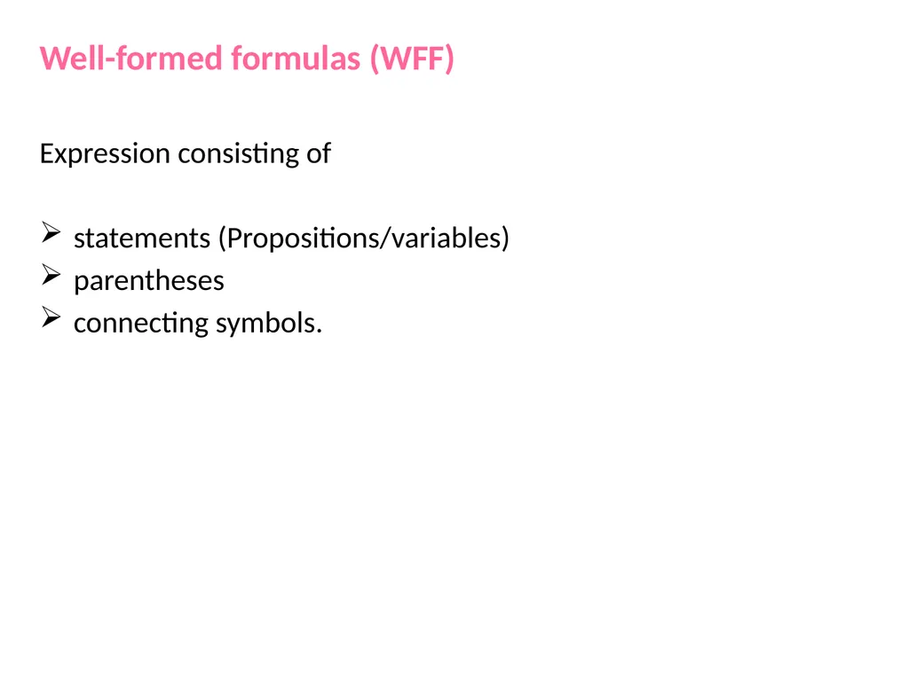
slide22. Well-formed formulas (WFF)

Expression consisting of

statements (Propositions/variables)
parentheses
connecting symbols.<br>
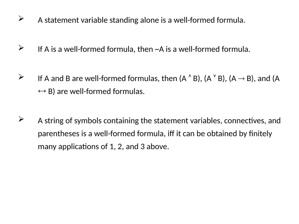
slide23. A statement variable standing alone is a well-formed formula.

If A is a well-formed formula, then ~A is a well-formed formula.

If A and B are well-formed formulas, then (A  B), (A  B), (A  B), and (A  B) are well-formed formulas.

A string of symbols containing the statement variables, connectives, and parentheses is a well-formed formula, iff it can be obtained by finitely many applications of 1, 2, and 3 above.<br>
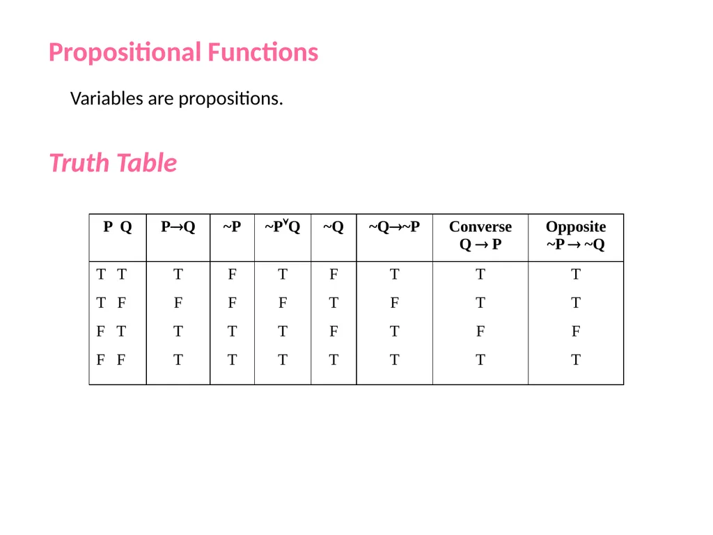
slide24. Propositional Functions
Variables are propositions.

Truth Table<br>
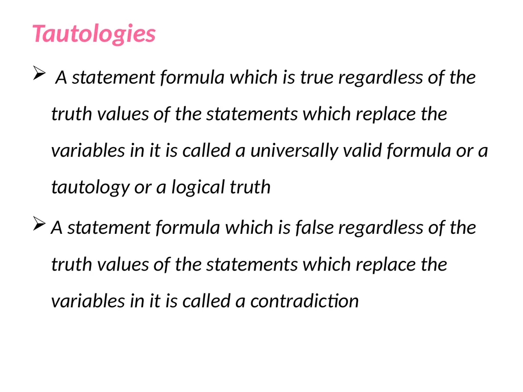
slide25. Tautologies
A statement formula which is true regardless of the truth values of the statements which replace the variables in it is called a universally valid formula or a tautology or a logical truth
A statement formula which is false regardless of the truth values of the statements which replace the variables in it is called a contradiction<br>
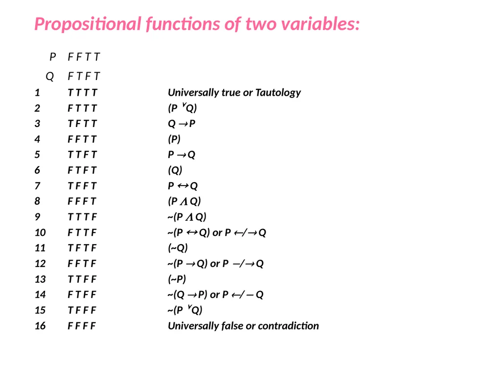
slide26. Propositional functions of two variables:
P F F T T
Q F T F T
T T T T Universally true or Tautology
F T T T (P  Q)
3 T F T T Q  P
4 F F T T (P)
5 T T F T P  Q
6 F T F T (Q)
7 T F F T P  Q
8 F F F T (P  Q)
9 T T T F ~(P  Q)
10 F T T F ~(P  Q) or P / Q
11 T F T F (~Q)
12 F F T F ~(P  Q) or P / Q
13 T T F F (~P)
14 F T F F ~(Q  P) or P / Q
15 T F F F ~(P  Q)
16 F F F F Universally false or contradiction<br>
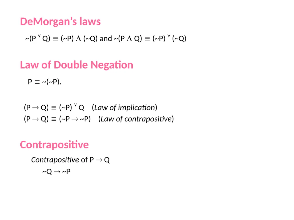
slide27. DeMorgan’s laws
~(P  Q)  (~P)  (~Q) and ~(P  Q)  (~P)  (~Q)

Law of Double Negation
P  ~(~P).

(P  Q)  (~P)  Q (Law of implication)
(P  Q)  (~P  ~P) (Law of contrapositive)

Contrapositive
Contrapositive of P  Q
~Q  ~P<br>
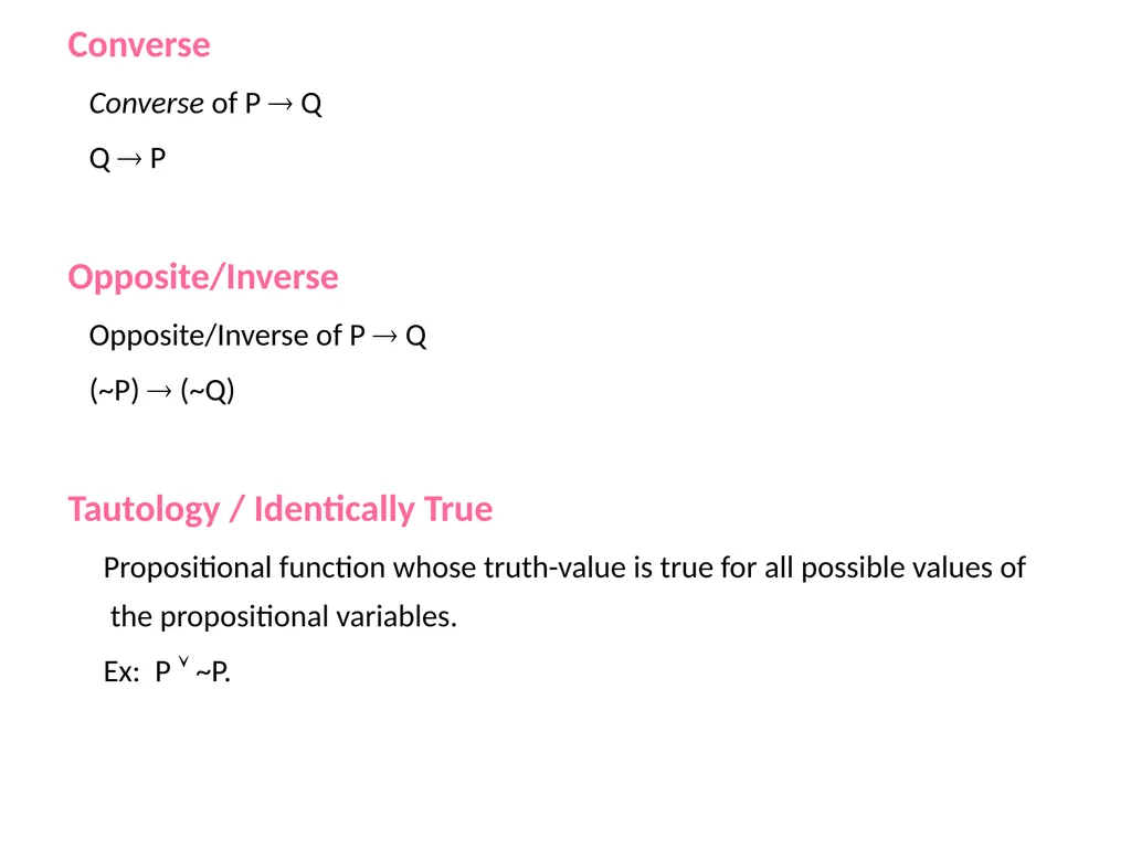
slide28. Converse
Converse of P  Q
Q  P

Opposite/Inverse
Opposite/Inverse of P  Q
(~P)  (~Q)

Tautology / Identically True
Propositional function whose truth-value is true for all possible values of the propositional variables.
Ex: P  ~P.<br>
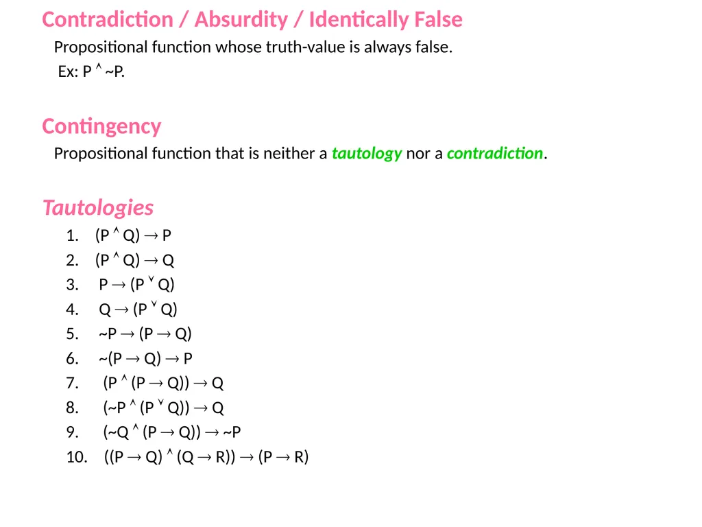
slide29. Contradiction / Absurdity / Identically False
Propositional function whose truth-value is always false.
Ex: P  ~P.

Contingency
Propositional function that is neither a tautology nor a contradiction.

Tautologies
1. (P  Q)  P
2. (P  Q)  Q
3. P  (P  Q)
4. Q  (P  Q)
5. ~P  (P  Q)
6. ~(P  Q)  P
7. (P  (P  Q))  Q
8. (~P  (P  Q))  Q
9. (~Q  (P  Q))  ~P
10. ((P  Q)  (Q  R))  (P  R)<br>
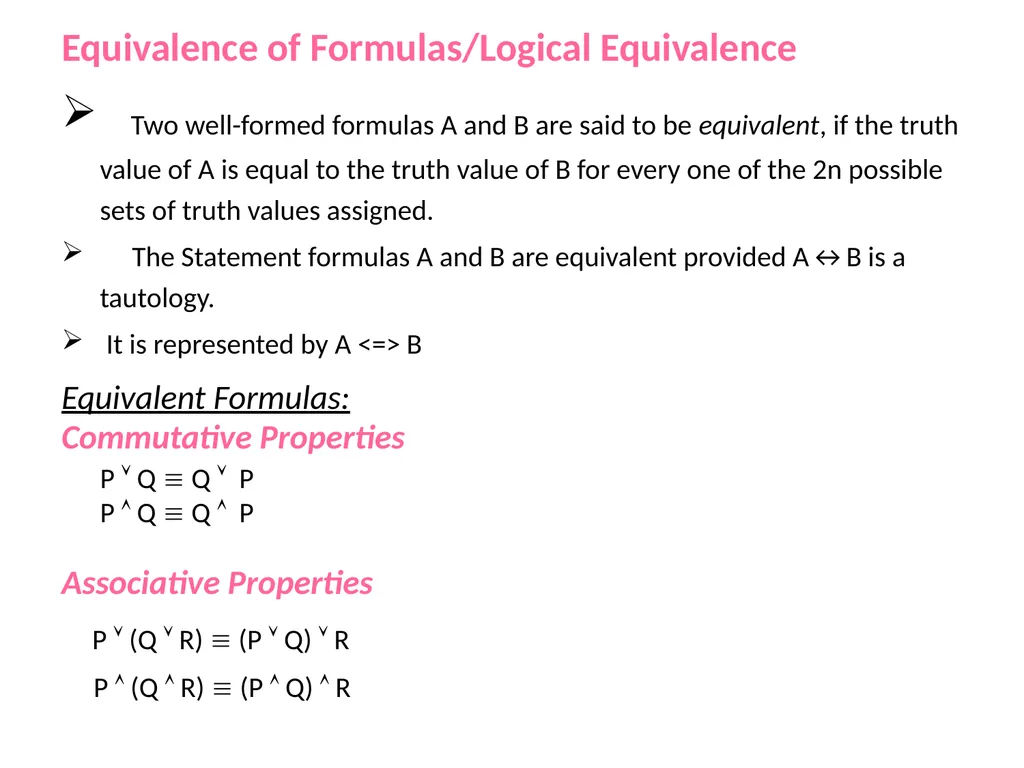
slide30. Equivalence of Formulas/Logical Equivalence
Two well-formed formulas A and B are said to be equivalent, if the truth value of A is equal to the truth value of B for every one of the 2n possible sets of truth values assigned.
The Statement formulas A and B are equivalent provided A↔B is a tautology.
It is represented by A <=> B
Equivalent Formulas:
Commutative Properties
P  Q  Q  P
P  Q  Q  P

Associative Properties
P  (Q  R)  (P  Q)  R
P  (Q  R)  (P  Q)  R<br>
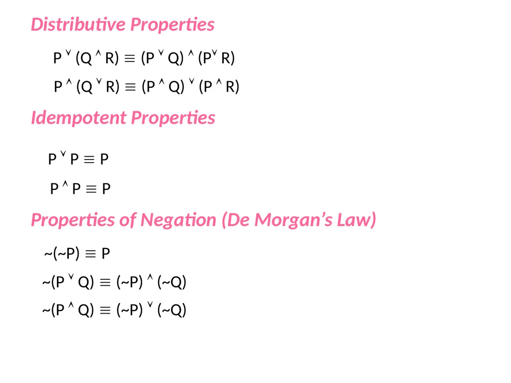
slide31. Distributive Properties
P  (Q  R)  (P  Q)  (P R)
P  (Q  R)  (P  Q)  (P  R)
Idempotent Properties
P  P  P
P  P  P
Properties of Negation (De Morgan’s Law)
~(~P)  P
~(P  Q)  (~P)  (~Q)
~(P  Q)  (~P)  (~Q)<br>
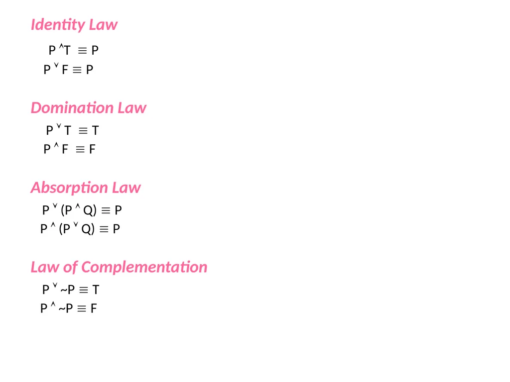
slide32. Identity Law
P T  P
P  F  P

Domination Law
P  T  T
P  F  F

Absorption Law
P  (P  Q)  P
P  (P  Q)  P

Law of Complementation
P  ~P  T
P  ~P  F<br>
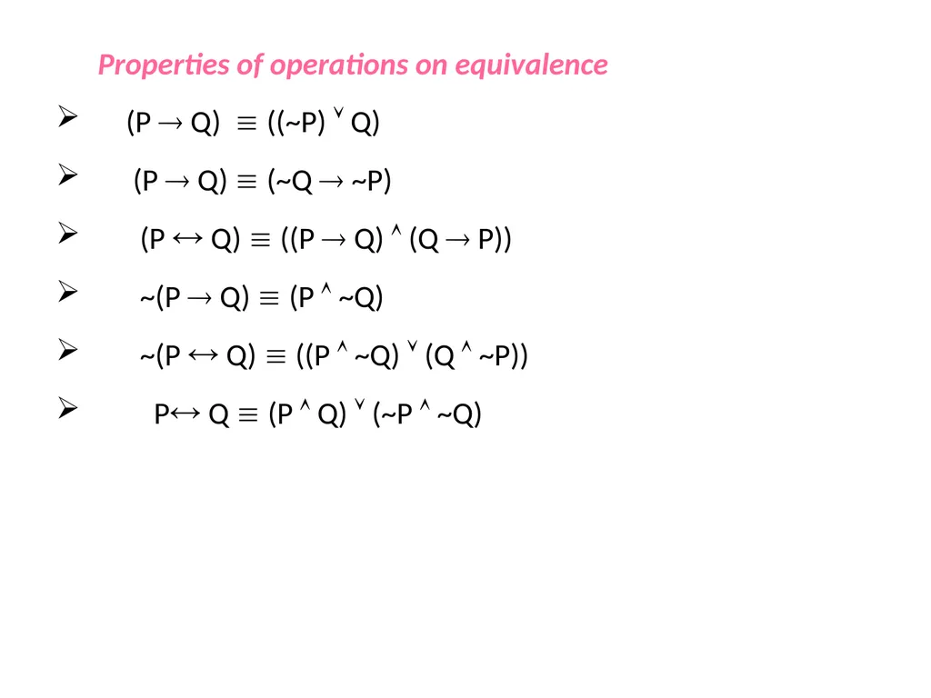
slide33. Properties of operations on equivalence
(P  Q)  ((~P)  Q)
(P  Q)  (~Q  ~P)
(P  Q)  ((P  Q)  (Q  P))
~(P  Q)  (P  ~Q)
~(P  Q)  ((P  ~Q)  (Q  ~P))
P Q  (P  Q)  (~P  ~Q)<br>
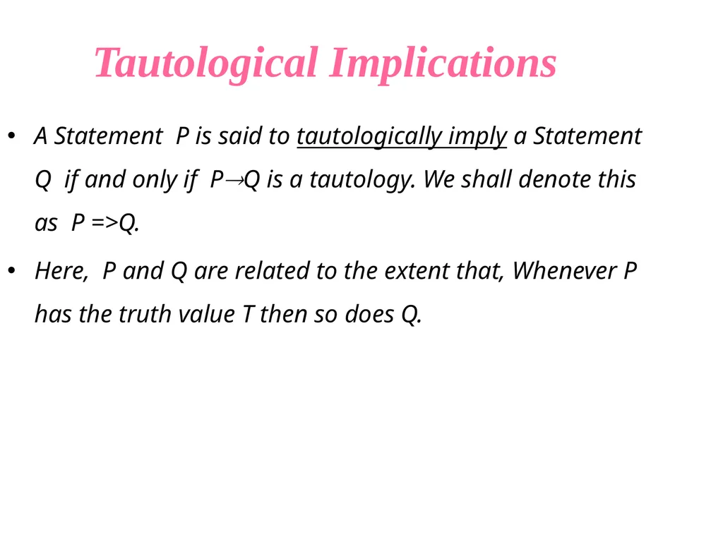
slide34. Tautological Implications A Statement P is said to tautologically imply a Statement Q if and only if PQ is a tautology. We shall denote this as P =>Q.
Here, P and Q are related to the extent that, Whenever P has the truth value T then so does Q.<br>
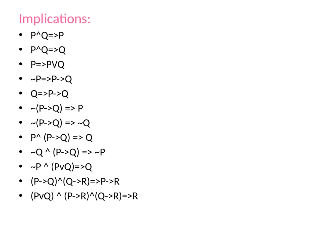
slide35. Implications:
P^Q=>P
P^Q=>Q
P=>PVQ
~P=>P->Q
Q=>P->Q
~(P->Q) => P
~(P->Q) => ~Q
P^ (P->Q) => Q
~Q ^ (P->Q) => ~P
~P ^ (PvQ)=>Q
(P->Q)^(Q->R)=>P->R
(PvQ) ^ (P->R)^(Q->R)=>R<br>
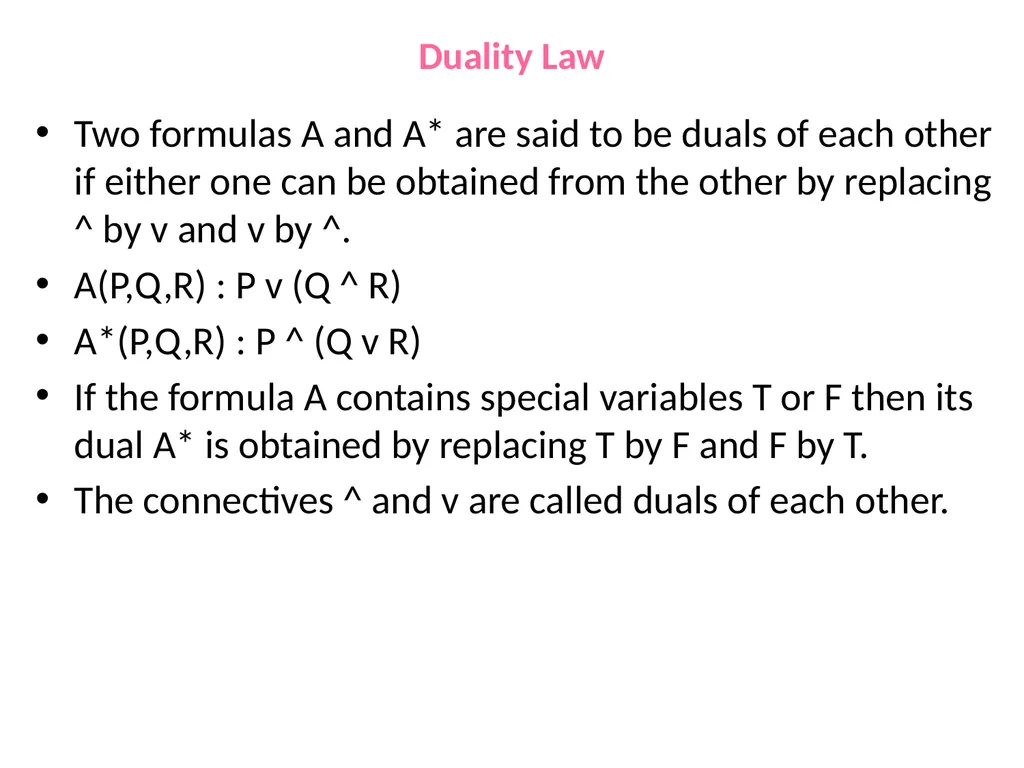
slide36. Duality Law Two formulas A and A* are said to be duals of each other if either one can be obtained from the other by replacing ^ by v and v by ^.
A(P,Q,R) : P v (Q ^ R)
A*(P,Q,R) : P ^ (Q v R)
If the formula A contains special variables T or F then its dual A* is obtained by replacing T by F and F by T.
The connectives ^ and v are called duals of each other.<br>
slide37. Theorem
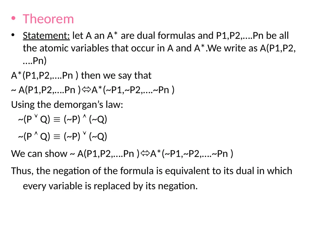
Statement: let A an A* are dual formulas and P1,P2,….Pn be all the atomic variables that occur in A and A*.We write as A(P1,P2,….Pn)
A*(P1,P2,….Pn ) then we say that
~ A(P1,P2,….Pn )A*(~P1,~P2,….~Pn )
Using the demorgan’s law:
~(P  Q)  (~P)  (~Q)
~(P  Q)  (~P)  (~Q)
We can show ~ A(P1,P2,….Pn )A*(~P1,~P2,….~Pn )
Thus, the negation of the formula is equivalent to its dual in which every variable is replaced by its negation.<br>
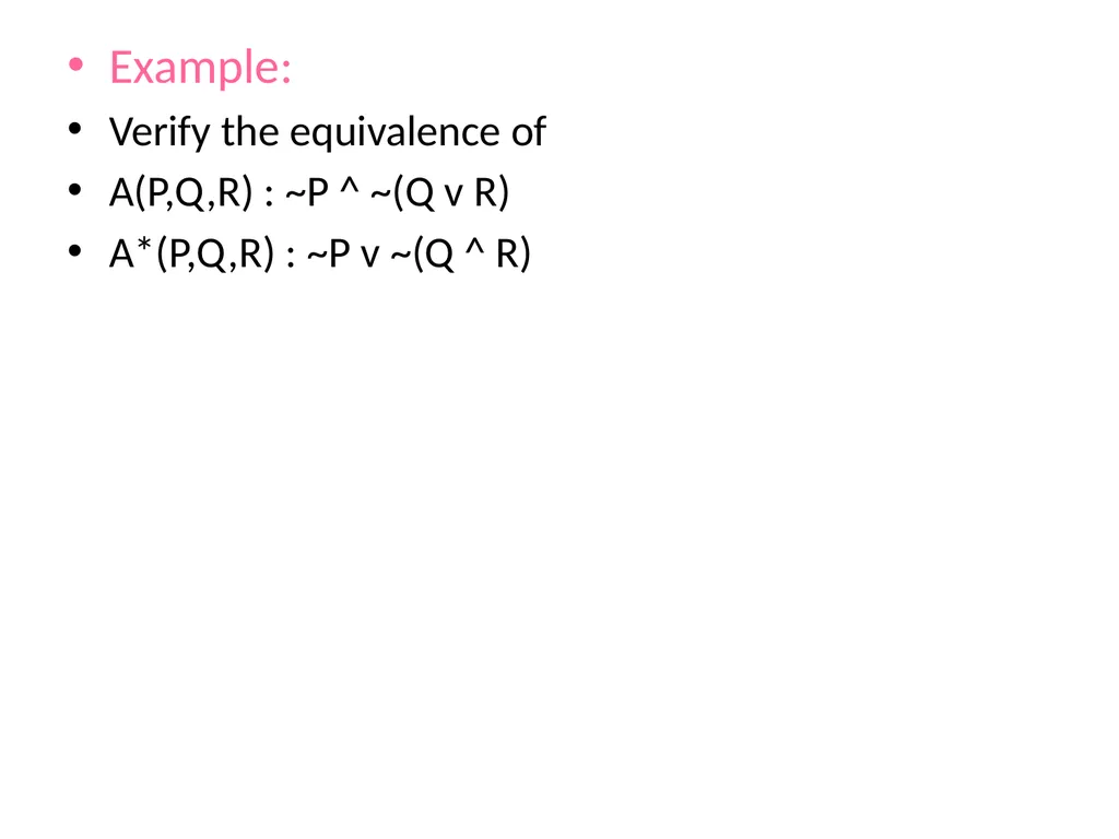
slide38. Example:
Verify the equivalence of
A(P,Q,R) : ~P ^ ~(Q v R)
A*(P,Q,R) : ~P v ~(Q ^ R)<br>
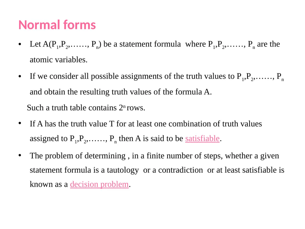
slide39. Normal forms
Let A(P1,P2,……, Pn) be a statement formula where P1,P2,……, Pn are the atomic variables.
If we consider all possible assignments of the truth values to P1,P2,……, Pn and obtain the resulting truth values of the formula A.
Such a truth table contains 2n rows.
If A has the truth value T for at least one combination of truth values assigned to P1,P2,……, Pn then A is said to be satisfiable.
The problem of determining , in a finite number of steps, whether a given statement formula is a tautology or a contradiction or at least satisfiable is known as a decision problem.<br>
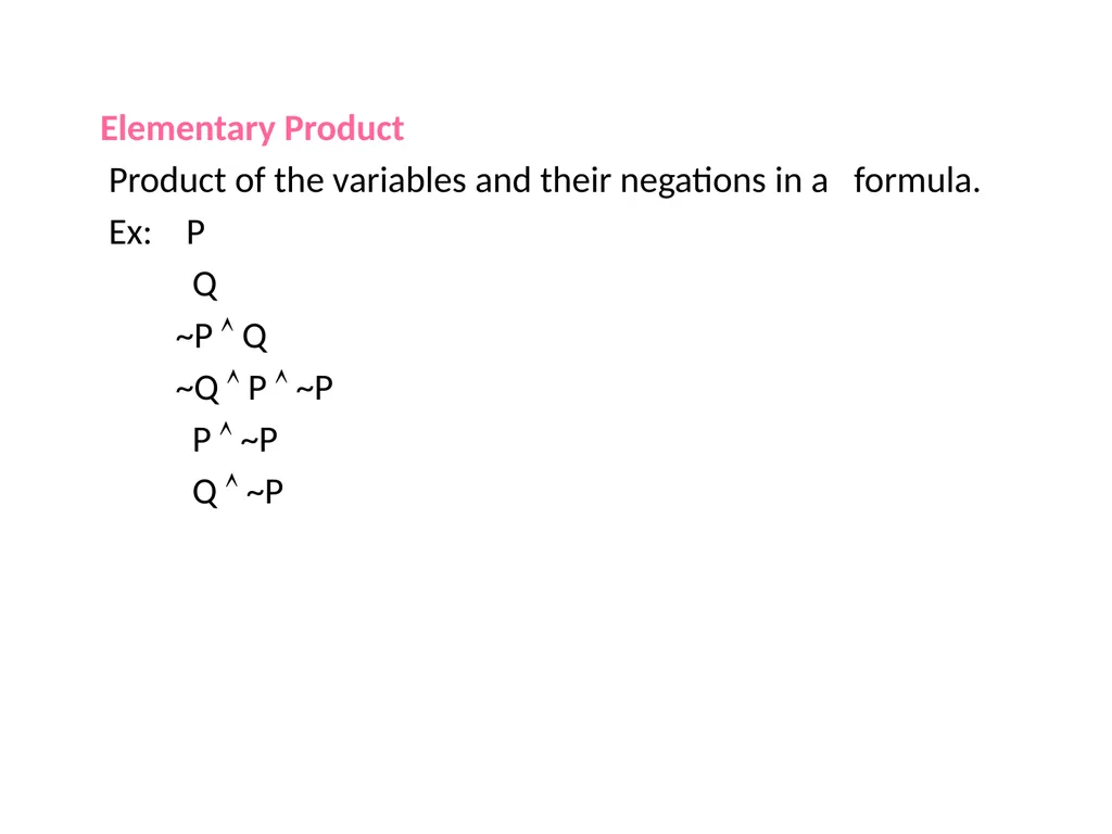
slide40. Elementary Product
Product of the variables and their negations in a formula.
Ex: P
Q
~P  Q
~Q  P  ~P
P  ~P
Q  ~P<br>
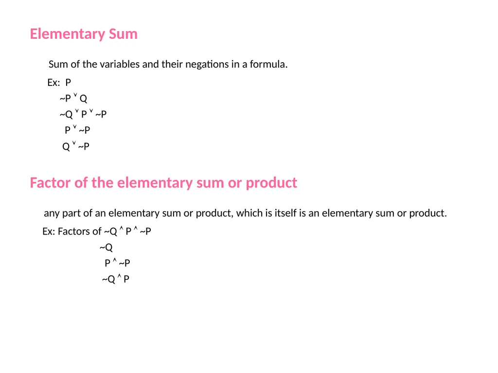
slide41. Elementary Sum
Sum of the variables and their negations in a formula.
Ex: P
~P  Q
~Q  P  ~P
P  ~P
Q  ~P

Factor of the elementary sum or product
any part of an elementary sum or product, which is itself is an elementary sum or product.
Ex: Factors of ~Q  P  ~P
~Q
P  ~P
~Q  P<br>
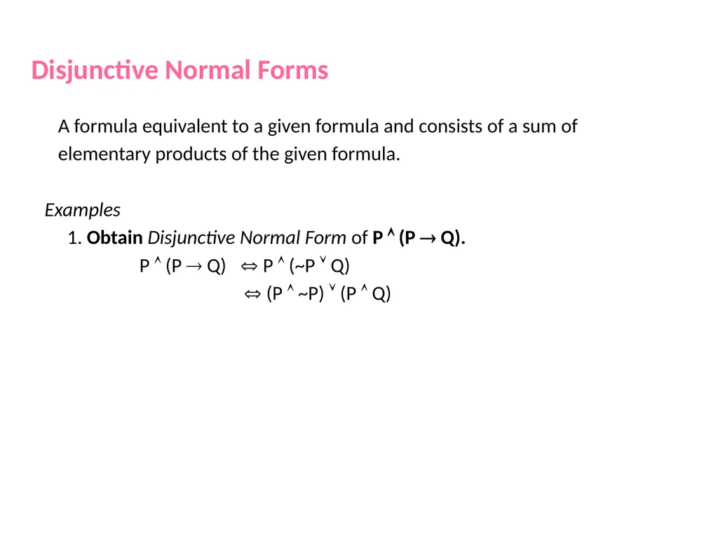
slide42. Disjunctive Normal Forms
A formula equivalent to a given formula and consists of a sum of elementary products of the given formula.

Examples
1. Obtain Disjunctive Normal Form of P  (P  Q).
P  (P  Q)  P  (~P  Q)
 (P  ~P)  (P  Q)<br>
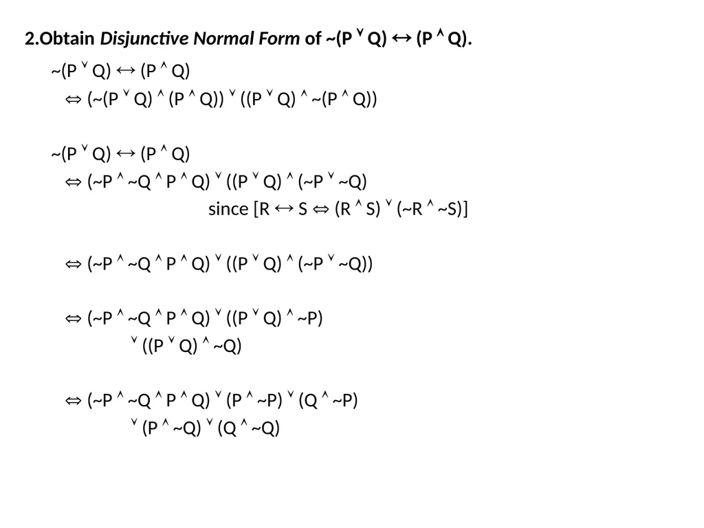
slide43. 2.Obtain Disjunctive Normal Form of ~(P  Q)  (P  Q).
~(P  Q)  (P  Q)
 (~(P  Q)  (P  Q))  ((P  Q)  ~(P  Q))

~(P  Q)  (P  Q)
 (~P  ~Q  P  Q)  ((P  Q)  (~P  ~Q)
since [R  S  (R  S)  (~R  ~S)]

 (~P  ~Q  P  Q)  ((P  Q)  (~P  ~Q))

 (~P  ~Q  P  Q)  ((P  Q)  ~P)
 ((P  Q)  ~Q)

 (~P  ~Q  P  Q)  (P  ~P)  (Q  ~P)
 (P  ~Q)  (Q  ~Q)<br>
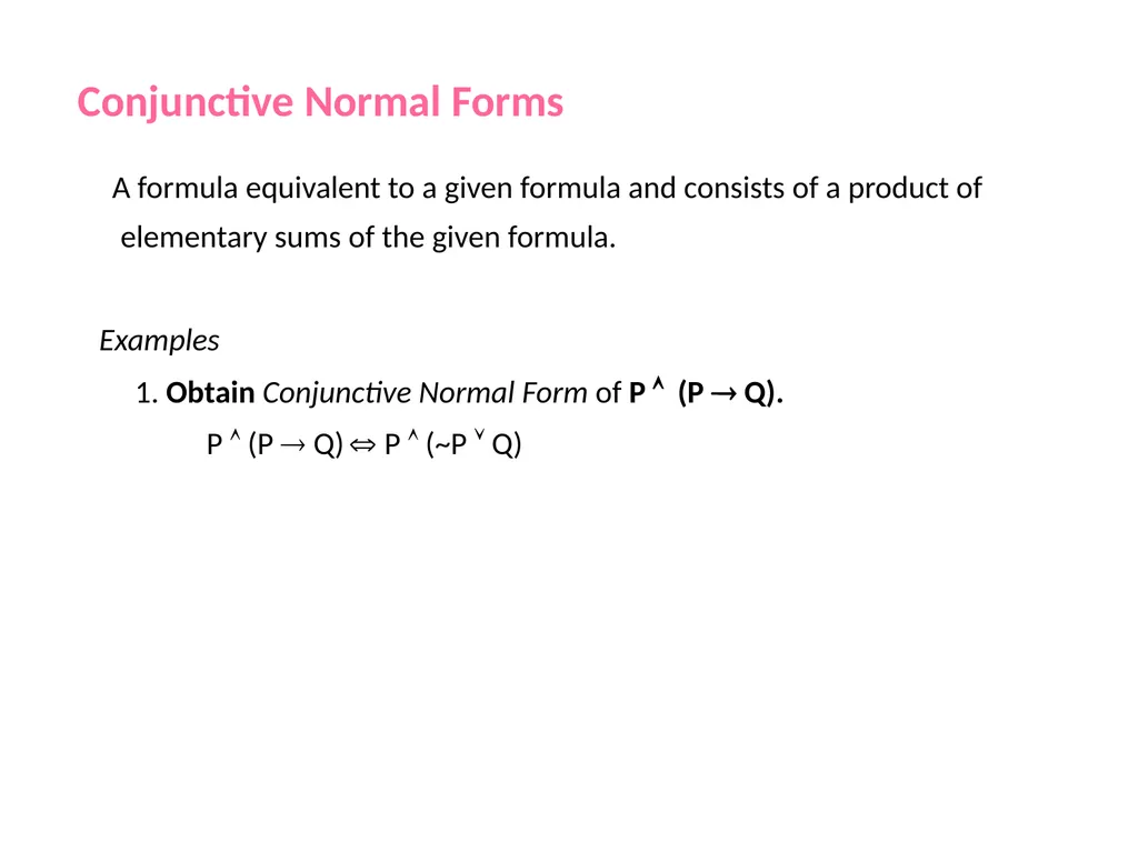
slide44. Conjunctive Normal Forms
A formula equivalent to a given formula and consists of a product of elementary sums of the given formula.

Examples
1. Obtain Conjunctive Normal Form of P  (P  Q).
P  (P  Q)  P  (~P  Q)<br>
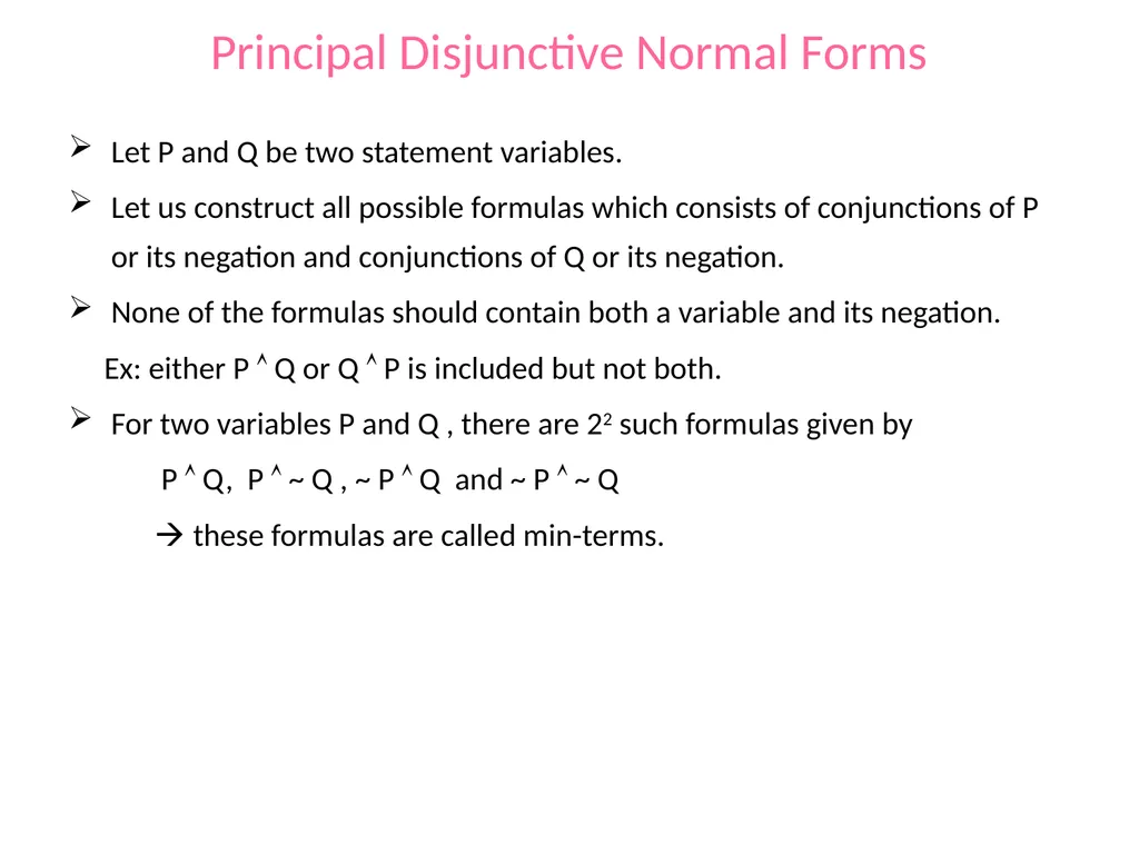
slide45. Principal Disjunctive Normal Forms Let P and Q be two statement variables.
Let us construct all possible formulas which consists of conjunctions of P or its negation and conjunctions of Q or its negation.
None of the formulas should contain both a variable and its negation.
Ex: either P  Q or Q  P is included but not both.
For two variables P and Q , there are 22 such formulas given by
P  Q, P  ~ Q , ~ P  Q and ~ P  ~ Q
 these formulas are called min-terms.<br>
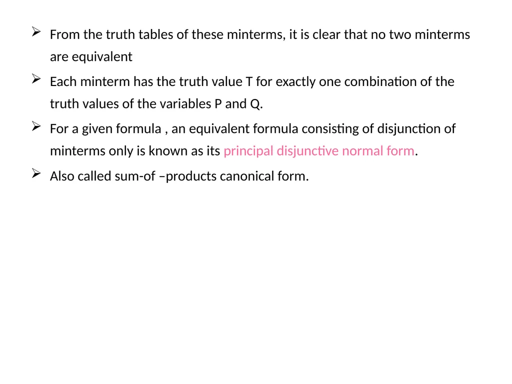
slide46. From the truth tables of these minterms, it is clear that no two minterms are equivalent
Each minterm has the truth value T for exactly one combination of the truth values of the variables P and Q.
For a given formula , an equivalent formula consisting of disjunction of minterms only is known as its principal disjunctive normal form.
Also called sum-of –products canonical form.<br>
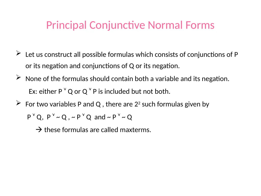
slide47. Principal Conjunctive Normal Forms Let us construct all possible formulas which consists of conjunctions of P or its negation and conjunctions of Q or its negation.
None of the formulas should contain both a variable and its negation.
Ex: either P  Q or Q  P is included but not both.
For two variables P and Q , there are 22 such formulas given by
P  Q, P  ~ Q , ~ P  Q and ~ P  ~ Q
 these formulas are called maxterms.<br>
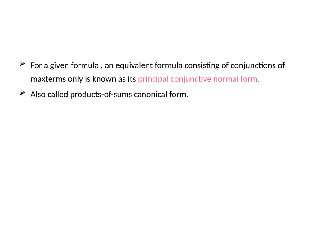
slide48. For a given formula , an equivalent formula consisting of conjunctions of maxterms only is known as its principal conjunctive normal form.
Also called products-of-sums canonical form.<br>
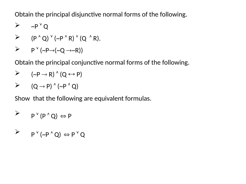
slide49. Obtain the principal disjunctive normal forms of the following.
~P  Q
(P  Q)  (~P  R)  (Q  R).
P  (~P(~Q ~R))
Obtain the principal conjunctive normal forms of the following.
(~P  R)  (Q  P)
(Q  P)  (~P  Q)
Show that the following are equivalent formulas.
P  (P  Q)  P
P  (~P  Q)  P  Q<br>
slide50. Theory of Inference
The main function of the logic is to provide rules of inference, or principles of reasoning.
The theory associated with such rules is known as inference theory because it is concerned with the inferring of a conclusion from certain premises.
When a conclusion is derived from a set of premises by using the accepted rules of reasoning, then such a process of derivation is called a deduction or formal proof.
In a formal proof, every rule of inference that is used at any stage in the derivation is acknowledged.<br>
slide51. Theory of Inference
Now we come to the questions of what we mean by the rules and theory of inference
The rules of inference are criteria for determining the validity of an argument.
These rules are stated in terms of the forms of the statements involved rather than in terms of the actual statements or their truth values.<br>
slide52. Validity Using Truth Tables
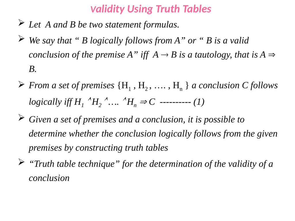
Let A and B be two statement formulas.
We say that “ B logically follows from A” or “ B is a valid conclusion of the premise A” iff A  B is a tautology, that is A  B.
From a set of premises {H1 , H2 , …. , Hn } a conclusion C follows logically iff H1  H2  ….  Hn  C ---------- (1)
Given a set of premises and a conclusion, it is possible to determine whether the conclusion logically follows from the given premises by constructing truth tables
“Truth table technique” for the determination of the validity of a conclusion<br>
slide53. Rules of Inference
Rule P: A premise may be introduced at any point in the derivation
Rule T: A formula S may be introduced in a derivation if S is tautologically implied by any one or more of the preceding formulas in the derivation<br>
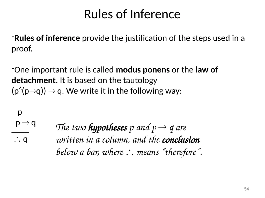
slide54. Rules of Inference Rules of inference provide the justification of the steps used in a proof.

One important rule is called modus ponens or the law of detachment. It is based on the tautology (p(pq))  q. We write it in the following way:

p
p  q
____
 q 54 The two hypotheses p and p  q are written in a column, and the conclusionbelow a bar, where  means “therefore”.<br>
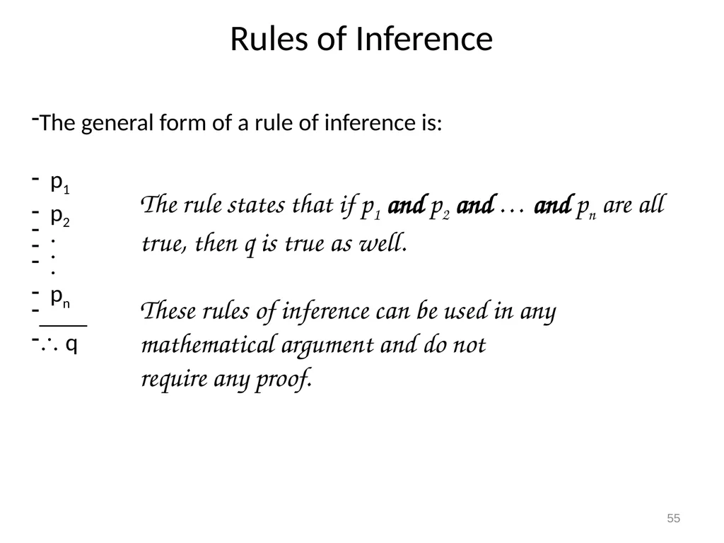
slide55. Rules of Inference The general form of a rule of inference is:

p1
p2
.
.
.
pn
____
 q 55 The rule states that if p1 and p2 and … and pn are all true, then q is true as well.

These rules of inference can be used in any mathematical argument and do not require any proof.<br>
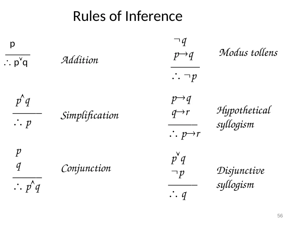
slide56. 56 Rules of Inference p
_____
 pq Addition pq
_____
 p Simplification p
q
_____
 pq Conjunction q
pq
_____
 p Modus tollens pq
qr
_____
 pr Hypothetical syllogism pq
p
_____
 q Disjunctive syllogism<br>
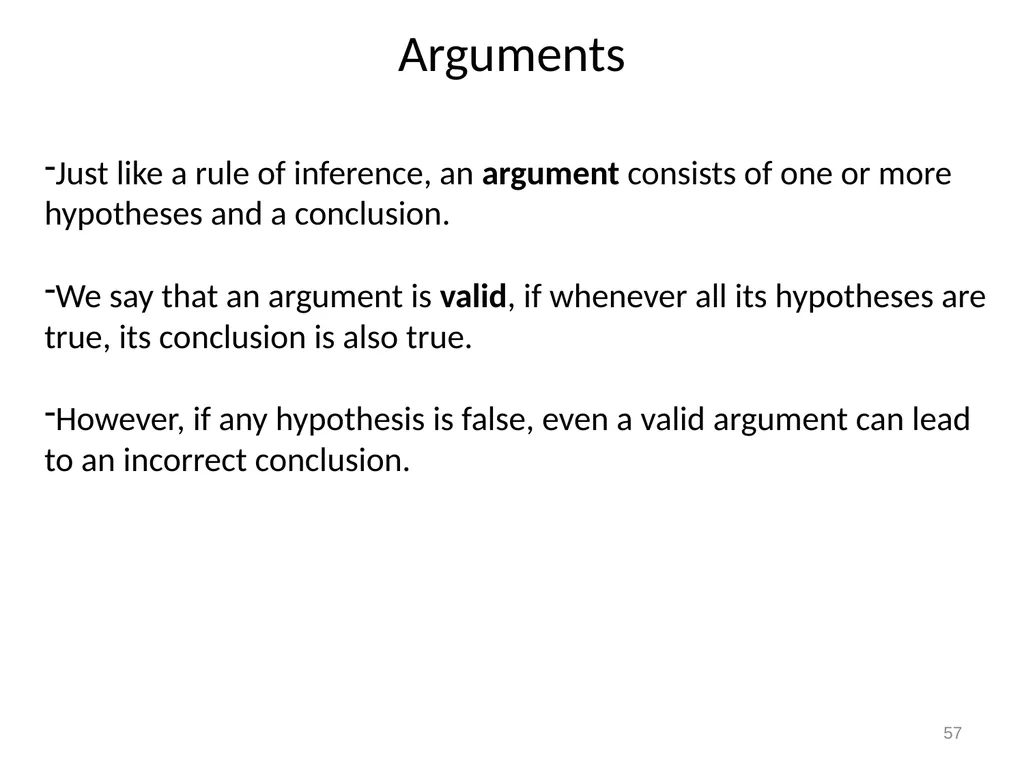
slide57. Arguments Just like a rule of inference, an argument consists of one or more hypotheses and a conclusion.

We say that an argument is valid, if whenever all its hypotheses are true, its conclusion is also true.

However, if any hypothesis is false, even a valid argument can lead to an incorrect conclusion. 57<br>
slide58. Predicate Calculus Predicate calculus
Inference theory of predicate calculus
Recurrence relations<br>
slide59. Predicate calculus
Predicates
Statement function
Variables
Quantifiers
Predicate formulas
Free and Bound variables
Universe of Discourse<br>
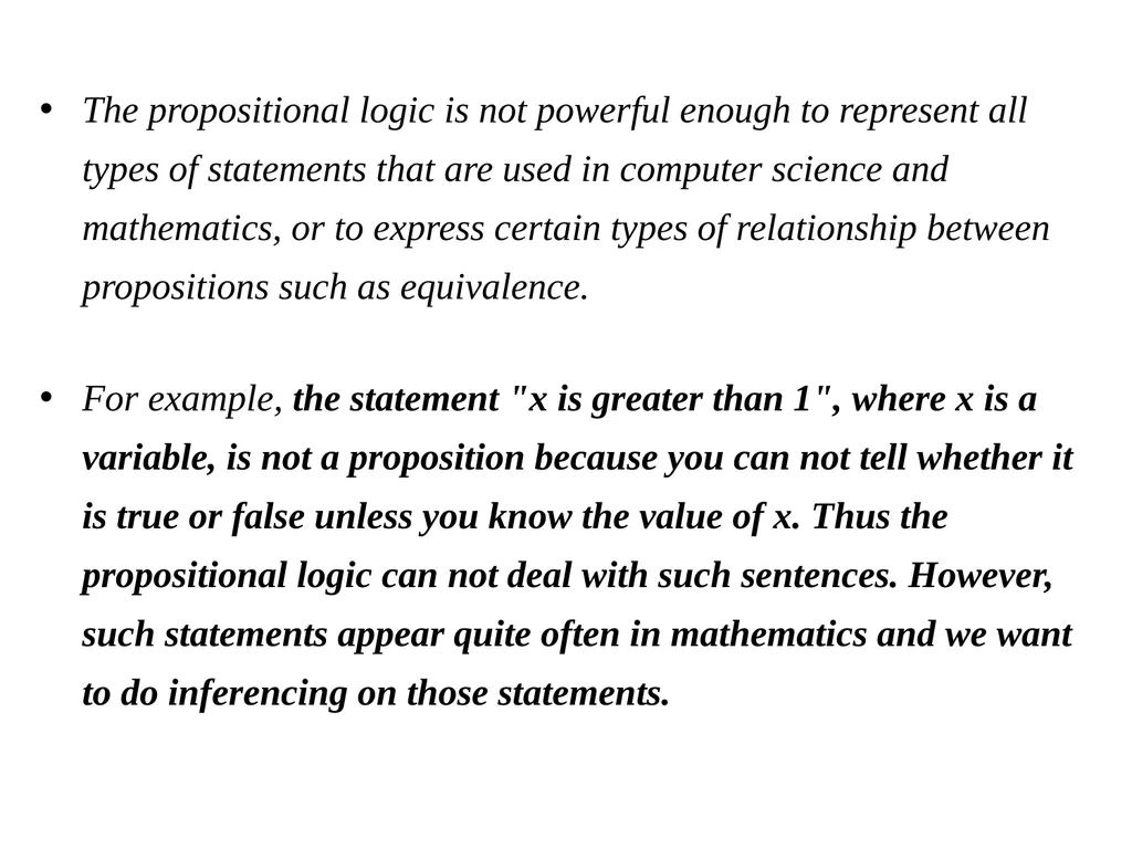
slide60. The propositional logic is not powerful enough to represent all types of statements that are used in computer science and mathematics, or to express certain types of relationship between propositions such as equivalence. 
For example, the statement "x is greater than 1", where x is a variable, is not a proposition because you can not tell whether it is true or false unless you know the value of x. Thus the propositional logic can not deal with such sentences. However, such statements appear quite often in mathematics and we want to do inferencing on those statements.<br>
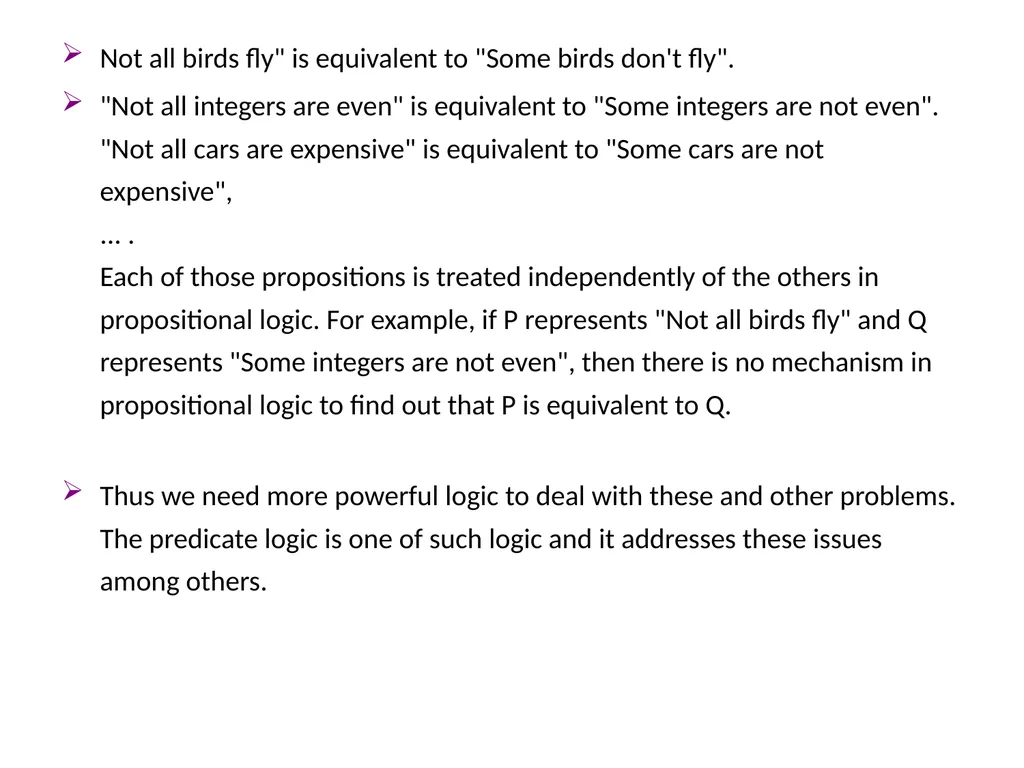
slide61. Not all birds fly" is equivalent to "Some birds don't fly".
"Not all integers are even" is equivalent to "Some integers are not even". "Not all cars are expensive" is equivalent to "Some cars are not expensive", ... . Each of those propositions is treated independently of the others in propositional logic. For example, if P represents "Not all birds fly" and Q represents "Some integers are not even", then there is no mechanism in propositional logic to find out that P is equivalent to Q. 
Thus we need more powerful logic to deal with these and other problems. The predicate logic is one of such logic and it addresses these issues among others.<br>
slide62. A predicate is a verb phrase template that describes a property of objects, or a relationship among objects represented by the variables.
The logic based upon the analysis of predicates in any statement is called predicate logic Predicates<br>
slide63. John is a bachelor.
Smith is a bachelor.
 the part “is a bachelor” is called a predicate.

All human beings are mortal.
John is a human being.
Therefore, John is a mortal.<br>
slide64. Symbolize a predicate by a capital letter and names of individuals or objects in general by small letters.
Every predicate describes about one or more objects.
Therefore a statement could be written symbolically in terms of the predicate letter followed by the name or names of the objects to which the predicate is applied.<br>
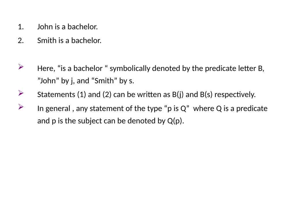
slide65. John is a bachelor.
Smith is a bachelor.

Here, “is a bachelor “ symbolically denoted by the predicate letter B, ”John” by j, and “Smith” by s.
Statements (1) and (2) can be written as B(j) and B(s) respectively.
In general , any statement of the type “p is Q” where Q is a predicate and p is the subject can be denoted by Q(p).<br>
slide66. A statement which is expressed by using a predicate letter must have at least one name of an object associated with the predicate.
A predicate requiring m(m>0) names is called an m-place predicate.
Example:
B in (1) and (2) is a 1-place predicate.
When m=0 , then we shall call a statement a 0-place predicate because no names are associated with a statement.<br>
slide67. This painting is red. R(p)
B(j)  R(p).
B(j)  R(p).
~R(p).

Statements involving the names of two objects
4. Jack is taller than Jill.
5. Canada is to the north of the United states.

Note: the order in which the names appear in the statement as well as in the predicate is important.<br>
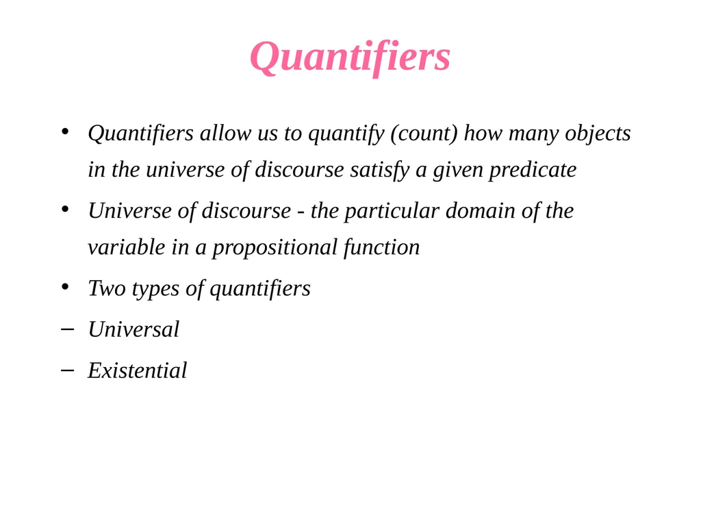
slide68. Quantifiers Quantifiers allow us to quantify (count) how many objects in the universe of discourse satisfy a given predicate
Universe of discourse - the particular domain of the variable in a propositional function
Two types of quantifiers
Universal
Existential<br>
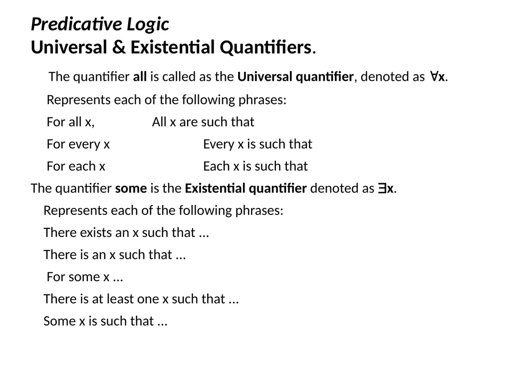
slide69. Predicative Logic
Universal & Existential Quantifiers.
The quantifier all is called as the Universal quantifier, denoted as x.
Represents each of the following phrases:
For all x, All x are such that
For every x Every x is such that
For each x Each x is such that
The quantifier some is the Existential quantifier denoted as x.
Represents each of the following phrases:
There exists an x such that ...
There is an x such that ...
For some x ...
There is at least one x such that ...
Some x is such that ...<br>
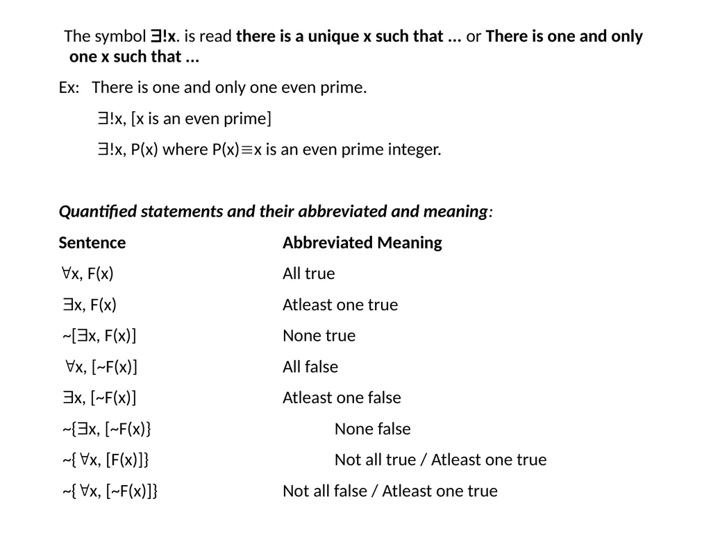
slide70. The symbol !x. is read there is a unique x such that ... or There is one and only one x such that ...
Ex: There is one and only one even prime.
!x, [x is an even prime]
!x, P(x) where P(x)x is an even prime integer.

Quantified statements and their abbreviated and meaning:
Sentence Abbreviated Meaning
x, F(x) All true
x, F(x) Atleast one true
~[x, F(x)] None true
x, [~F(x)] All false
x, [~F(x)] Atleast one false
~{x, [~F(x)} None false
~{x, [F(x)]} Not all true / Atleast one true
~{x, [~F(x)]} Not all false / Atleast one true<br>
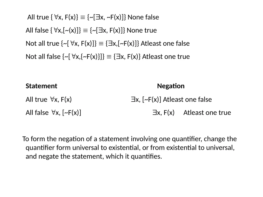
slide71. All true {x, F(x)}  {~[x, ~F(x)]} None false
All false {x,[~(x)]}  {~[x, F(x)]} None true
Not all true {~[x, F(x)]}  {x,[~F(x)]} Atleast one false
Not all false {~[x,{~F(x)}]}  {x, F(x)} Atleast one true

Statement Negation
All true x, F(x) x, [~F(x)] Atleast one false
All false x, [~F(x)] x, F(x) Atleast one true

To form the negation of a statement involving one quantifier, change the quantifier form universal to existential, or from existential to universal, and negate the statement, which it quantifies.<br>
slide72. Quantified Propositions:
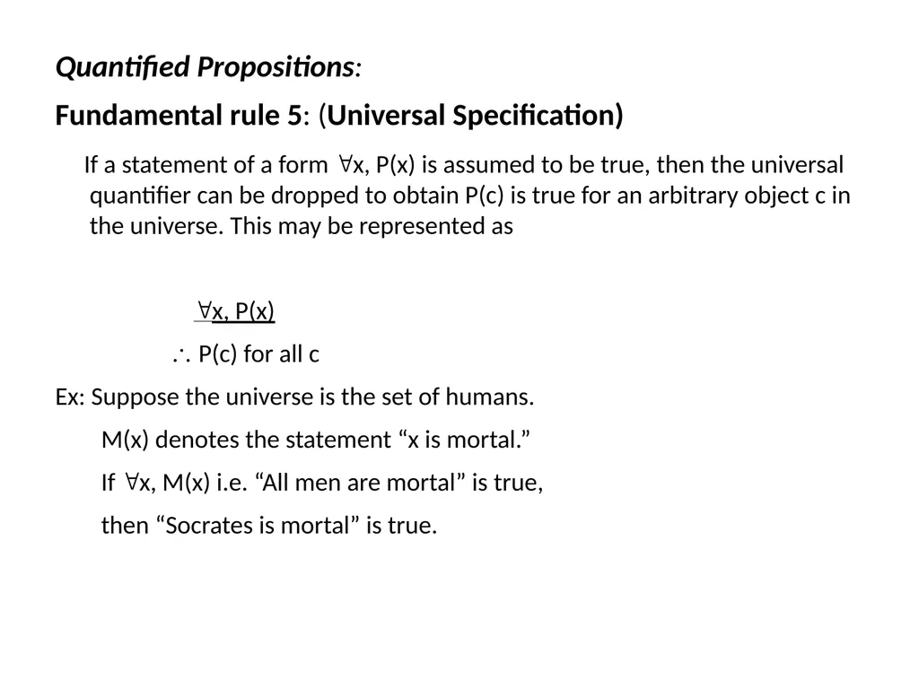
Fundamental rule 5: (Universal Specification)
If a statement of a form x, P(x) is assumed to be true, then the universal quantifier can be dropped to obtain P(c) is true for an arbitrary object c in the universe. This may be represented as

x, P(x)
 P(c) for all c
Ex: Suppose the universe is the set of humans.
M(x) denotes the statement “x is mortal.”
If x, M(x) i.e. “All men are mortal” is true,
then “Socrates is mortal” is true.<br>
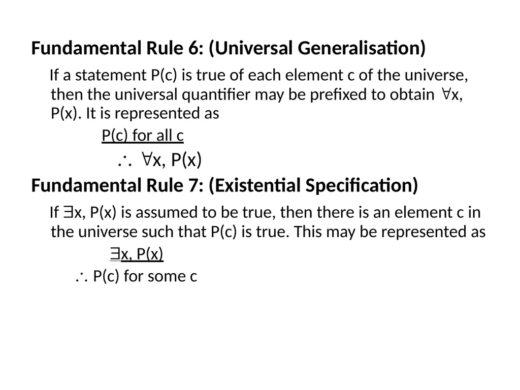
slide73. Fundamental Rule 6: (Universal Generalisation)
If a statement P(c) is true of each element c of the universe, then the universal quantifier may be prefixed to obtain x, P(x). It is represented as
P(c) for all c
 x, P(x)
Fundamental Rule 7: (Existential Specification)
If x, P(x) is assumed to be true, then there is an element c in the universe such that P(c) is true. This may be represented as
x, P(x)
 P(c) for some c<br>
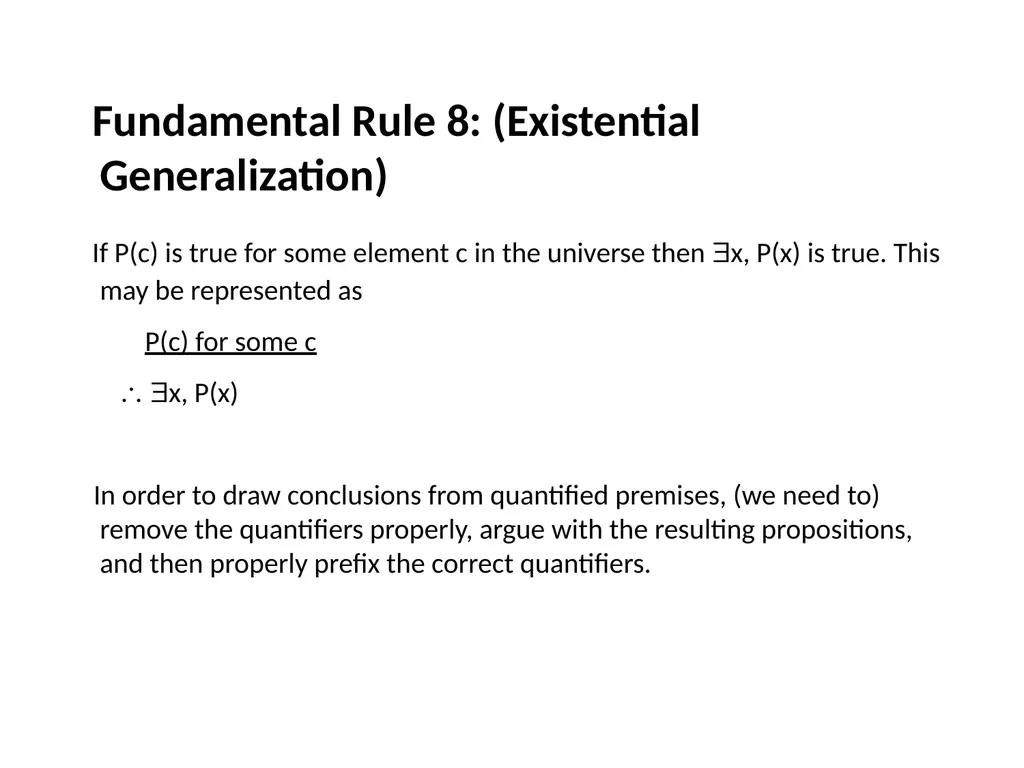
slide74. Fundamental Rule 8: (Existential Generalization)
If P(c) is true for some element c in the universe then x, P(x) is true. This may be represented as
P(c) for some c
 x, P(x)

In order to draw conclusions from quantified premises, (we need to) remove the quantifiers properly, argue with the resulting propositions, and then properly prefix the correct quantifiers.<br>
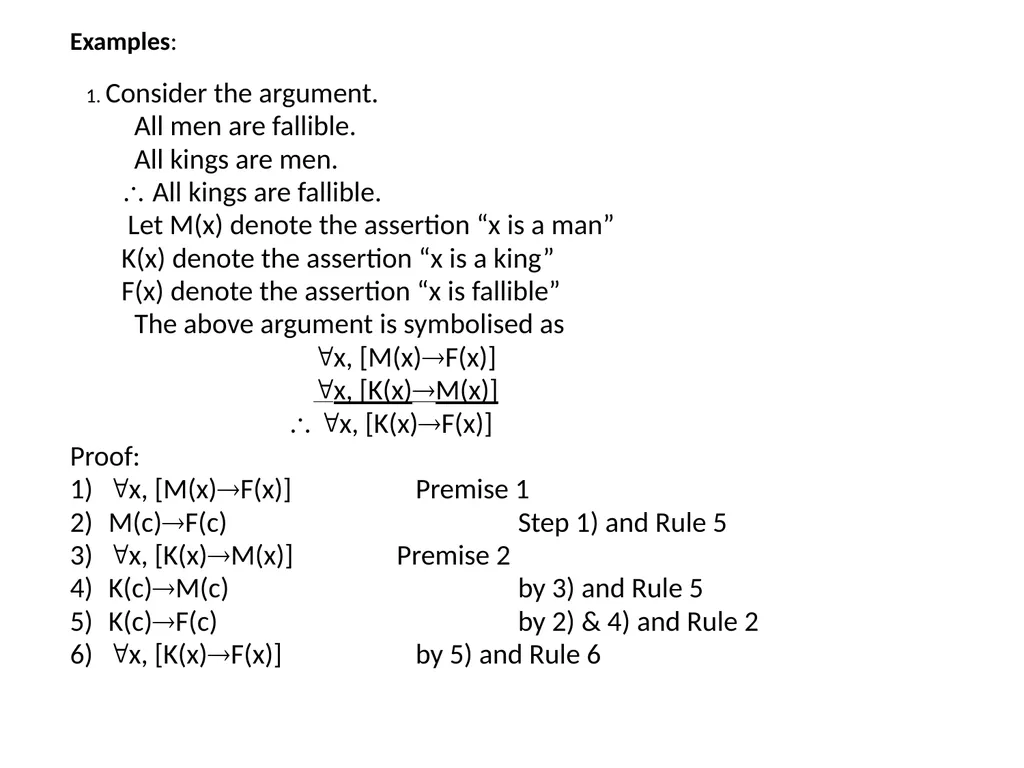
slide75. Examples:

1. Consider the argument.
All men are fallible.
All kings are men.
 All kings are fallible.
Let M(x) denote the assertion “x is a man”
K(x) denote the assertion “x is a king”
F(x) denote the assertion “x is fallible”
The above argument is symbolised as
x, [M(x)F(x)]
x, [K(x)M(x)]
 x, [K(x)F(x)]
Proof:
1) x, [M(x)F(x)] Premise 1
2) M(c)F(c) Step 1) and Rule 5
3) x, [K(x)M(x)] Premise 2
4) K(c)M(c) by 3) and Rule 5
5) K(c)F(c) by 2) & 4) and Rule 2
6) x, [K(x)F(x)] by 5) and Rule 6<br>
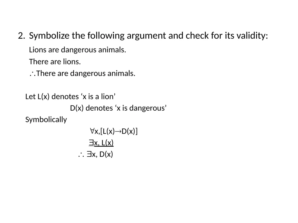
slide76. 2. Symbolize the following argument and check for its validity:
Lions are dangerous animals.
There are lions.
There are dangerous animals.

Let L(x) denotes ‘x is a lion’
D(x) denotes ‘x is dangerous’
Symbolically
x,[L(x)D(x)]
x, L(x)
 x, D(x)<br>
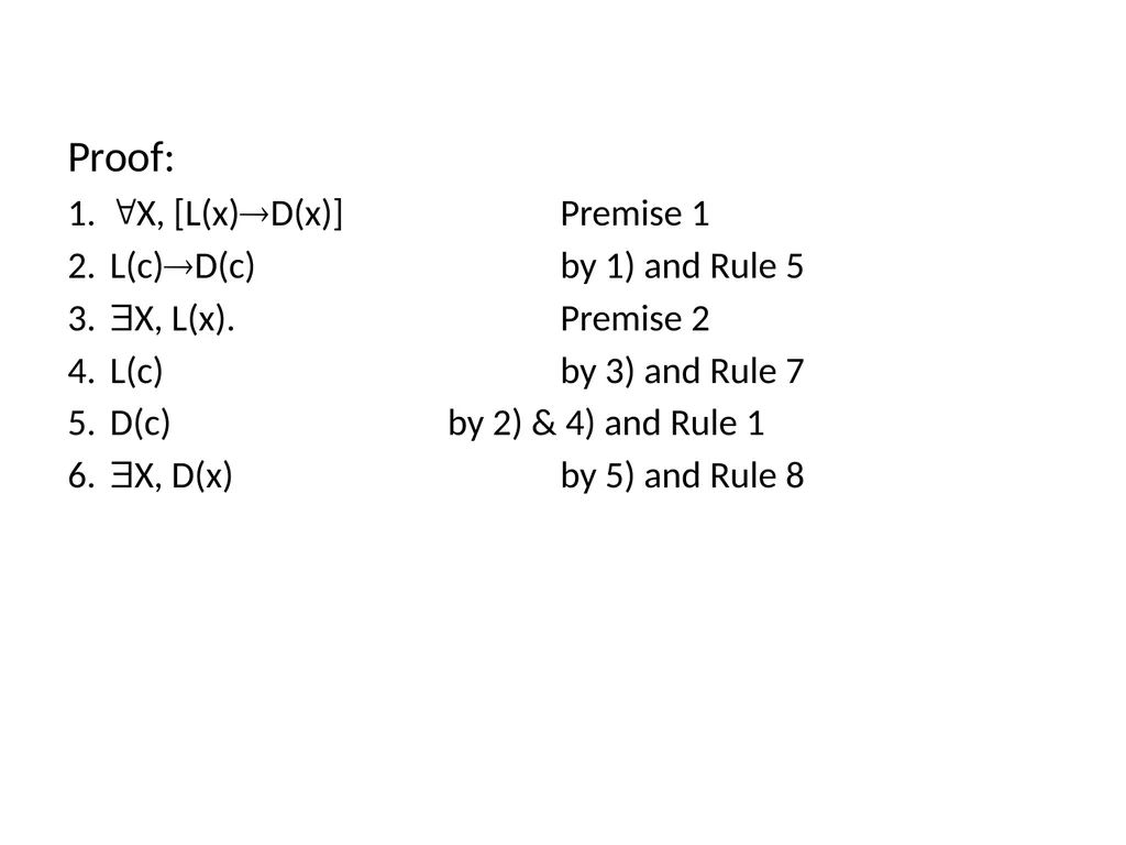
slide77. Proof:
1. X, [L(x)D(x)] Premise 1
2. L(c)D(c) by 1) and Rule 5
3. X, L(x). Premise 2
4. L(c) by 3) and Rule 7
5. D(c) by 2) & 4) and Rule 1
6. X, D(x) by 5) and Rule 8<br>
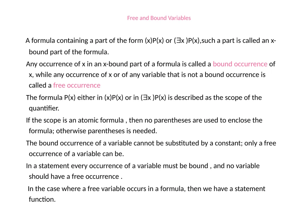
slide78. Free and Bound Variables A formula containing a part of the form (x)P(x) or (x )P(x),such a part is called an x-bound part of the formula.
Any occurrence of x in an x-bound part of a formula is called a bound occurrence of x, while any occurrence of x or of any variable that is not a bound occurrence is called a free occurrence
The formula P(x) either in (x)P(x) or in (x )P(x) is described as the scope of the quantifier.
If the scope is an atomic formula , then no parentheses are used to enclose the formula; otherwise parentheses is needed.
The bound occurrence of a variable cannot be substituted by a constant; only a free occurrence of a variable can be.
In a statement every occurrence of a variable must be bound , and no variable should have a free occurrence .
In the case where a free variable occurs in a formula, then we have a statement function.<br>