Dynamic Programming CSE 2320 – Algorithms and Data

slide1. Dynamic Programming CSE 2320 – Algorithms and Data Structures
University of Texas at Arlington

Alexandra Stefan
(Includes images, formulas and examples from CLRS, Dr. Bob Weems, wikipedia) 1 4/21/2020<br>
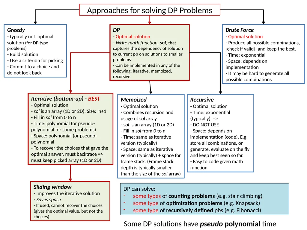
slide2. Approaches for solving DP Problems Greedy
- typically not optimal solution (for DP-type problems)
- Build solution
- Use a criterion for picking
- Commit to a choice and do not look back Brute Force
- Optimal solution
- Produce all possible combinations, [check if valid], and keep the best.
- Time: exponential
- Space: depends on implementation
- It may be hard to generate all possible combinations DP
- Optimal solution
- Write math function, sol, that captures the dependency of solution to current pb on solutions to smaller problems
- Can be implemented in any of the following: iterative, memoized, recursive Iterative (bottom-up) - BEST
- Optimal solution
- sol is an array (1D or 2D). Size: n+1
- Fill in sol from 0 to n
- Time: polynomial (or pseudo-polynomial for some problems)
- Space: polynomial (or pseudo-polynomial
- To recover the choices that gave the optimal answer, must backtrace => must keep picked array (1D or 2D). Sliding window
- Improves the iterative solution
- Saves space
- If used, cannot recover the choices (gives the optimal value, but not the choices) Memoized
- Optimal solution
- Combines recursion and usage of sol array.
- sol is an array (1D or 2D)
- Fill in sol from 0 to n
- Time: same as iterative version (typically)
- Space: same as iterative version (typically) + space for frame stack. (Frame stack depth is typically smaller than the size of the sol array) Recursive
- Optimal solution
- Time: exponential (typically) =>
- DO NOT USE
- Space: depends on implementation (code). E.g. store all combinations, or generate, evaluate on the fly and keep best seen so far.
- Easy to code given math function DP can solve:
some types of counting problems (e.g. stair climbing)
some type of optimization problems (e.g. Knapsack)
some type of recursively defined pbs (e.g. Fibonacci) Some DP solutions have pseudo polynomial time<br>
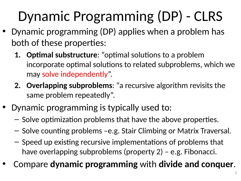
slide3. Dynamic Programming (DP) - CLRS Dynamic programming (DP) applies when a problem has both of these properties:
Optimal substructure: “optimal solutions to a problem incorporate optimal solutions to related subproblems, which we may solve independently”.
Overlapping subproblems: “a recursive algorithm revisits the same problem repeatedly”.
Dynamic programming is typically used to:
Solve optimization problems that have the above properties.
Solve counting problems –e.g. Stair Climbing or Matrix Traversal.
Speed up existing recursive implementations of problems that have overlapping subproblems (property 2) – e.g. Fibonacci.
Compare dynamic programming with divide and conquer. 3<br>
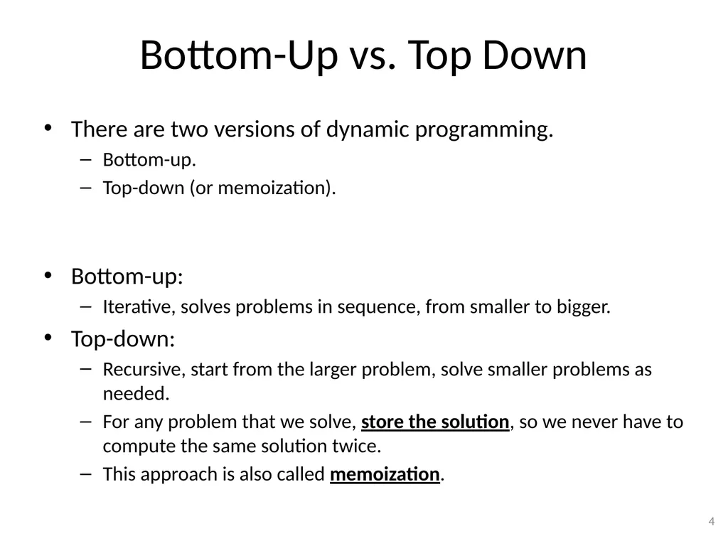
slide4. Bottom-Up vs. Top Down There are two versions of dynamic programming.
Bottom-up.
Top-down (or memoization).

Bottom-up:
Iterative, solves problems in sequence, from smaller to bigger.
Top-down:
Recursive, start from the larger problem, solve smaller problems as needed.
For any problem that we solve, store the solution, so we never have to compute the same solution twice.
This approach is also called memoization. 4<br>
slide5. Top-Down Dynamic Programming( Memoization ) Maintain an array/table where solutions to problems can be saved.
To solve a problem P:
See if the solution has already been stored in the array.
If yes, return the solution.
Else:
Issue recursive calls to solve whatever smaller problems we need to solve.
Using those solutions obtain the solution to problem P.
Store the solution in the solutions array.
Return the solution. 5<br>
slide6. Bottom-Up Dynamic Programming Requirements for using dynamic programming:
The answer to our problem, P, can be easily obtained from answers to smaller problems.
We can order problems in a sequence (P0, P1, P2, ..., PK) of reasonable size, so that:
Pk is our original problem P.
The initial problems, P0 and possibly P1, P2, ..., PR up to some R, are easy to solve (they are base cases).
For i > R, each Pi can be easily solved using solutions to P0, ..., Pi-1.
If these requirements are met, we solve problem P as follows:
Create the sequence of problems P0, P1, P2, ..., PK, such that Pk = P.
For i = 0 to K, solve PK.
Return solution for PK. 6<br>
slide7. Steps (Dr. Weems) Identify problem input
Identify the cost/gain function (name it, describe it)
Give the math formula for the cost function for all cases: base cases and general case
Order the problems & solve them
Recover the choices that gave the optimal value

Other
Brute force solution
Recursive solution (most likely exponential and inneficient)
Memoized solution 7<br>
slide8. Fibonacci Numbers 8<br>
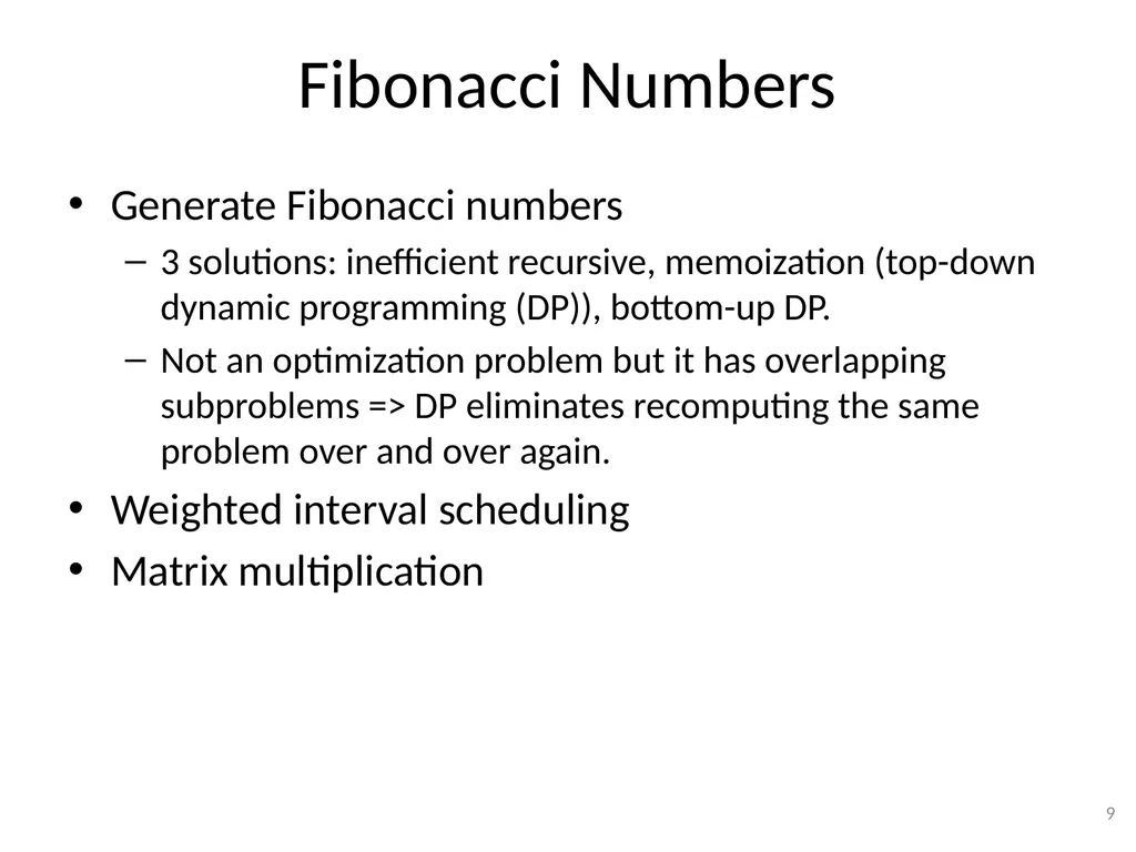
slide9. Fibonacci Numbers Generate Fibonacci numbers
3 solutions: inefficient recursive, memoization (top-down dynamic programming (DP)), bottom-up DP.
Not an optimization problem but it has overlapping subproblems => DP eliminates recomputing the same problem over and over again.
Weighted interval scheduling
Matrix multiplication 9<br>
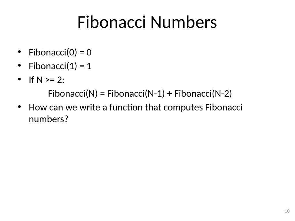
slide10. Fibonacci Numbers Fibonacci(0) = 0
Fibonacci(1) = 1
If N >= 2:
Fibonacci(N) = Fibonacci(N-1) + Fibonacci(N-2)
How can we write a function that computes Fibonacci numbers? 10<br>
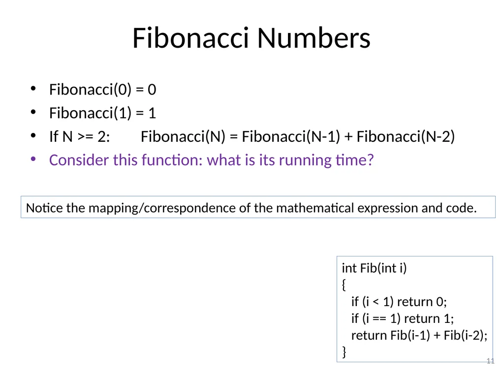
slide11. Fibonacci Numbers Fibonacci(0) = 0
Fibonacci(1) = 1
If N >= 2: Fibonacci(N) = Fibonacci(N-1) + Fibonacci(N-2)
Consider this function: what is its running time? 11 int Fib(int i)
{
if (i < 1) return 0;
if (i == 1) return 1;
return Fib(i-1) + Fib(i-2);
} Notice the mapping/correspondence of the mathematical expression and code.<br>
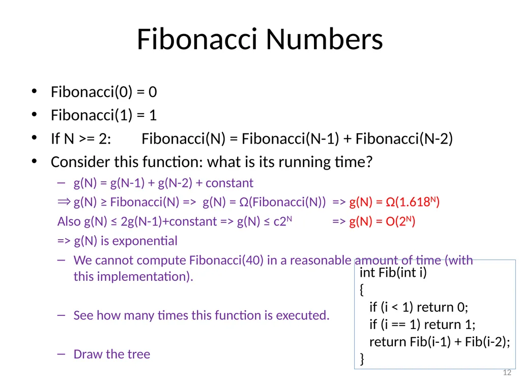
slide12. Fibonacci Numbers Fibonacci(0) = 0
Fibonacci(1) = 1
If N >= 2: Fibonacci(N) = Fibonacci(N-1) + Fibonacci(N-2)
Consider this function: what is its running time?
g(N) = g(N-1) + g(N-2) + constant
g(N) ≥ Fibonacci(N) => g(N) = Ω(Fibonacci(N)) => g(N) = Ω(1.618N)
Also g(N) ≤ 2g(N-1)+constant => g(N) ≤ c2N => g(N) = O(2N)
=> g(N) is exponential
We cannot compute Fibonacci(40) in a reasonable amount of time (with this implementation).

See how many times this function is executed.

Draw the tree 12 int Fib(int i)
{
if (i < 1) return 0;
if (i == 1) return 1;
return Fib(i-1) + Fib(i-2);
}<br>
slide13. Fibonacci Numbers Fibonacci(0) = 0
Fibonacci(1) = 1
If N >= 2: Fibonacci(N) = Fibonacci(N-1) + Fibonacci(N-2)
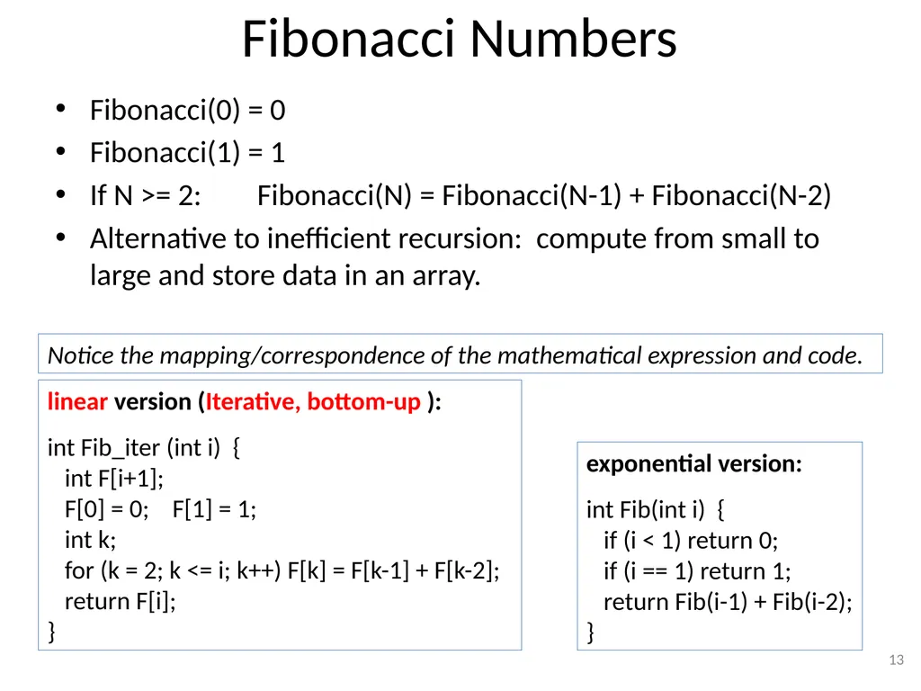
Alternative to inefficient recursion: compute from small to large and store data in an array. 13 exponential version:

int Fib(int i) {
if (i < 1) return 0;
if (i == 1) return 1;
return Fib(i-1) + Fib(i-2);
} linear version (Iterative, bottom-up ):

int Fib_iter (int i) {
int F[i+1];
F[0] = 0; F[1] = 1;
int k;
for (k = 2; k <= i; k++) F[k] = F[k-1] + F[k-2];
return F[i];
} Notice the mapping/correspondence of the mathematical expression and code.<br>
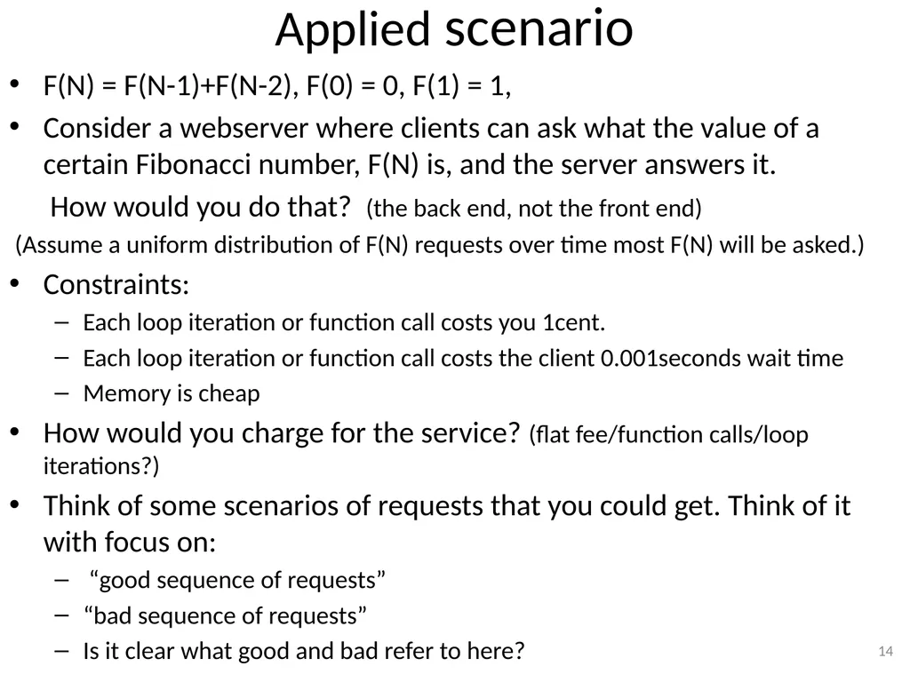
slide14. Applied scenario F(N) = F(N-1)+F(N-2), F(0) = 0, F(1) = 1,
Consider a webserver where clients can ask what the value of a certain Fibonacci number, F(N) is, and the server answers it.
How would you do that? (the back end, not the front end)
(Assume a uniform distribution of F(N) requests over time most F(N) will be asked.)
Constraints:
Each loop iteration or function call costs you 1cent.
Each loop iteration or function call costs the client 0.001seconds wait time
Memory is cheap
How would you charge for the service? (flat fee/function calls/loop iterations?)
Think of some scenarios of requests that you could get. Think of it with focus on:
“good sequence of requests”
“bad sequence of requests”
Is it clear what good and bad refer to here? 14<br>
slide15. Fibonacci Numbers Fibonacci(0) = 0 , Fibonacci(1) = 1
If N >= 2: Fibonacci(N) = Fibonacci(N-1) + Fibonacci(N-2)
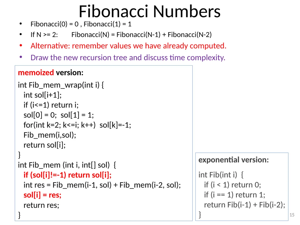
Alternative: remember values we have already computed.
Draw the new recursion tree and discuss time complexity. 15 exponential version:

int Fib(int i) {
if (i < 1) return 0;
if (i == 1) return 1;
return Fib(i-1) + Fib(i-2);
} memoized version:

int Fib_mem_wrap(int i) {
int sol[i+1];
if (i<=1) return i;
sol[0] = 0; sol[1] = 1;
for(int k=2; k<=i; k++) sol[k]=-1;
Fib_mem(i,sol);
return sol[i];
}
int Fib_mem (int i, int[] sol) {
if (sol[i]!=-1) return sol[i];
int res = Fib_mem(i-1, sol) + Fib_mem(i-2, sol);
sol[i] = res;
return res;
}<br>
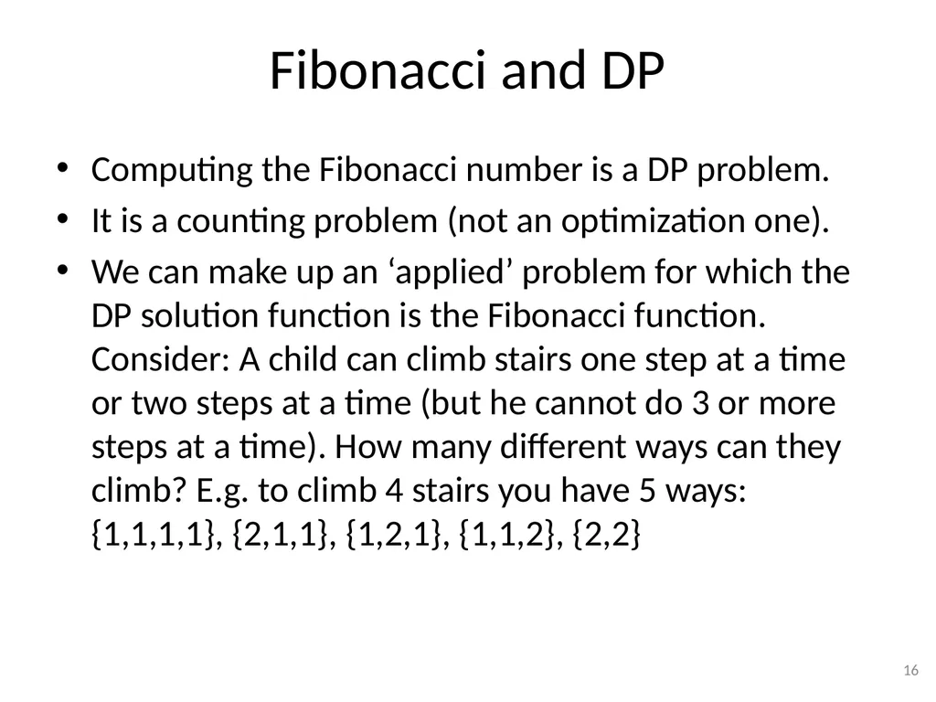
slide16. Fibonacci and DP Computing the Fibonacci number is a DP problem.
It is a counting problem (not an optimization one).
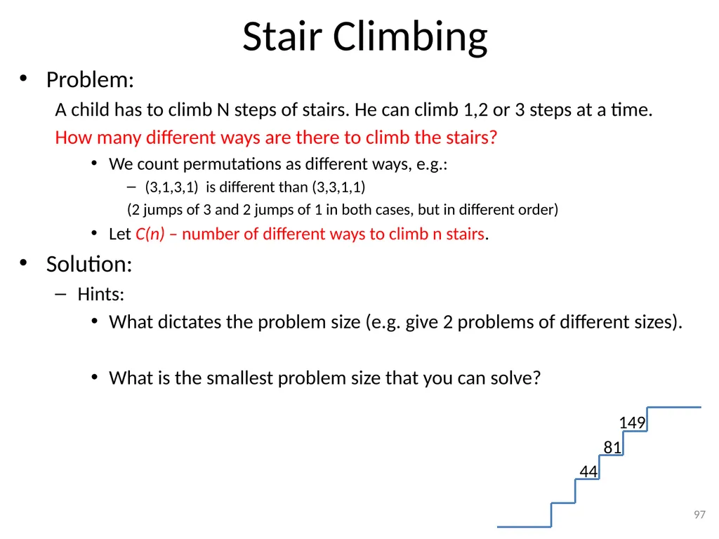
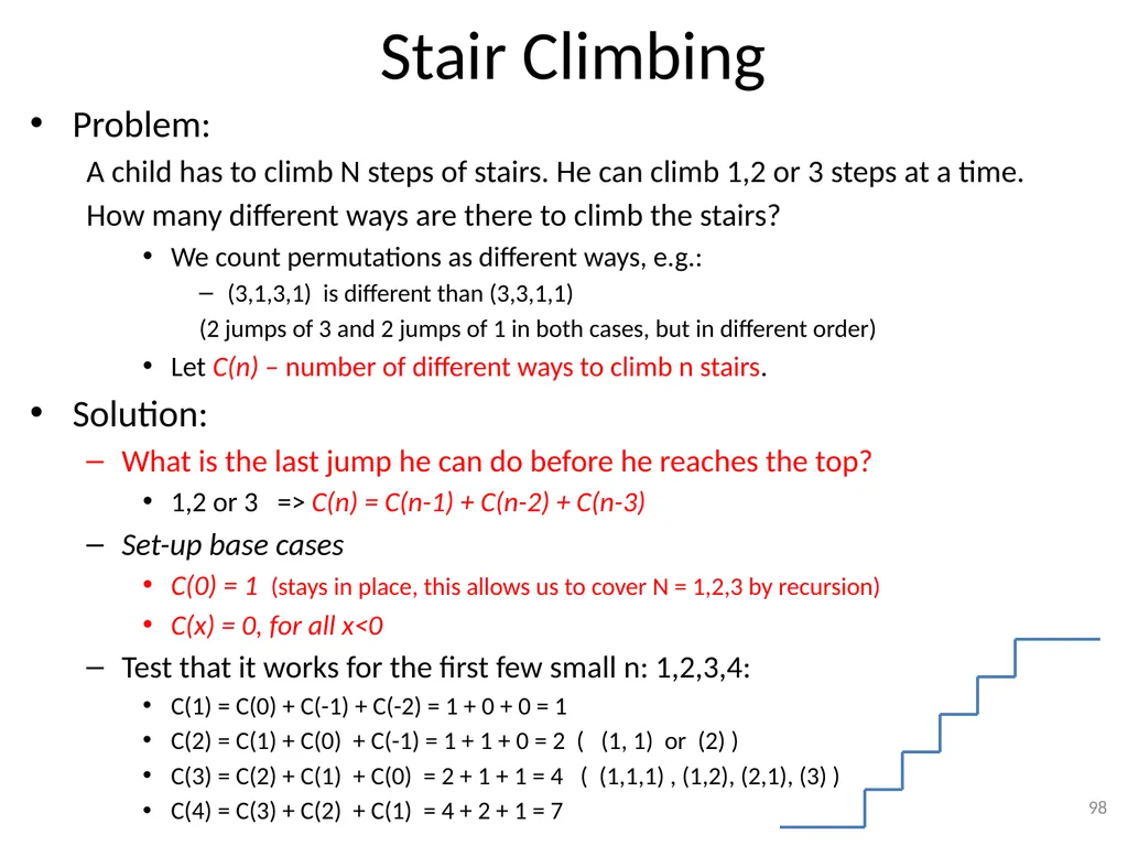
We can make up an ‘applied’ problem for which the DP solution function is the Fibonacci function. Consider: A child can climb stairs one step at a time or two steps at a time (but he cannot do 3 or more steps at a time). How many different ways can they climb? E.g. to climb 4 stairs you have 5 ways: {1,1,1,1}, {2,1,1}, {1,2,1}, {1,1,2}, {2,2} 16<br>
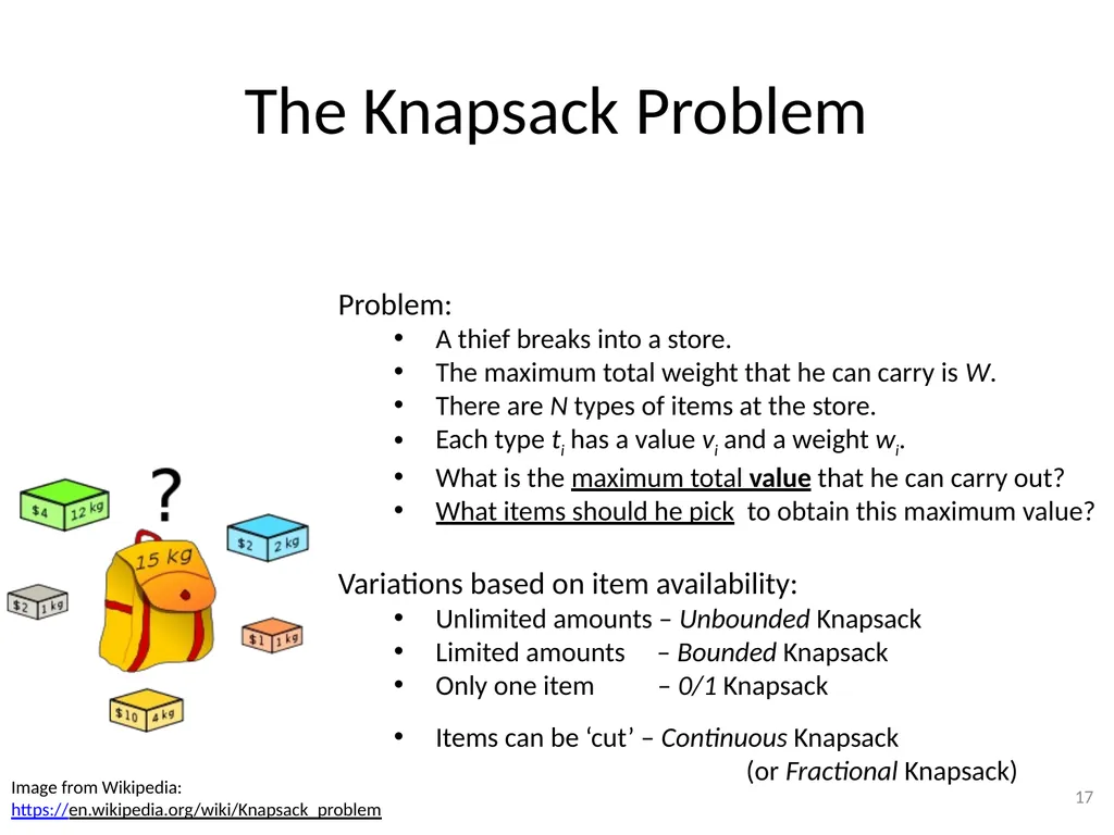
slide17. 17 The Knapsack Problem Image from Wikipedia:
https://en.wikipedia.org/wiki/Knapsack_problem Problem:
A thief breaks into a store.
The maximum total weight that he can carry is W.
There are N types of items at the store.
Each type ti has a value vi and a weight wi.
What is the maximum total value that he can carry out?
What items should he pick to obtain this maximum value?

Variations based on item availability:
Unlimited amounts – Unbounded Knapsack
Limited amounts – Bounded Knapsack
Only one item – 0/1 Knapsack

Items can be ‘cut’ – Continuous Knapsack (or Fractional Knapsack)<br>
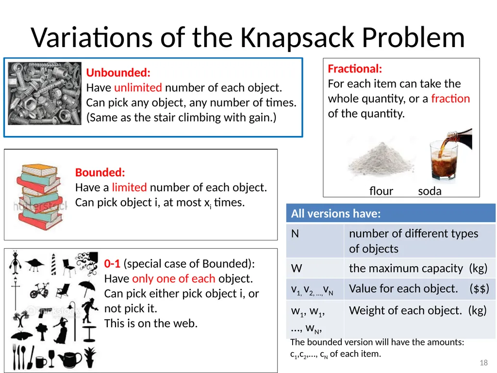
slide18. Variations of the Knapsack Problem 18 Fractional:
For each item can take the whole quantity, or a fraction of the quantity. flour soda Unbounded:
Have unlimited number of each object.
Can pick any object, any number of times.
(Same as the stair climbing with gain.) Bounded:
Have a limited number of each object.
Can pick object i, at most xi times. 0-1 (special case of Bounded):
Have only one of each object.
Can pick either pick object i, or not pick it.
This is on the web. The bounded version will have the amounts:
c1,c2,…, cN of each item.<br>
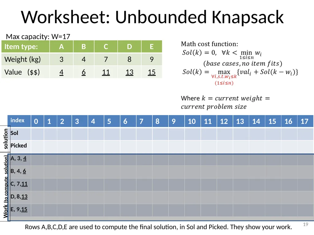
slide19. Worksheet: Unbounded Knapsack 19 Rows A,B,C,D,E are used to compute the final solution, in Sol and Picked. They show your work. Max capacity: W=17 solution Work (to compute solution)<br>
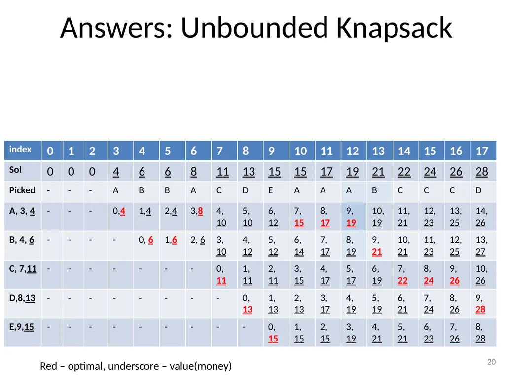
slide20. Answers: Unbounded Knapsack 20 Red – optimal, underscore – value(money)<br>
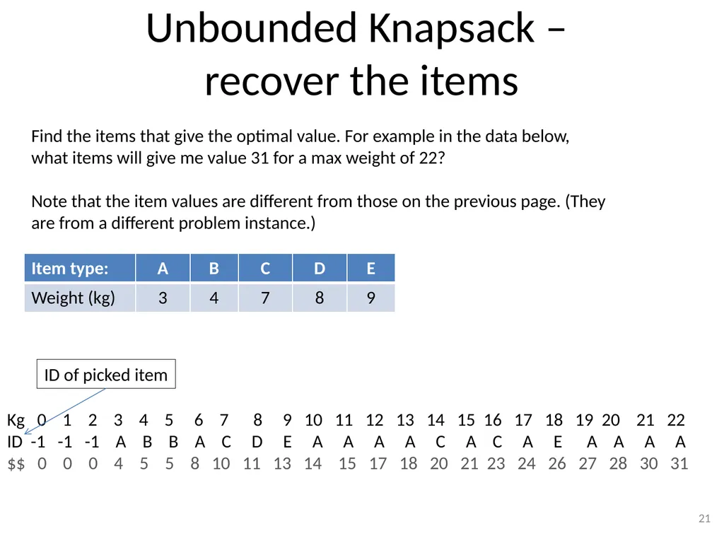
slide21. Unbounded Knapsack – recover the items 21 Kg 0 1 2 3 4 5 6 7 8 9 10 11 12 13 14 15 16 17 18 19 20 21 22
ID -1 -1 -1 A B B A C D E A A A A C A C A E A A A A
$$ 0 0 0 4 5 5 8 10 11 13 14 15 17 18 20 21 23 24 26 27 28 30 31 Find the items that give the optimal value. For example in the data below, what items will give me value 31 for a max weight of 22?

Note that the item values are different from those on the previous page. (They are from a different problem instance.) ID of picked item<br>
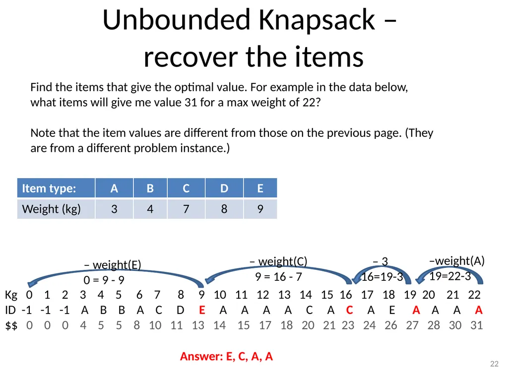
slide22. Unbounded Knapsack – recover the items 22 Kg 0 1 2 3 4 5 6 7 8 9 10 11 12 13 14 15 16 17 18 19 20 21 22
ID -1 -1 -1 A B B A C D E A A A A C A C A E A A A A
$$ 0 0 0 4 5 5 8 10 11 13 14 15 17 18 20 21 23 24 26 27 28 30 31 Find the items that give the optimal value. For example in the data below, what items will give me value 31 for a max weight of 22?

Note that the item values are different from those on the previous page. (They are from a different problem instance.) –weight(A)
19=22-3 – 3
16=19-3 – weight(C)
9 = 16 - 7 – weight(E)
0 = 9 - 9 Answer: E, C, A, A<br>
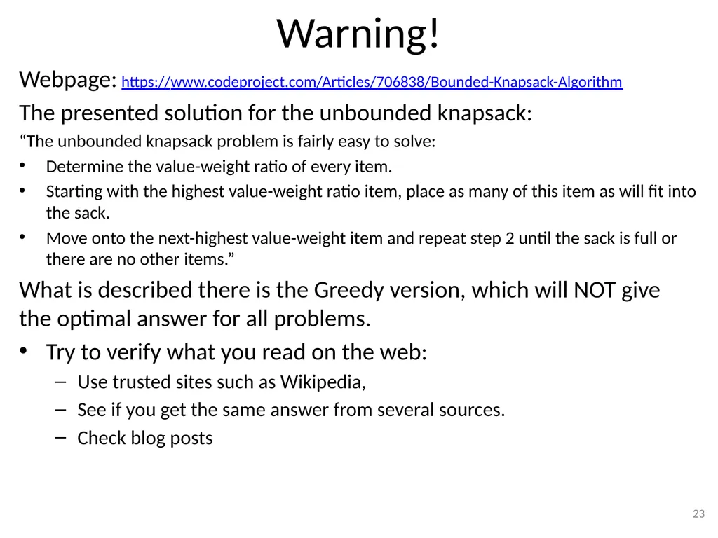
slide23. Warning! Webpage: https://www.codeproject.com/Articles/706838/Bounded-Knapsack-Algorithm
The presented solution for the unbounded knapsack:
“The unbounded knapsack problem is fairly easy to solve:
Determine the value-weight ratio of every item.
Starting with the highest value-weight ratio item, place as many of this item as will fit into the sack.
Move onto the next-highest value-weight item and repeat step 2 until the sack is full or there are no other items.”
What is described there is the Greedy version, which will NOT give the optimal answer for all problems.
Try to verify what you read on the web:
Use trusted sites such as Wikipedia,
See if you get the same answer from several sources.
Check blog posts 23<br>
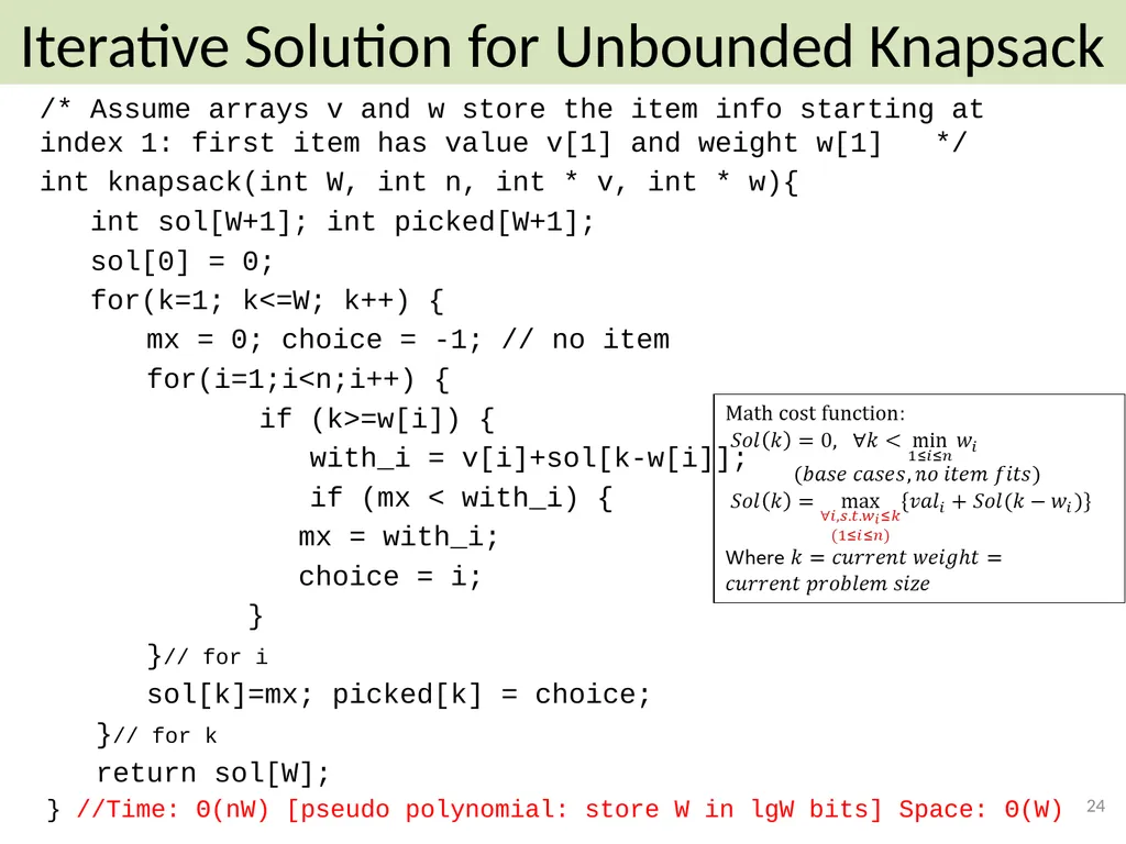
slide24. Iterative Solution for Unbounded Knapsack /* Assume arrays v and w store the item info starting at index 1: first item has value v[1] and weight w[1] */
int knapsack(int W, int n, int * v, int * w){
int sol[W+1]; int picked[W+1];
sol[0] = 0;
for(k=1; k<=W; k++) {
mx = 0; choice = -1; // no item
for(i=1;i<n;i++) {
if (k>=w[i]) {
with_i = v[i]+sol[k-w[i]];
if (mx < with_i) {
mx = with_i;
choice = i;
}
}// for i
sol[k]=mx; picked[k] = choice;
}// for k
return sol[W];
} //Time: Θ(nW) [pseudo polynomial: store W in lgW bits] Space: Θ(W) 24<br>
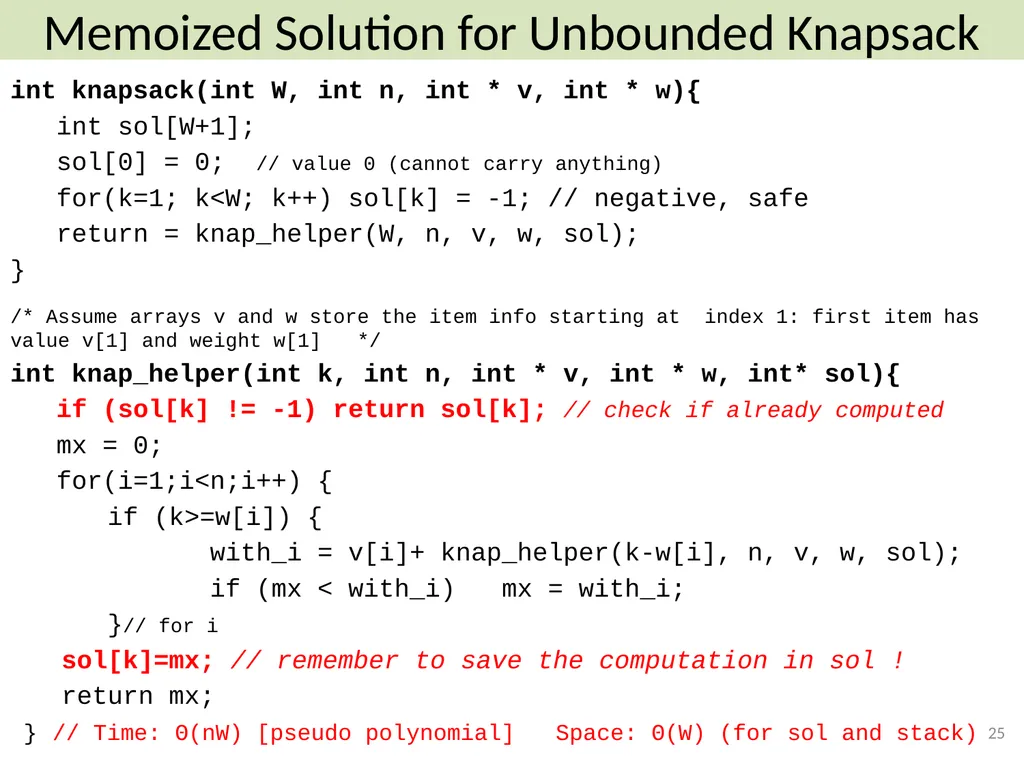
slide25. int knapsack(int W, int n, int * v, int * w){
int sol[W+1];
sol[0] = 0; // value 0 (cannot carry anything)
for(k=1; k<W; k++) sol[k] = -1; // negative, safe
return = knap_helper(W, n, v, w, sol);
}

/* Assume arrays v and w store the item info starting at index 1: first item has value v[1] and weight w[1] */
int knap_helper(int k, int n, int * v, int * w, int* sol){
if (sol[k] != -1) return sol[k]; // check if already computed
mx = 0;
for(i=1;i<n;i++) {
if (k>=w[i]) {
with_i = v[i]+ knap_helper(k-w[i], n, v, w, sol);
if (mx < with_i) mx = with_i;
}// for i
sol[k]=mx; // remember to save the computation in sol !
return mx;
} // Time: Θ(nW) [pseudo polynomial] Space: Θ(W) (for sol and stack) 25 Memoized Solution for Unbounded Knapsack<br>
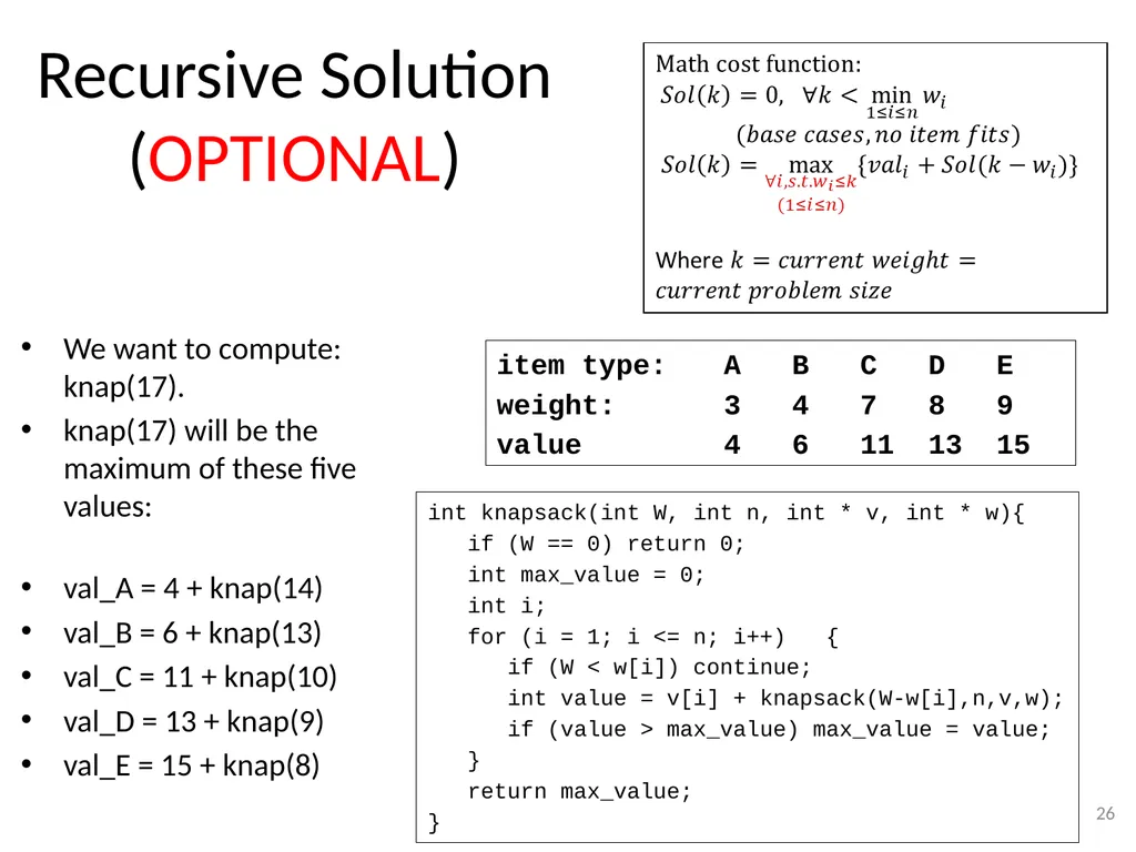
slide26. Recursive Solution (OPTIONAL) We want to compute: knap(17).
knap(17) will be the maximum of these five values:
val_A = 4 + knap(14)
val_B = 6 + knap(13)
val_C = 11 + knap(10)
val_D = 13 + knap(9)
val_E = 15 + knap(8) 26 item type: A B C D E
weight: 3 4 7 8 9
value 4 6 11 13 15 int knapsack(int W, int n, int * v, int * w){
if (W == 0) return 0;
int max_value = 0;
int i;
for (i = 1; i <= n; i++) {
if (W < w[i]) continue;
int value = v[i] + knapsack(W-w[i],n,v,w);
if (value > max_value) max_value = value;
}
return max_value;
}<br>
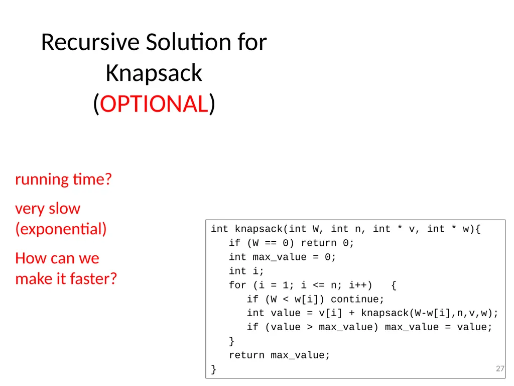
slide27. Recursive Solution for Knapsack(OPTIONAL) 27 running time?

very slow (exponential)

How can we make it faster? int knapsack(int W, int n, int * v, int * w){
if (W == 0) return 0;
int max_value = 0;
int i;
for (i = 1; i <= n; i++) {
if (W < w[i]) continue;
int value = v[i] + knapsack(W-w[i],n,v,w);
if (value > max_value) max_value = value;
}
return max_value;
}<br>
slide28. Draw the recursion tree(OPTIONAL) Inefficient recursion
Memoized version 28<br>
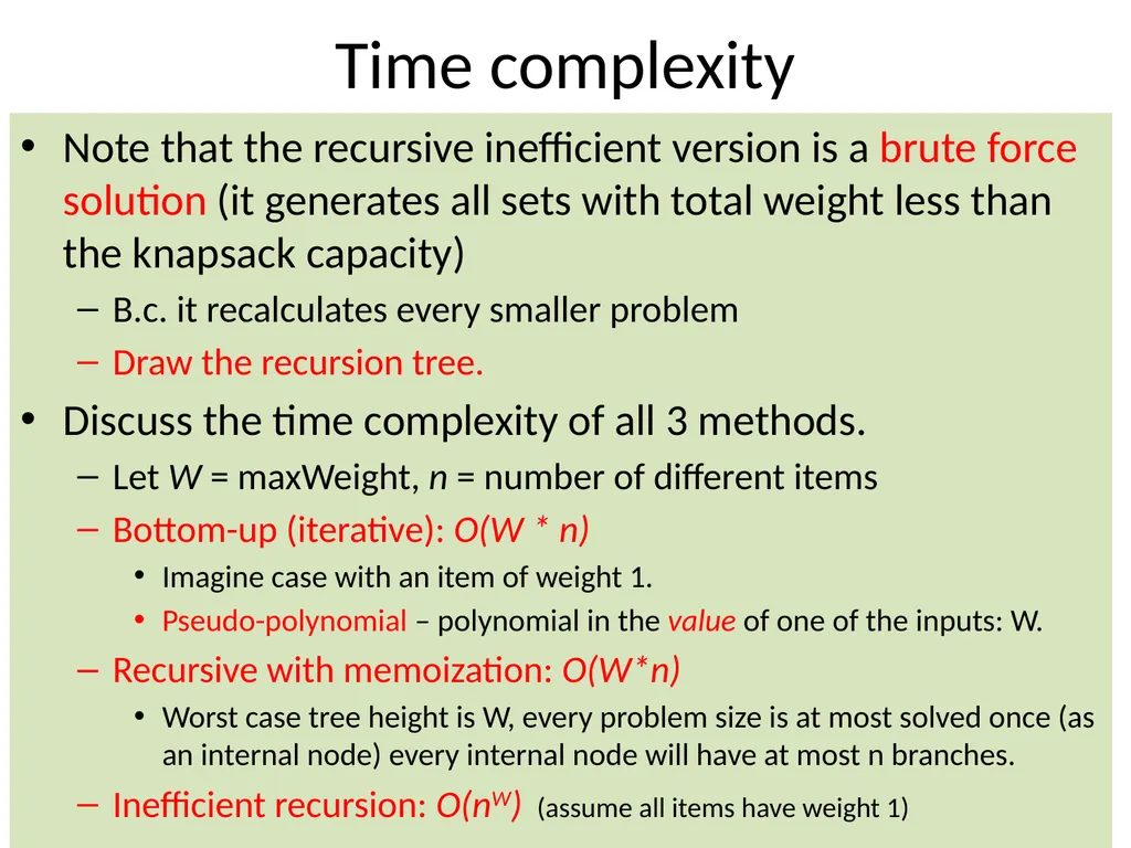
slide29. Time complexity Note that the recursive inefficient version is a brute force solution (it generates all sets with total weight less than the knapsack capacity)
B.c. it recalculates every smaller problem
Draw the recursion tree.
Discuss the time complexity of all 3 methods.
Let W = maxWeight, n = number of different items
Bottom-up (iterative): O(W * n)
Imagine case with an item of weight 1.
Pseudo-polynomial – polynomial in the value of one of the inputs: W.
Recursive with memoization: O(W*n)
Worst case tree height is W, every problem size is at most solved once (as an internal node) every internal node will have at most n branches.
Inefficient recursion: O(nW) (assume all items have weight 1) 29<br>
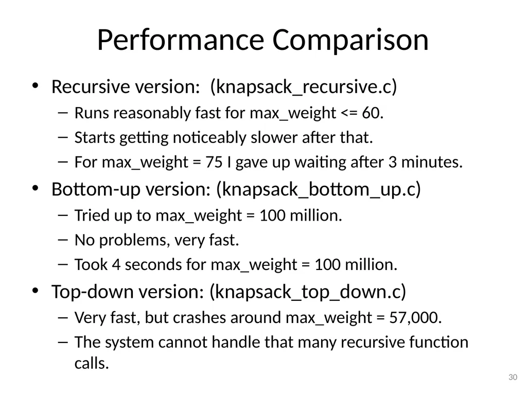
slide30. Performance Comparison Recursive version: (knapsack_recursive.c)
Runs reasonably fast for max_weight <= 60.
Starts getting noticeably slower after that.
For max_weight = 75 I gave up waiting after 3 minutes.
Bottom-up version: (knapsack_bottom_up.c)
Tried up to max_weight = 100 million.
No problems, very fast.
Took 4 seconds for max_weight = 100 million.
Top-down version: (knapsack_top_down.c)
Very fast, but crashes around max_weight = 57,000.
The system cannot handle that many recursive function calls. 30<br>
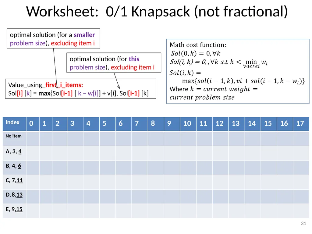
slide31. Worksheet: 0/1 Knapsack (not fractional) 31 Value_using_first_i_items:
Sol[i] [k] = max{Sol[i-1] [ k – w[i]] + v[i], Sol[i-1] [k] optimal solution (for a smaller problem size), excluding item i optimal solution (for this problem size), excluding item i<br>
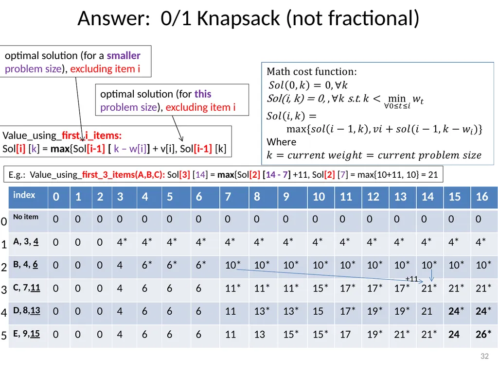
slide32. Answer: 0/1 Knapsack (not fractional) 32 Value_using_first_i_items:
Sol[i] [k] = max{Sol[i-1] [ k – w[i]] + v[i], Sol[i-1] [k] optimal solution (for a smaller problem size), excluding item i optimal solution (for this problem size), excluding item i E.g.: Value_using_first_3_items(A,B,C): Sol[3] [14] = max{Sol[2] [14 - 7] +11, Sol[2] [7] = max{10+11, 10} = 21 +11<br>
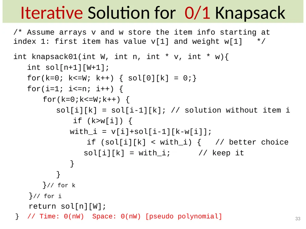
slide33. Iterative Solution for 0/1 Knapsack /* Assume arrays v and w store the item info starting at index 1: first item has value v[1] and weight w[1] */

int knapsack01(int W, int n, int * v, int * w){
int sol[n+1][W+1];
for(k=0; k<=W; k++) { sol[0][k] = 0;}
for(i=1; i<=n; i++) {
for(k=0;k<=W;k++) {
sol[i][k] = sol[i-1][k]; // solution without item i
if (k>w[i]) {
with_i = v[i]+sol[i-1][k-w[i]];
if (sol[i][k] < with_i) { // better choice
sol[i][k] = with_i; // keep it
}
}
}// for k
}// for i
return sol[n][W];
} // Time: Θ(nW) Space: Θ(nW) [pseudo polynomial] 33<br>
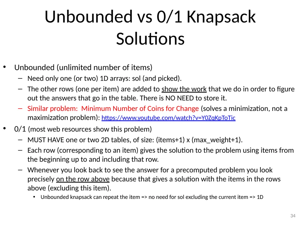
slide34. Unbounded vs 0/1 KnapsackSolutions Unbounded (unlimited number of items)
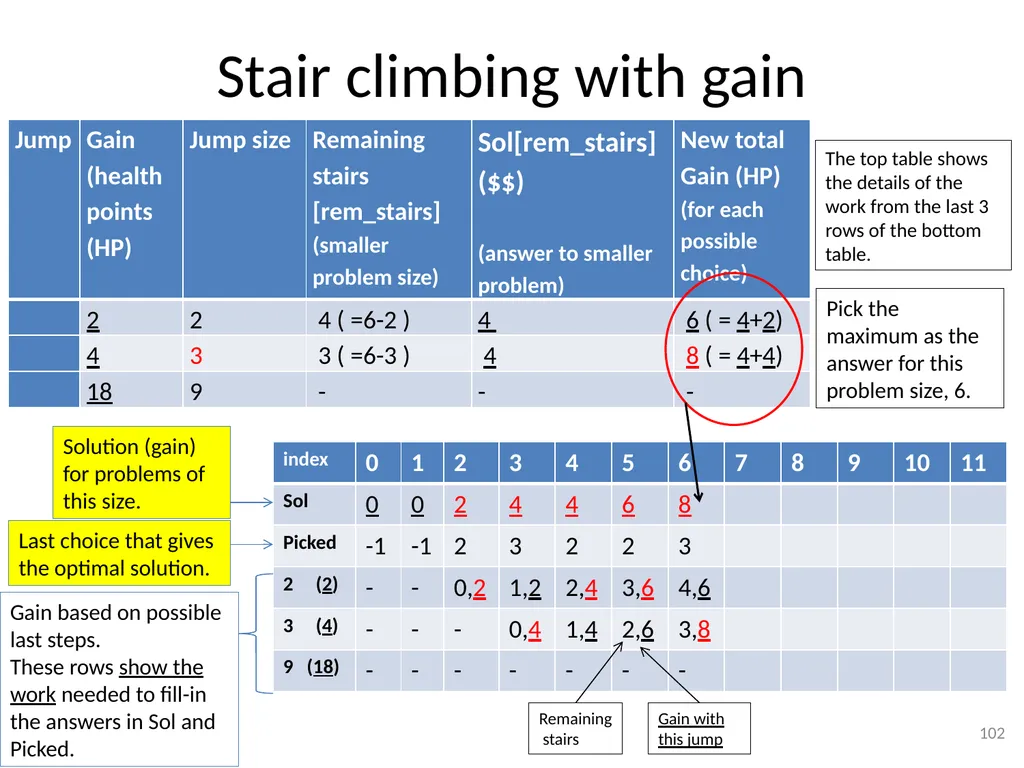
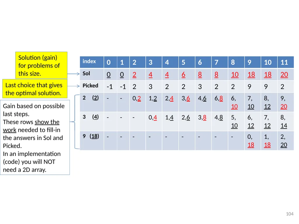
Need only one (or two) 1D arrays: sol (and picked).
The other rows (one per item) are added to show the work that we do in order to figure out the answers that go in the table. There is NO NEED to store it.
Similar problem: Minimum Number of Coins for Change (solves a minimization, not a maximization problem): https://www.youtube.com/watch?v=Y0ZqKpToTic
0/1 (most web resources show this problem)
MUST HAVE one or two 2D tables, of size: (items+1) x (max_weight+1).
Each row (corresponding to an item) gives the solution to the problem using items from the beginning up to and including that row.
Whenever you look back to see the answer for a precomputed problem you look precisely on the row above because that gives a solution with the items in the rows above (excluding this item).
Unbounded knapsack can repeat the item => no need for sol excluding the current item => 1D 34<br>
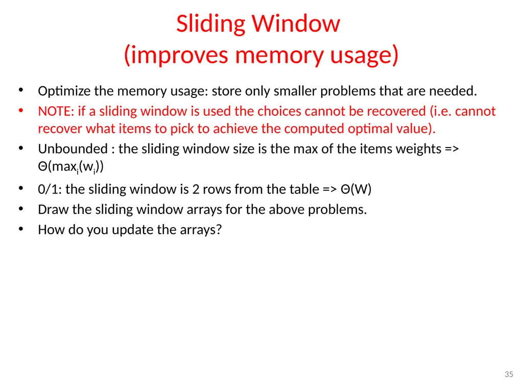
slide35. Sliding Window (improves memory usage) Optimize the memory usage: store only smaller problems that are needed.
NOTE: if a sliding window is used the choices cannot be recovered (i.e. cannot recover what items to pick to achieve the computed optimal value).
Unbounded : the sliding window size is the max of the items weights => Θ(maxi(wi))
0/1: the sliding window is 2 rows from the table => Θ(W)
Draw the sliding window arrays for the above problems.
How do you update the arrays? 35<br>
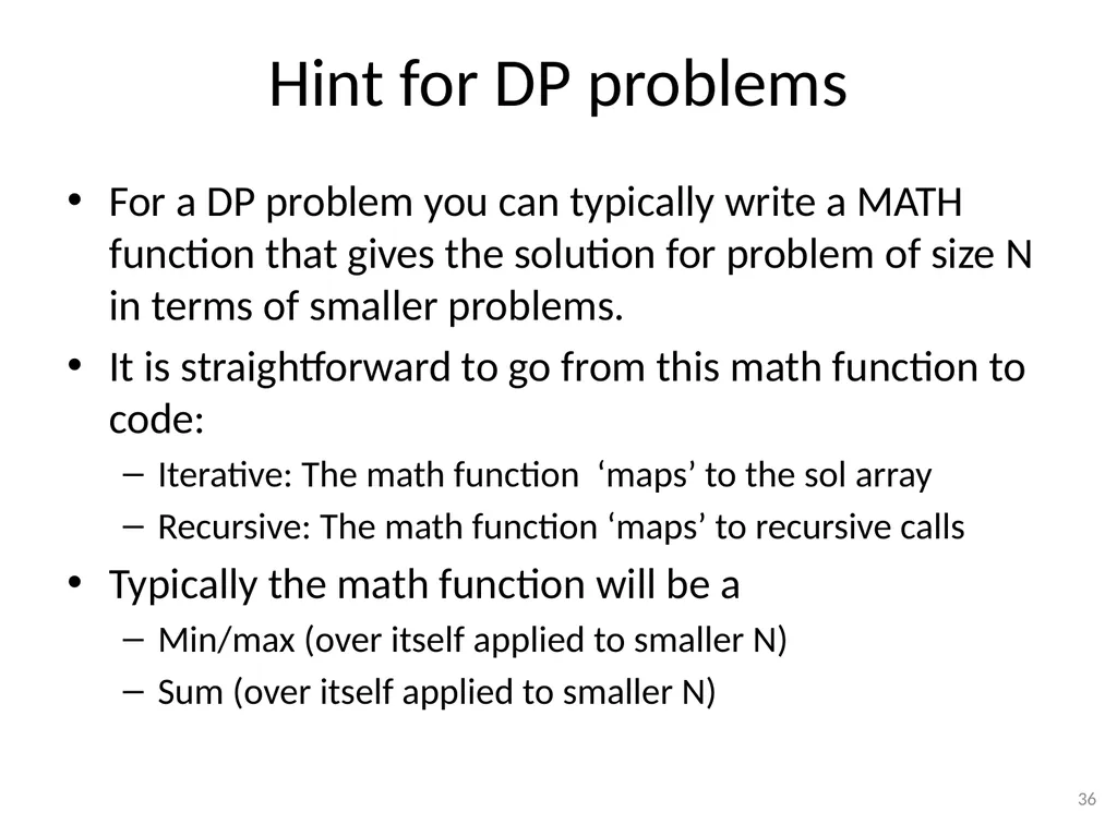
slide36. Hint for DP problems For a DP problem you can typically write a MATH function that gives the solution for problem of size N in terms of smaller problems.
It is straightforward to go from this math function to code:
Iterative: The math function ‘maps’ to the sol array
Recursive: The math function ‘maps’ to recursive calls
Typically the math function will be a
Min/max (over itself applied to smaller N)
Sum (over itself applied to smaller N) 36<br>
slide37. Weighted Interval Scheduling(Job Scheduling) 37<br>
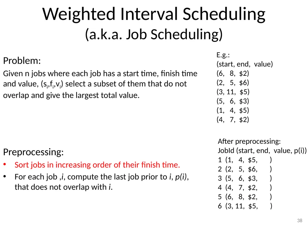
slide38. Weighted Interval Scheduling(a.k.a. Job Scheduling) Problem:
Given n jobs where each job has a start time, finish time and value, (si,fi,vi) select a subset of them that do not overlap and give the largest total value.

Preprocessing:
Sort jobs in increasing order of their finish time.
For each job ,i, compute the last job prior to i, p(i), that does not overlap with i. 38 E.g.:
(start, end, value)
(6, 8, $2)
(2, 5, $6)
(3, 11, $5)
(5, 6, $3)
(1, 4, $5)
(4, 7, $2) After preprocessing:
JobId (start, end, value, p(i))
1 (1, 4, $5, )
2 (2, 5, $6, )
3 (5, 6, $3, )
4 (4, 7, $2, )
5 (6, 8, $2, )
6 (3, 11, $5, )<br>
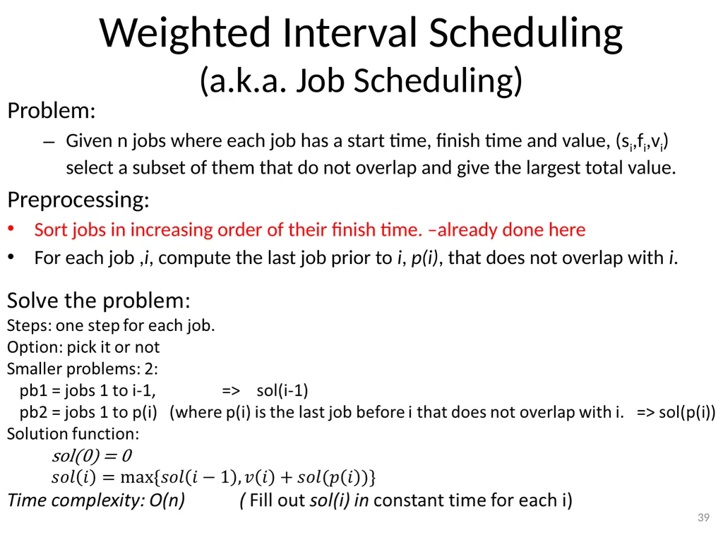
slide39. Weighted Interval Scheduling(a.k.a. Job Scheduling) Problem:
Given n jobs where each job has a start time, finish time and value, (si,fi,vi) select a subset of them that do not overlap and give the largest total value.
Preprocessing:
Sort jobs in increasing order of their finish time. –already done here
For each job ,i, compute the last job prior to i, p(i), that does not overlap with i. 39<br>
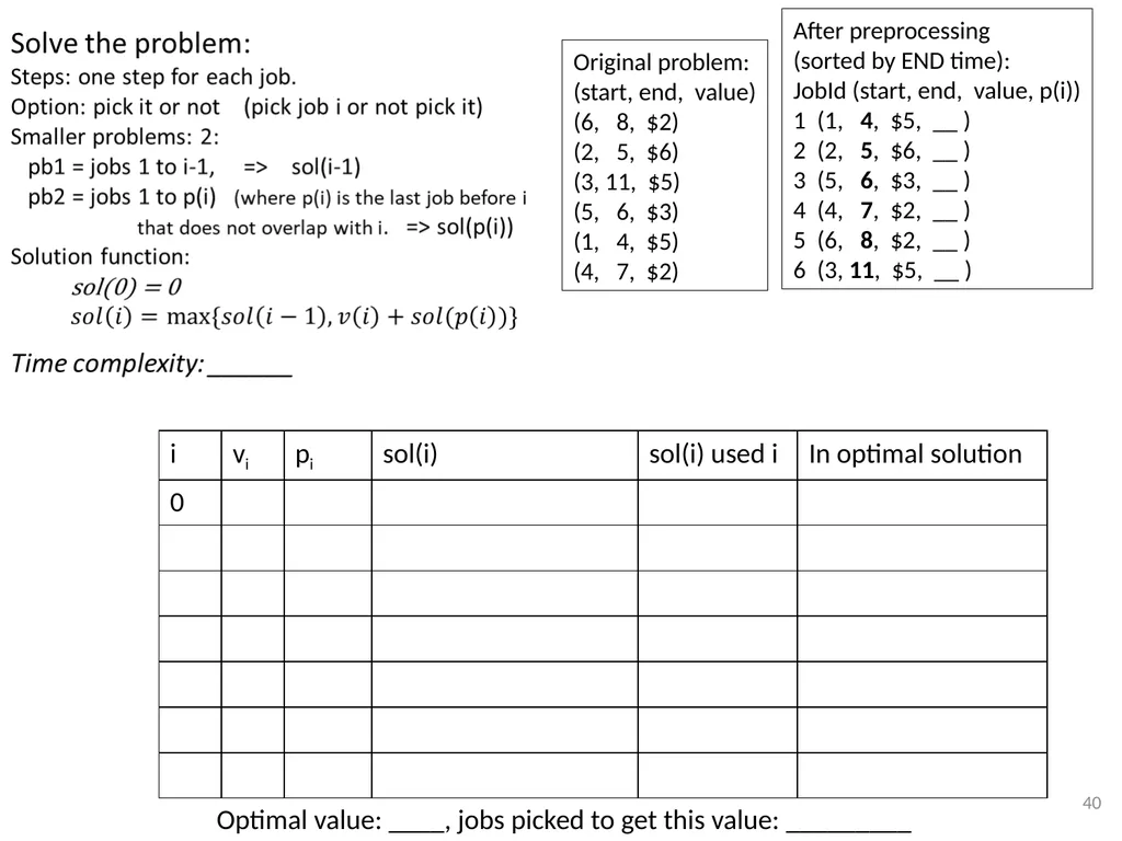
slide40. 40 Optimal value: ____, jobs picked to get this value: _________ Original problem:
(start, end, value)
(6, 8, $2)
(2, 5, $6)
(3, 11, $5)
(5, 6, $3)
(1, 4, $5)
(4, 7, $2) After preprocessing
(sorted by END time):
JobId (start, end, value, p(i))
1 (1, 4, $5, __ )
2 (2, 5, $6, __ )
3 (5, 6, $3, __ )
4 (4, 7, $2, __ )
5 (6, 8, $2, __ )
6 (3, 11, $5, __ )<br>
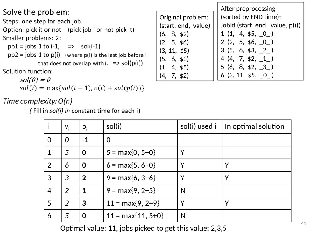
slide41. 41 Optimal value: 11, jobs picked to get this value: 2,3,5 Original problem:
(start, end, value)
(6, 8, $2)
(2, 5, $6)
(3, 11, $5)
(5, 6, $3)
(1, 4, $5)
(4, 7, $2) After preprocessing
(sorted by END time):
JobId (start, end, value, p(i))
1 (1, 4, $5, _0_ )
2 (2, 5, $6, _0_ )
3 (5, 6, $3, _2_ )
4 (4, 7, $2, _1_ )
5 (6, 8, $2, _3_ )
6 (3, 11, $5, _0_ )<br>
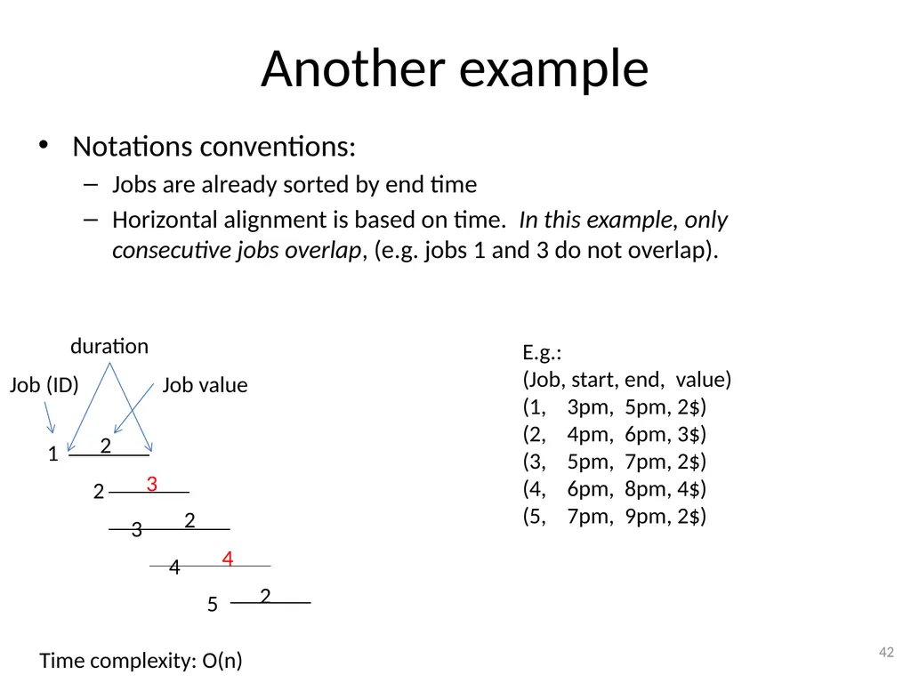
slide42. Another example Notations conventions:
Jobs are already sorted by end time
Horizontal alignment is based on time. In this example, only consecutive jobs overlap, (e.g. jobs 1 and 3 do not overlap). 42 2 3 2 4 2 1 2 3 4 5 Time complexity: O(n) Job value Job (ID) duration E.g.:
(Job, start, end, value)
(1, 3pm, 5pm, 2$)
(2, 4pm, 6pm, 3$)
(3, 5pm, 7pm, 2$)
(4, 6pm, 8pm, 4$)
(5, 7pm, 9pm, 2$)<br>
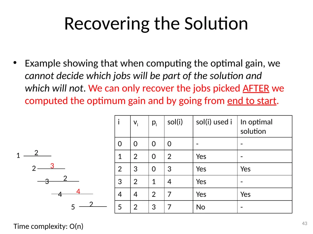
slide43. Recovering the Solution Example showing that when computing the optimal gain, we cannot decide which jobs will be part of the solution and which will not. We can only recover the jobs picked AFTER we computed the optimum gain and by going from end to start. 43 2 3 2 4 2 1 2 3 4 5 Time complexity: O(n)<br>
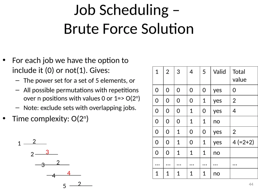
slide44. Job Scheduling – Brute Force Solution For each job we have the option to include it (0) or not(1). Gives:
The power set for a set of 5 elements, or
All possible permutations with repetitions over n positions with values 0 or 1=> O(2n)
Note: exclude sets with overlapping jobs.
Time complexity: O(2n) 44 2 3 2 4 2 1 2 3 4 5<br>
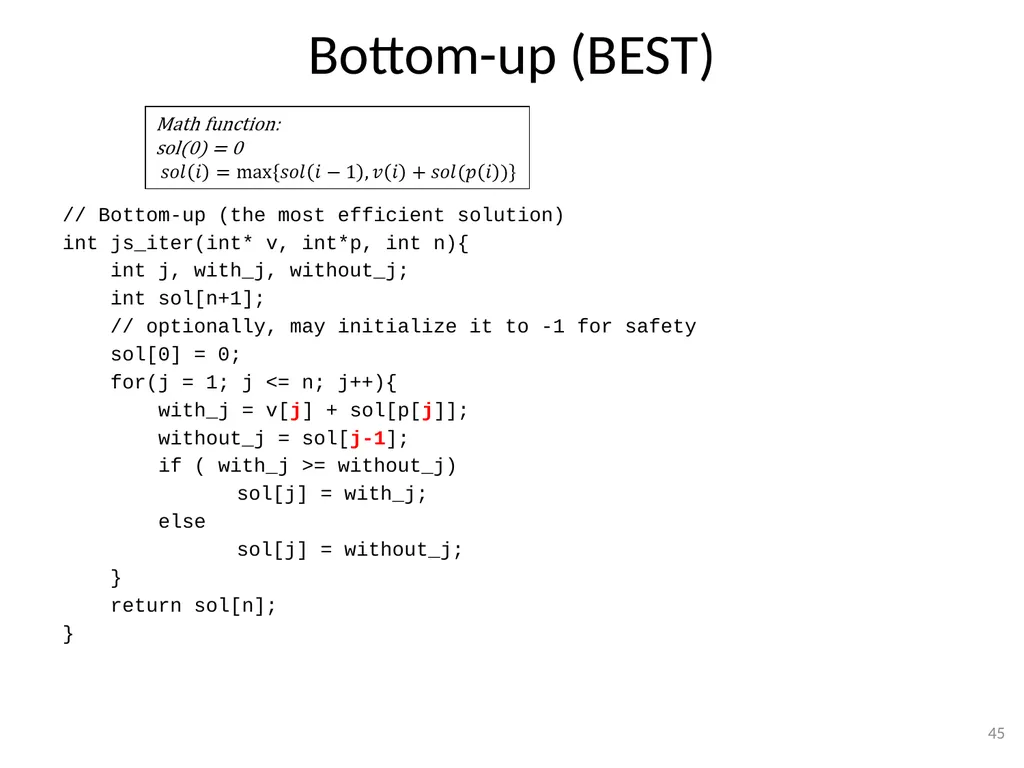
slide45. Bottom-up (BEST) // Bottom-up (the most efficient solution)
int js_iter(int* v, int*p, int n){
int j, with_j, without_j;
int sol[n+1];
// optionally, may initialize it to -1 for safety
sol[0] = 0;
for(j = 1; j <= n; j++){
with_j = v[j] + sol[p[j]];
without_j = sol[j-1];
if ( with_j >= without_j)
sol[j] = with_j;
else
sol[j] = without_j;
}
return sol[n];
} 45<br>
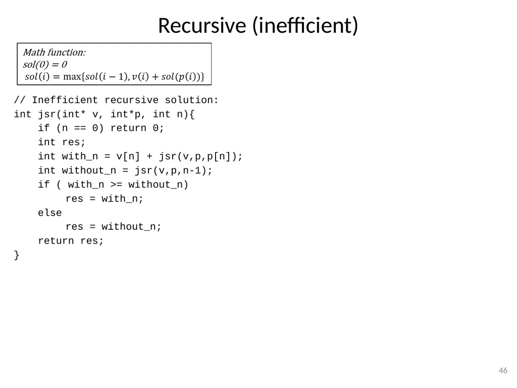
slide46. Recursive (inefficient) // Inefficient recursive solution:
int jsr(int* v, int*p, int n){
if (n == 0) return 0;
int res;
int with_n = v[n] + jsr(v,p,p[n]);
int without_n = jsr(v,p,n-1);
if ( with_n >= without_n)
res = with_n;
else
res = without_n;
return res;
} 46<br>
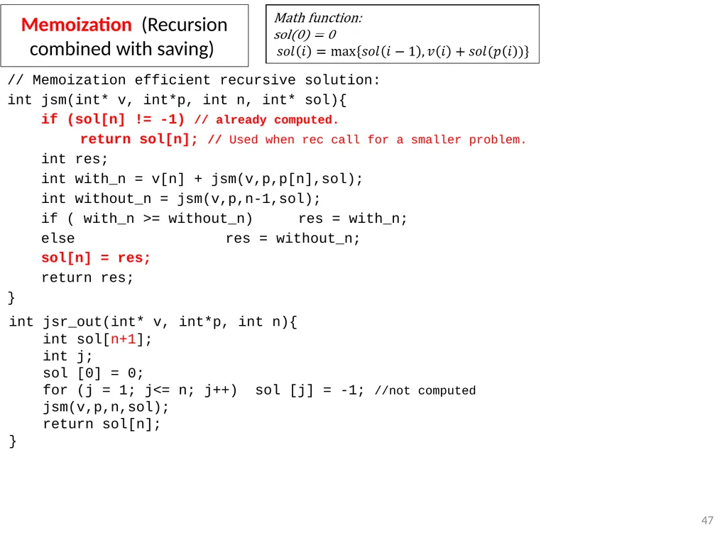
slide47. Memoization (Recursion combined with saving) // Memoization efficient recursive solution:
int jsm(int* v, int*p, int n, int* sol){
if (sol[n] != -1) // already computed.
return sol[n]; // Used when rec call for a smaller problem.
int res;
int with_n = v[n] + jsm(v,p,p[n],sol);
int without_n = jsm(v,p,n-1,sol);
if ( with_n >= without_n) res = with_n;
else res = without_n;
sol[n] = res;
return res;
} 47 int jsr_out(int* v, int*p, int n){
int sol[n+1];
int j;
sol [0] = 0;
for (j = 1; j<= n; j++) sol [j] = -1; //not computed
jsm(v,p,n,sol);
return sol[n];
}<br>
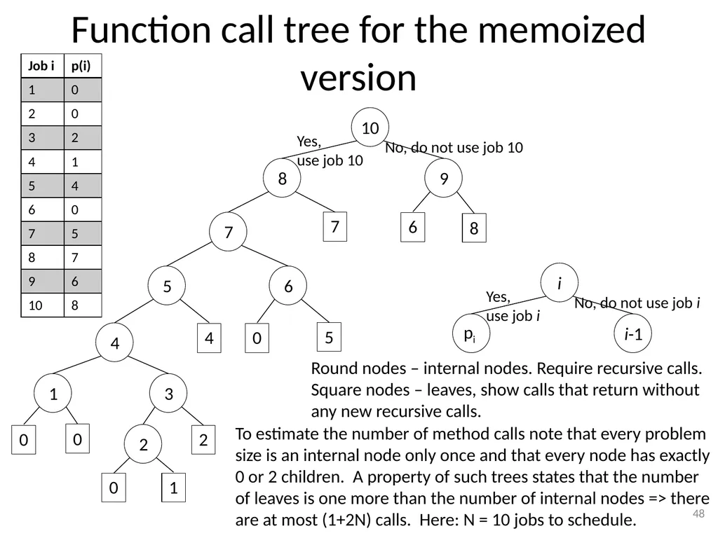
slide48. 48 10 9 8 6 8 7 7 6 5 5 0 4 4 1 3 0 0 2 0 1 2 Function call tree for the memoized version Round nodes – internal nodes. Require recursive calls.
Square nodes – leaves, show calls that return without any new recursive calls. Yes,
use job 10 No, do not use job 10 i i-1 pi Yes,
use job i No, do not use job i To estimate the number of method calls note that every problem size is an internal node only once and that every node has exactly 0 or 2 children. A property of such trees states that the number of leaves is one more than the number of internal nodes => there are at most (1+2N) calls. Here: N = 10 jobs to schedule.<br>
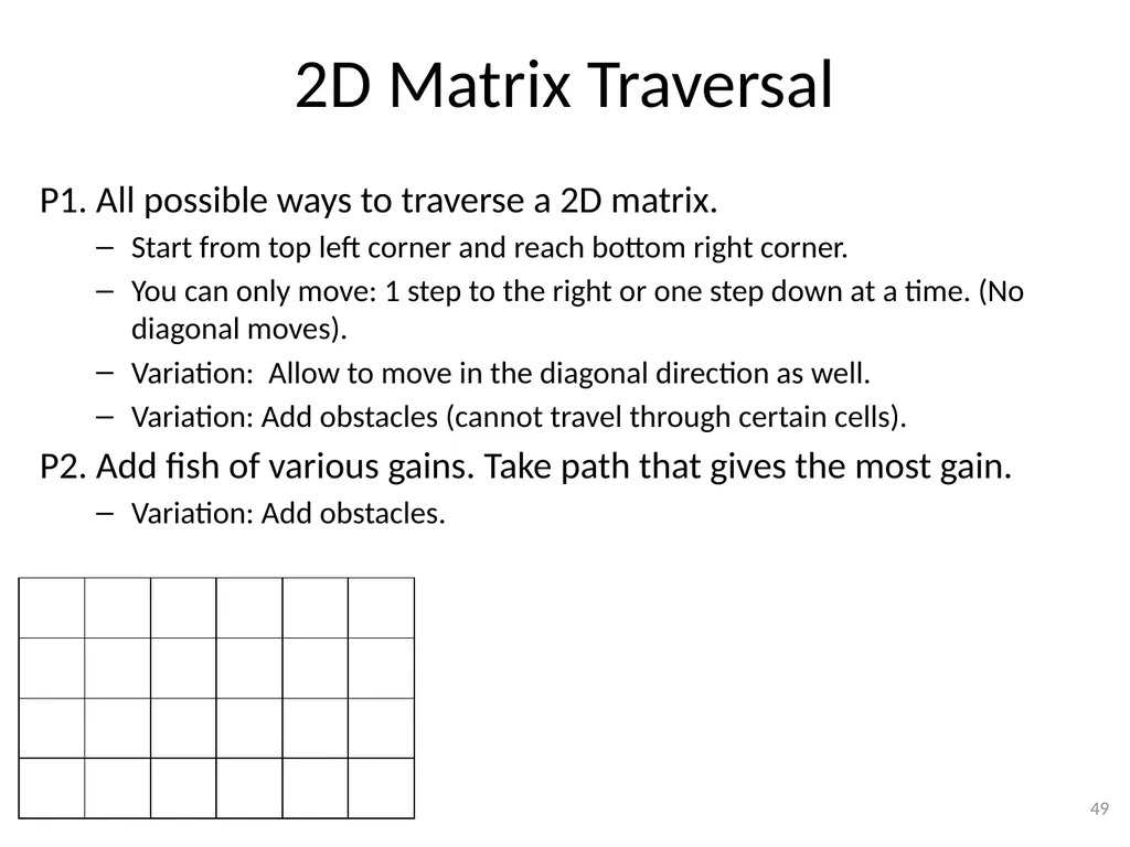
slide49. 2D Matrix Traversal P1. All possible ways to traverse a 2D matrix.
Start from top left corner and reach bottom right corner.
You can only move: 1 step to the right or one step down at a time. (No diagonal moves).
Variation: Allow to move in the diagonal direction as well.
Variation: Add obstacles (cannot travel through certain cells).
P2. Add fish of various gains. Take path that gives the most gain.
Variation: Add obstacles. 49<br>
slide50. Longest Common Subsequence(LCS) 50<br>
slide51. Longest Common Subsequence (LCS) Given 2 sequences, find the longest common subsequence (LCS)
Example:
A B C B D A B
B D C A B A
Examples of subsequences of the above sequences:
BCBA (length 4)
BDAB
CBA (length 3)
CAB
BB (length 2) 51 Show the components of the solution.
Can you show a solution similar that of an Edit distance problem?<br>
slide52. LCSSmaller Problems Original problem:
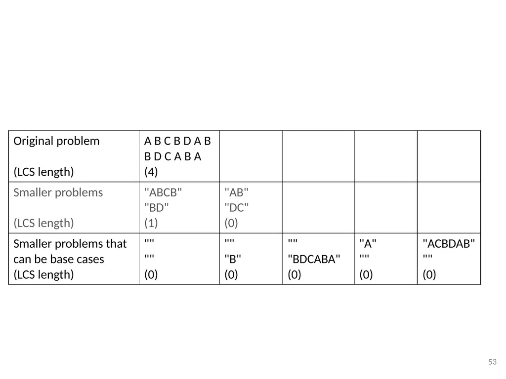
A B C B D A B
B D C A B A
Smaller problems:

Smaller problems that can be base cases: 52<br>
slide53. 53<br>
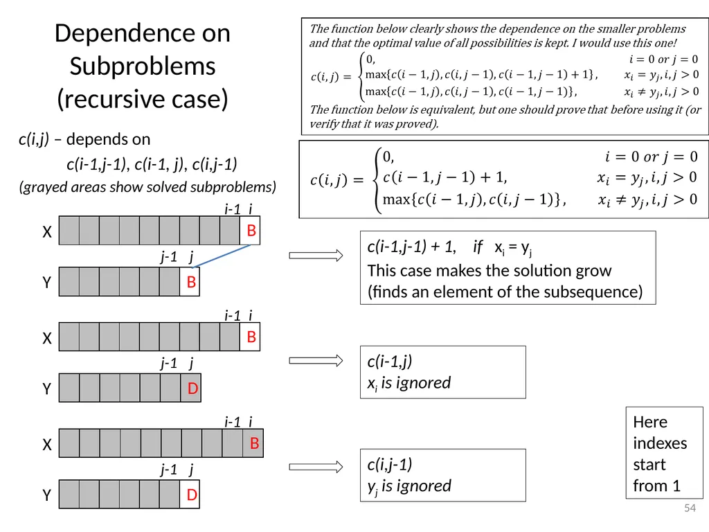
slide54. Dependence on Subproblems(recursive case) c(i,j) – depends on
c(i-1,j-1), c(i-1, j), c(i,j-1)
(grayed areas show solved subproblems) 54 X Y i j j-1 i-1 X Y i j j-1 i-1 X Y i j j-1 i-1 c(i-1,j-1) + 1, if xi = yj
This case makes the solution grow
(finds an element of the subsequence) c(i-1,j)
xi is ignored c(i,j-1)
yj is ignored Here indexes start from 1<br>
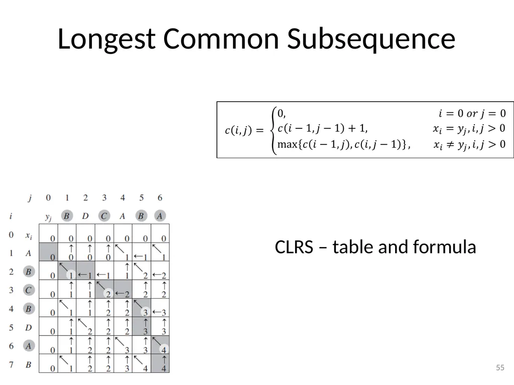
slide55. Longest Common Subsequence CLRS – table and formula 55<br>
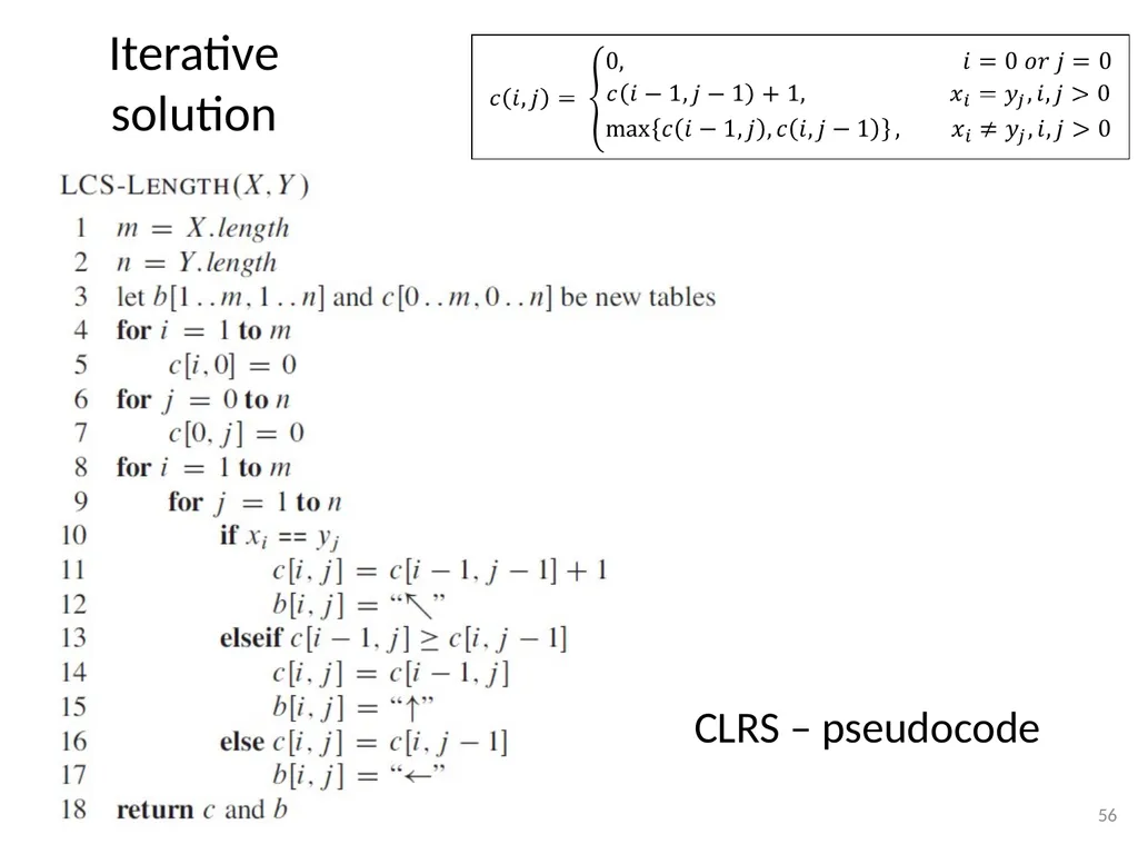
slide56. Iterative solution 56 CLRS – pseudocode<br>
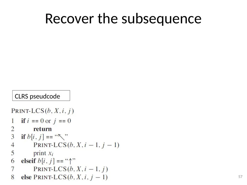
slide57. Recover the subsequence CLRS pseudcode 57<br>
slide58. Longest Increasing Subsequence(LIS) 58<br>
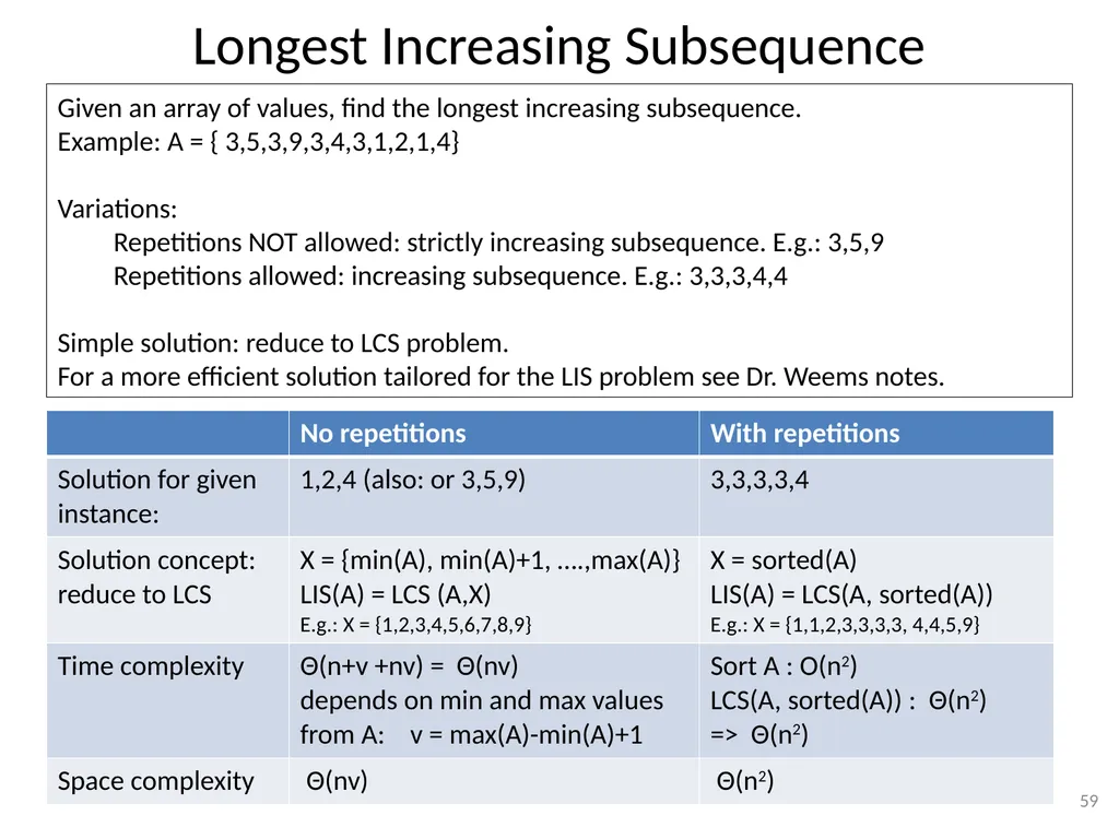
slide59. 59 Given an array of values, find the longest increasing subsequence.
Example: A = { 3,5,3,9,3,4,3,1,2,1,4}

Variations:
Repetitions NOT allowed: strictly increasing subsequence. E.g.: 3,5,9
Repetitions allowed: increasing subsequence. E.g.: 3,3,3,4,4

Simple solution: reduce to LCS problem.
For a more efficient solution tailored for the LIS problem see Dr. Weems notes. Longest Increasing Subsequence<br>
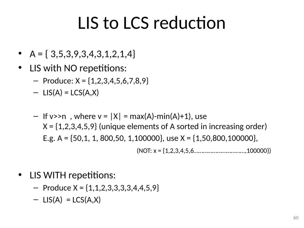
slide60. LIS to LCS reduction A = { 3,5,3,9,3,4,3,1,2,1,4}
LIS with NO repetitions:
Produce: X = {1,2,3,4,5,6,7,8,9}
LIS(A) = LCS(A,X)

If v>>n , where v = |X| = max(A)-min(A)+1), use X = {1,2,3,4,5,9} (unique elements of A sorted in increasing order)
E.g. A = {50,1, 1, 800,50, 1,100000}, use X = {1,50,800,100000},
(NOT: x = {1,2,3,4,5,6……………………………,100000})

LIS WITH repetitions:
Produce X = {1,1,2,3,3,3,3,4,4,5,9}
LIS(A) = LCS(A,X) 60<br>
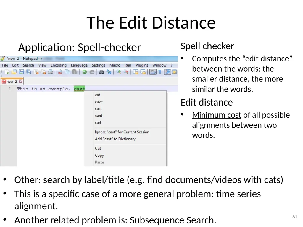
slide61. The Edit Distance Application: Spell-checker 61 Other: search by label/title (e.g. find documents/videos with cats)
This is a specific case of a more general problem: time series alignment.
Another related problem is: Subsequence Search. Spell checker
Computes the “edit distance” between the words: the smaller distance, the more similar the words.
Edit distance
Minimum cost of all possible alignments between two words.<br>
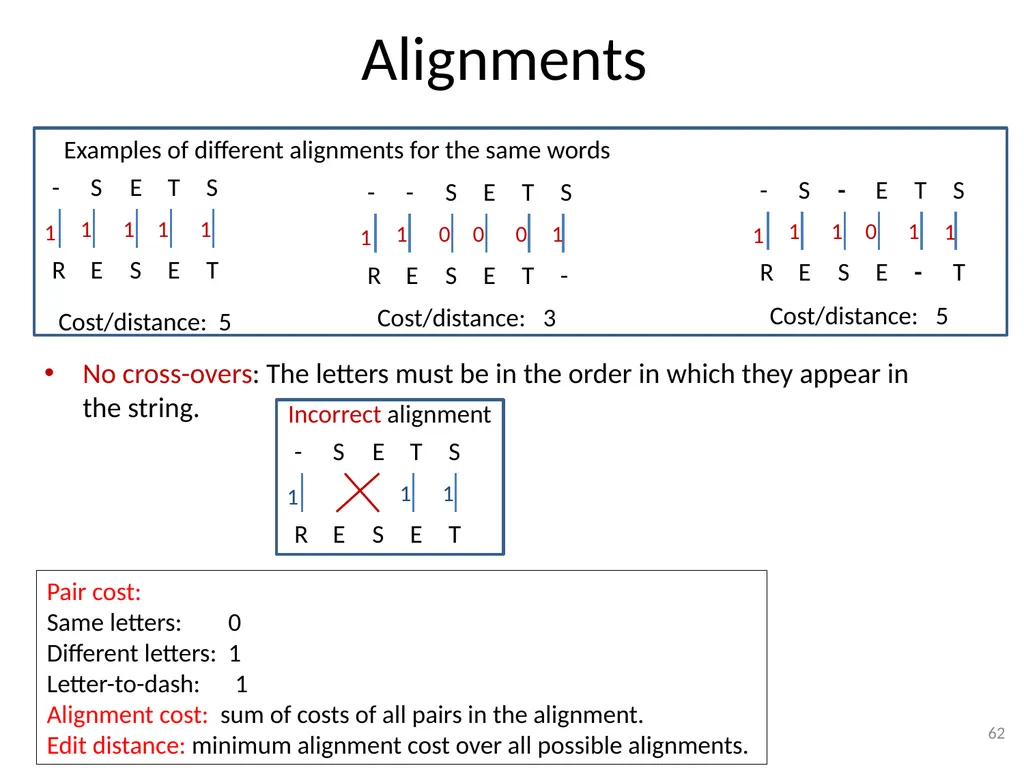
slide62. Alignments 62 1 1 1 0 0 0 1 1 1 1 1 Cost/distance: 5 Cost/distance: 3 No cross-overs: The letters must be in the order in which they appear in the string. Examples of different alignments for the same words 1 1 1 Incorrect alignment 1 1 1 1 0 1 Cost/distance: 5 Pair cost:
Same letters: 0
Different letters: 1
Letter-to-dash: 1
Alignment cost: sum of costs of all pairs in the alignment.
Edit distance: minimum alignment cost over all possible alignments.<br>
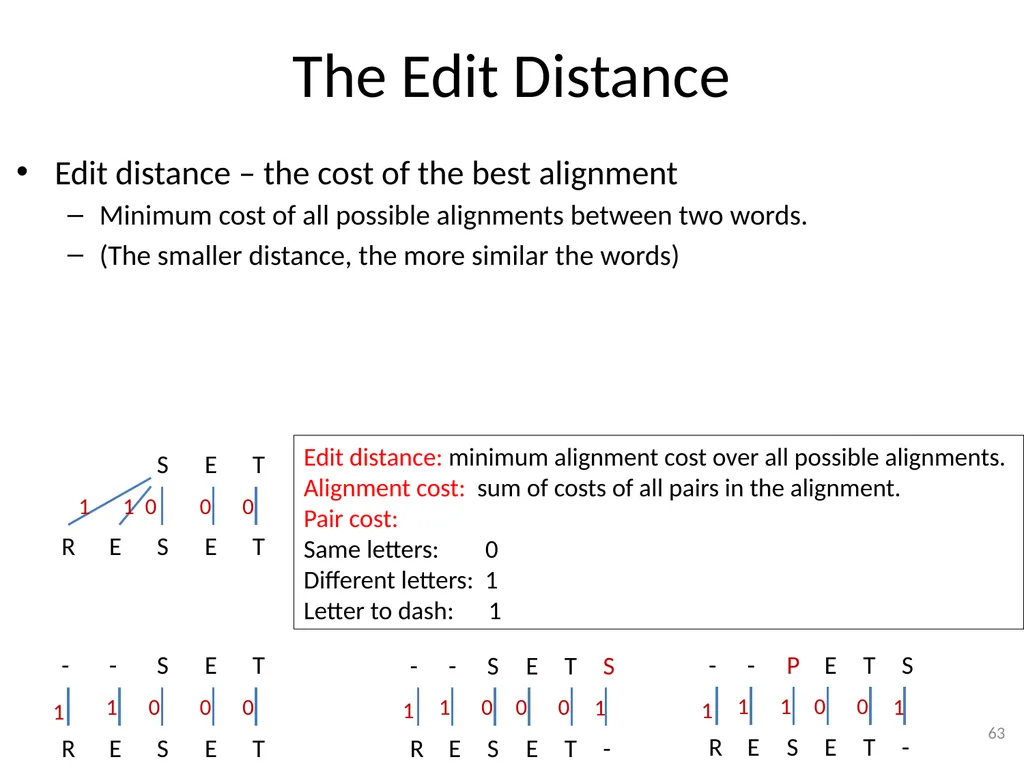
slide63. The Edit Distance Edit distance – the cost of the best alignment
Minimum cost of all possible alignments between two words.
(The smaller distance, the more similar the words) 63 1 1 1 0 0 0 1 1 0 0 0 1 1 1 1 0 0 1 1 0 0 0 Edit distance: minimum alignment cost over all possible alignments.
Alignment cost: sum of costs of all pairs in the alignment.
Pair cost:
Same letters: 0
Different letters: 1
Letter to dash: 1<br>
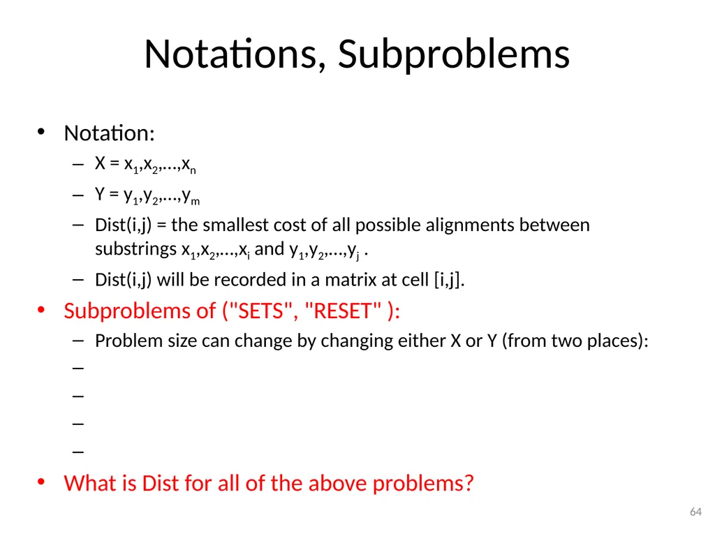
slide64. Notations, Subproblems Notation:
X = x1,x2,…,xn
Y = y1,y2,…,ym
Dist(i,j) = the smallest cost of all possible alignments between substrings x1,x2,…,xi and y1,y2,…,yj .
Dist(i,j) will be recorded in a matrix at cell [i,j].
Subproblems of ("SETS", "RESET" ):
Problem size can change by changing either X or Y (from two places):




What is Dist for all of the above problems? 64<br>
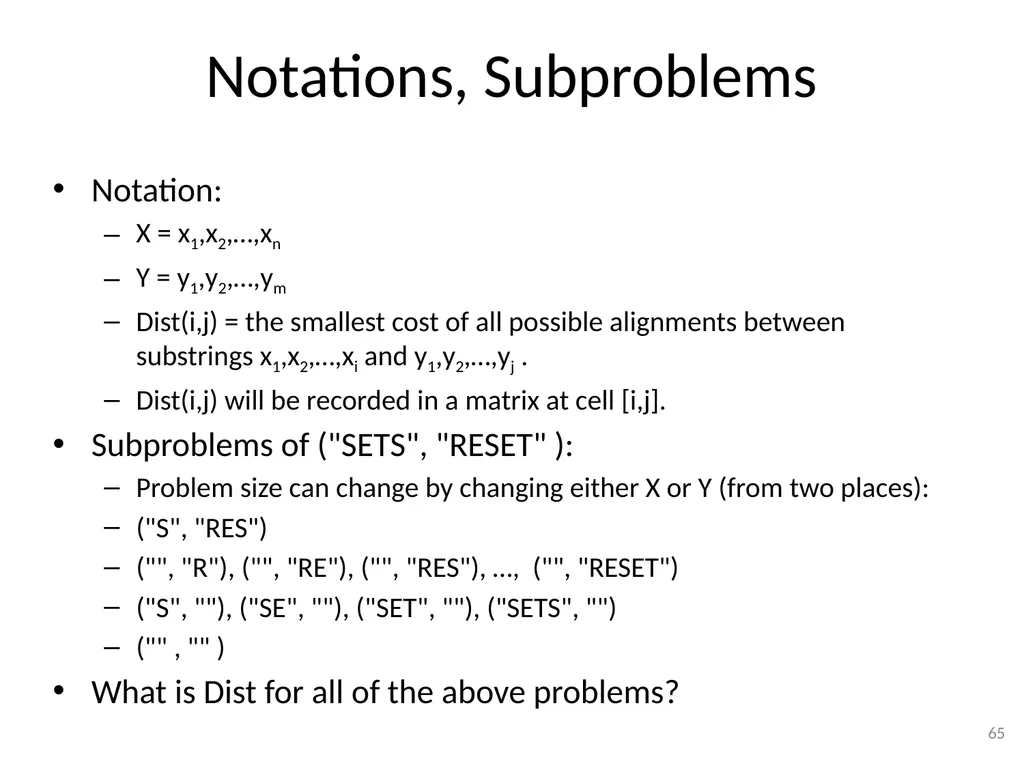
slide65. Notations, Subproblems Notation:
X = x1,x2,…,xn
Y = y1,y2,…,ym
Dist(i,j) = the smallest cost of all possible alignments between substrings x1,x2,…,xi and y1,y2,…,yj .
Dist(i,j) will be recorded in a matrix at cell [i,j].
Subproblems of ("SETS", "RESET" ):
Problem size can change by changing either X or Y (from two places):
("S", "RES")
("", "R"), ("", "RE"), ("", "RES"), …, ("", "RESET")
("S", ""), ("SE", ""), ("SET", ""), ("SETS", "")
("" , "" )
What is Dist for all of the above problems? 65<br>
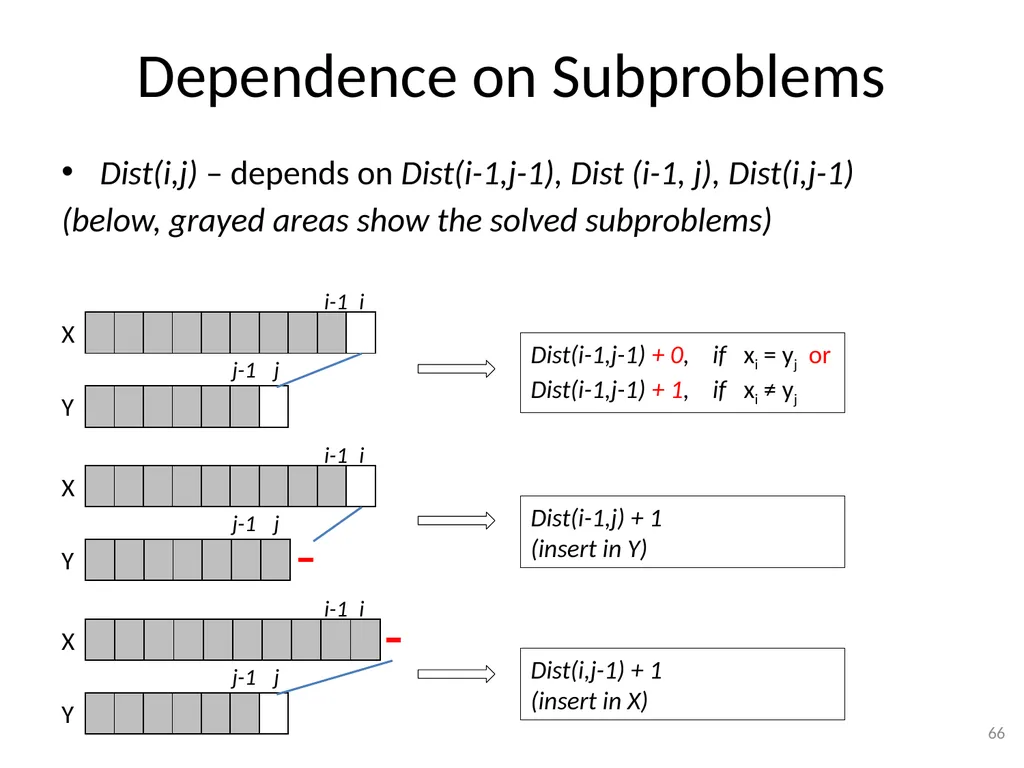
slide66. Dependence on Subproblems Dist(i,j) – depends on Dist(i-1,j-1), Dist (i-1, j), Dist(i,j-1)
(below, grayed areas show the solved subproblems) 66 X Y i j j-1 i-1 X Y i j j-1 i-1 X Y i j j-1 i-1 Dist(i-1,j-1) + 0, if xi = yj or
Dist(i-1,j-1) + 1, if xi ≠ yj Dist(i-1,j) + 1
(insert in Y) Dist(i,j-1) + 1
(insert in X)<br>
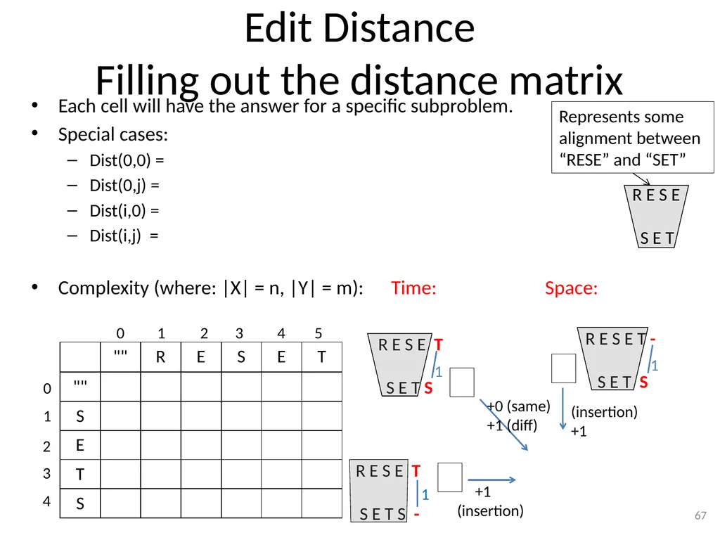
slide67. Edit DistanceFilling out the distance matrix Each cell will have the answer for a specific subproblem.
Special cases:
Dist(0,0) =
Dist(0,j) =
Dist(i,0) =
Dist(i,j) =

Complexity (where: |X| = n, |Y| = m): Time: Space: 67 (insertion)
+1 +1
(insertion) +0 (same)
+1 (diff) 0 1 2 3 4 0 1 2 3 4 5 R E S E T -

S E T S 1 R E S E T

S E T S - 1 R E S E T

S E T S 1 R E S E

S E T Represents some alignment between “RESE” and “SET”<br>
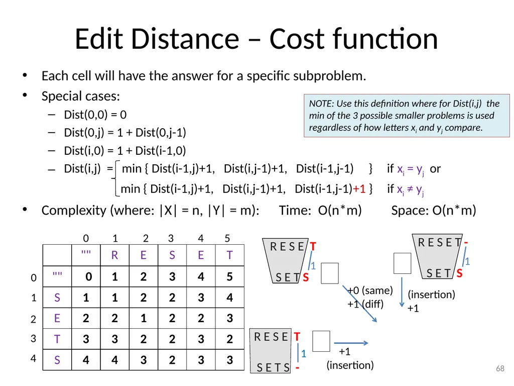
slide68. Edit Distance – Cost function Each cell will have the answer for a specific subproblem.
Special cases:
Dist(0,0) = 0
Dist(0,j) = 1 + Dist(0,j-1)
Dist(i,0) = 1 + Dist(i-1,0)
Dist(i,j) = min { Dist(i-1,j)+1, Dist(i,j-1)+1, Dist(i-1,j-1) } if xi = yj or
min { Dist(i-1,j)+1, Dist(i,j-1)+1, Dist(i-1,j-1)+1 } if xi ≠ yj
Complexity (where: |X| = n, |Y| = m): Time: O(n*m) Space: O(n*m) 68 0 1 2 3 4 0 1 2 3 4 5 (insertion)
+1 +1
(insertion) +0 (same)
+1 (diff) R E S E T -

S E T S 1 R E S E T

S E T S - 1 R E S E T

S E T S 1 NOTE: Use this definition where for Dist(i,j) the min of the 3 possible smaller problems is used regardless of how letters xi and yj compare.<br>
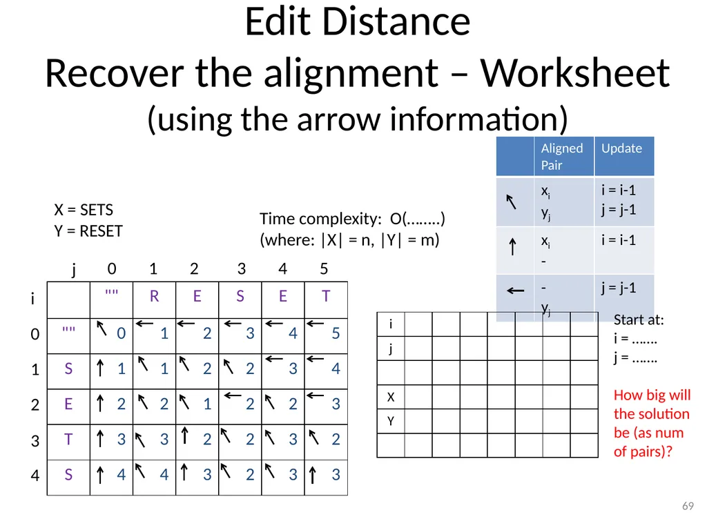
slide69. Edit DistanceRecover the alignment – Worksheet(using the arrow information) 69 0 1 2 3 0 1 2 3 4 5 Start at:
i = …….
j = …….

How big will the solution be (as num of pairs)? X = SETS
Y = RESET 4 Time complexity: O(……..)
(where: |X| = n, |Y| = m) i j<br>
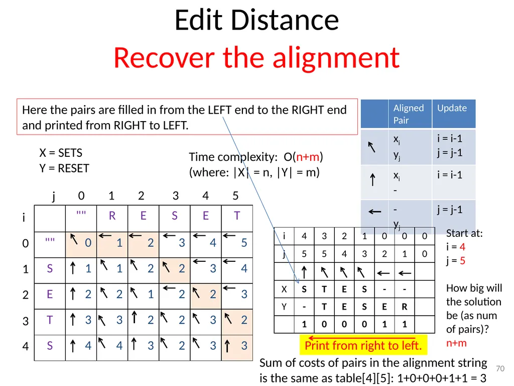
slide70. Edit DistanceRecover the alignment 70 0 1 2 3 0 1 2 3 4 5 Start at:
i = 4
j = 5

How big will the solution be (as num of pairs)?
n+m X = SETS
Y = RESET 4 Time complexity: O(n+m)
(where: |X| = n, |Y| = m) i j Print from right to left. Here the pairs are filled in from the LEFT end to the RIGHT end and printed from RIGHT to LEFT. Sum of costs of pairs in the alignment string
is the same as table[4][5]: 1+0+0+0+1+1 = 3<br>
slide71. What is the best alignment between
abcdefghijk
cdXYZefgh 71<br>
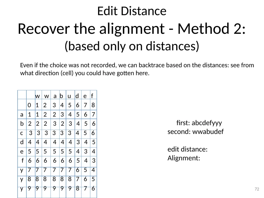
slide72. w w a b u d e f
0 1 2 3 4 5 6 7 8
a 1 1 2 2 3 4 5 6 7
b 2 2 2 3 2 3 4 5 6
c 3 3 3 3 3 3 4 5 6
d 4 4 4 4 4 4 3 4 5
e 5 5 5 5 5 5 4 3 4
f 6 6 6 6 6 6 5 4 3
y 7 7 7 7 7 7 6 5 4
y 8 8 8 8 8 8 7 6 5
y 9 9 9 9 9 9 8 7 6 72 first: abcdefyyy
second: wwabudef

edit distance:
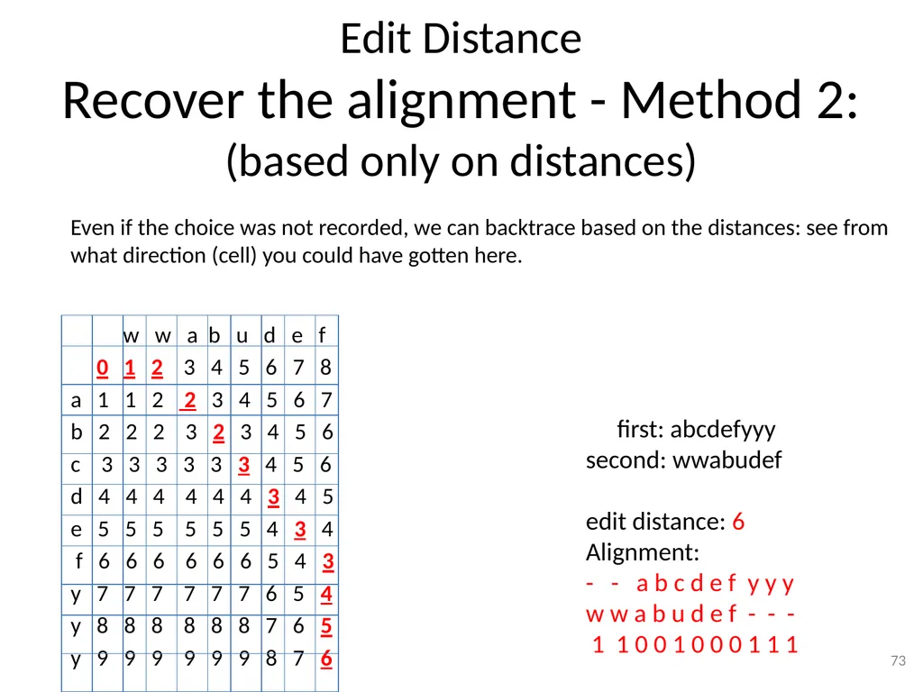
Alignment: Even if the choice was not recorded, we can backtrace based on the distances: see from what direction (cell) you could have gotten here. Edit DistanceRecover the alignment - Method 2:(based only on distances)<br>
slide73. Edit DistanceRecover the alignment - Method 2:(based only on distances) w w a b u d e f
0 1 2 3 4 5 6 7 8
a 1 1 2 2 3 4 5 6 7
b 2 2 2 3 2 3 4 5 6
c 3 3 3 3 3 3 4 5 6
d 4 4 4 4 4 4 3 4 5
e 5 5 5 5 5 5 4 3 4
f 6 6 6 6 6 6 5 4 3
y 7 7 7 7 7 7 6 5 4
y 8 8 8 8 8 8 7 6 5
y 9 9 9 9 9 9 8 7 6 73 first: abcdefyyy
second: wwabudef

edit distance: 6
Alignment:
- - a b c d e f y y y
w w a b u d e f - - -
1 1 0 0 1 0 0 0 1 1 1 Even if the choice was not recorded, we can backtrace based on the distances: see from what direction (cell) you could have gotten here.<br>
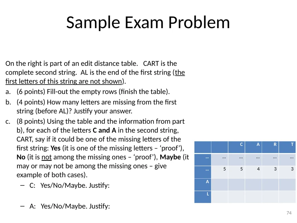
slide74. Sample Exam Problem On the right is part of an edit distance table. CART is the complete second string. AL is the end of the first string (the first letters of this string are not shown).
(6 points) Fill-out the empty rows (finish the table).
(4 points) How many letters are missing from the first string (before AL)? Justify your answer. 
(8 points) Using the table and the information from part b), for each of the letters C and A in the second string, CART, say if it could be one of the missing letters of the first string: Yes (it is one of the missing letters – ‘proof’), No (it is not among the missing ones – ‘proof’), Maybe (it may or may not be among the missing ones – give example of both cases).
C: Yes/No/Maybe. Justify:

A: Yes/No/Maybe. Justify: 74<br>
slide75. Edit Distance Sliding Window Space complexity improvement:
Keep only two rows

Keep only one row 75<br>
slide76. Motivation for Edit Distance The Edit Distance essentially does Time Series Alignment
Other examples of problems solved with Time Series Alignment:
Given observed temperatures, find location:
Collected in a database temperatures at different hours over one day in various places (labelled with the name). Given a query consisting of temperatures collected in an unknown place, find the place with the most similar temperatures. Issues:
Not same number of measurements for every place and query.
Not at the exact same time. (E.g. maybe Mary recorded more temperatures throughout the day and none in the night, and John collected uniformly throughout the day and night.)
Find videos showing a similar sign
Find shapes in images (after image processing extracted relevant features)
Find a substring in a string
E.g. swear words in Pokemon Names
Uses two additional sink states (at the beginning and end of the small query) 76<br>
slide77. DP in an exam Must be able to solve these problems in the shown format and with the methods covered in class.
Components of every DP problem:
Problem description and representation,
Cost function (math formulation and/or implementation), recover the solution, brute force method
time complexity for all three items above
Solve on paper:
Find optimum.
Recover choices that give optimum solution. 77<br>
slide78. DP or not DP? I consider DP problems to be optimization problems.
CLRS gives only optimization problems as DP
Other sources list non-optimization problems as DP as well.
Main point: optimization problems are hard. Consider DP for them.

DP requires two properties:
Optimal substructure – applicable to optimization problems
An optimal solution to the big problem can be constructed from optimal solutions to smaller problems.
Overlapping subproblems – applicable to all problems (including Fibonacci, stair climbing, matrix traversal)
The pattern of the solution in both cases (e.g. matrix traversal with and without optimization) is the same except that in one case you add the answer from the subproblems and in the other you pick the max.
Results in an ordering of the subproblems, where each next depends on the previous ones. 78<br>
slide79. Divide and Conquer vs DP vs Recursion Both DP and Divide and Conquer can be easily solved using recursion
For Divide and conquer you typically want to use recursion (ok if you do)
For DP you want to use memoization or the iterative solution (recursion is exponential)
Recursive problem that does not allow neither DP nor Div & Conq:
Place N queens on an NxN check board (s.t. they do not attack each other)
Divide and conquer problems:
Sum of elements in an array
Give the solution here
Factorial with splitting in half (or Sorting elements in an array (Mergesort))
Notes:
Problems of same size (e.g. 3 elements) are different (depending on the actual values and order of the elements). => cannot ‘reuse’ solutions to smaller problems.
Unlike DP, the solution does not depend on where we cut (ok to cut into subproblems at any place)
Why Dynamic Programming (DP) and not Divide and Conquer
We cannot apply Div&Conq because we cannot commit to a ‘point’ in the solution (e.g. , for Job Scheduling, choose if a certain job will be selected or not). 79<br>
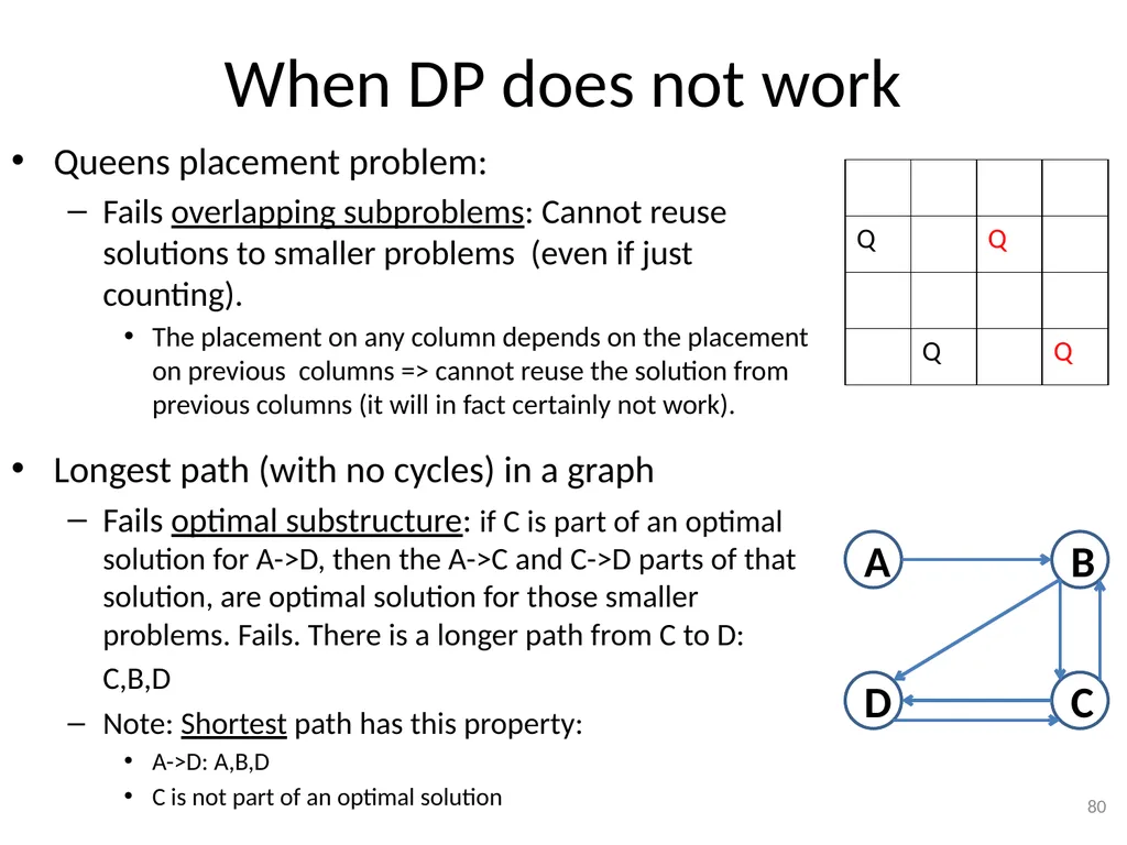
slide80. When DP does not work Queens placement problem:
Fails overlapping subproblems: Cannot reuse solutions to smaller problems (even if just counting).
The placement on any column depends on the placement on previous columns => cannot reuse the solution from previous columns (it will in fact certainly not work).

Longest path (with no cycles) in a graph
Fails optimal substructure: if C is part of an optimal solution for A->D, then the A->C and C->D parts of that solution, are optimal solution for those smaller problems. Fails. There is a longer path from C to D: C,B,D
Note: Shortest path has this property:
A->D: A,B,D
C is not part of an optimal solution 80<br>
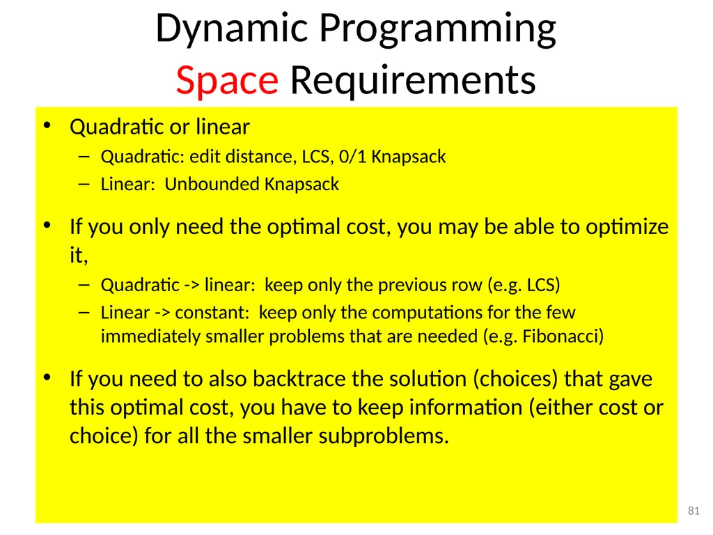
slide81. Dynamic ProgrammingSpace Requirements Quadratic or linear
Quadratic: edit distance, LCS, 0/1 Knapsack
Linear: Unbounded Knapsack

If you only need the optimal cost, you may be able to optimize it,
Quadratic -> linear: keep only the previous row (e.g. LCS)
Linear -> constant: keep only the computations for the few immediately smaller problems that are needed (e.g. Fibonacci)

If you need to also backtrace the solution (choices) that gave this optimal cost, you have to keep information (either cost or choice) for all the smaller subproblems. 81<br>
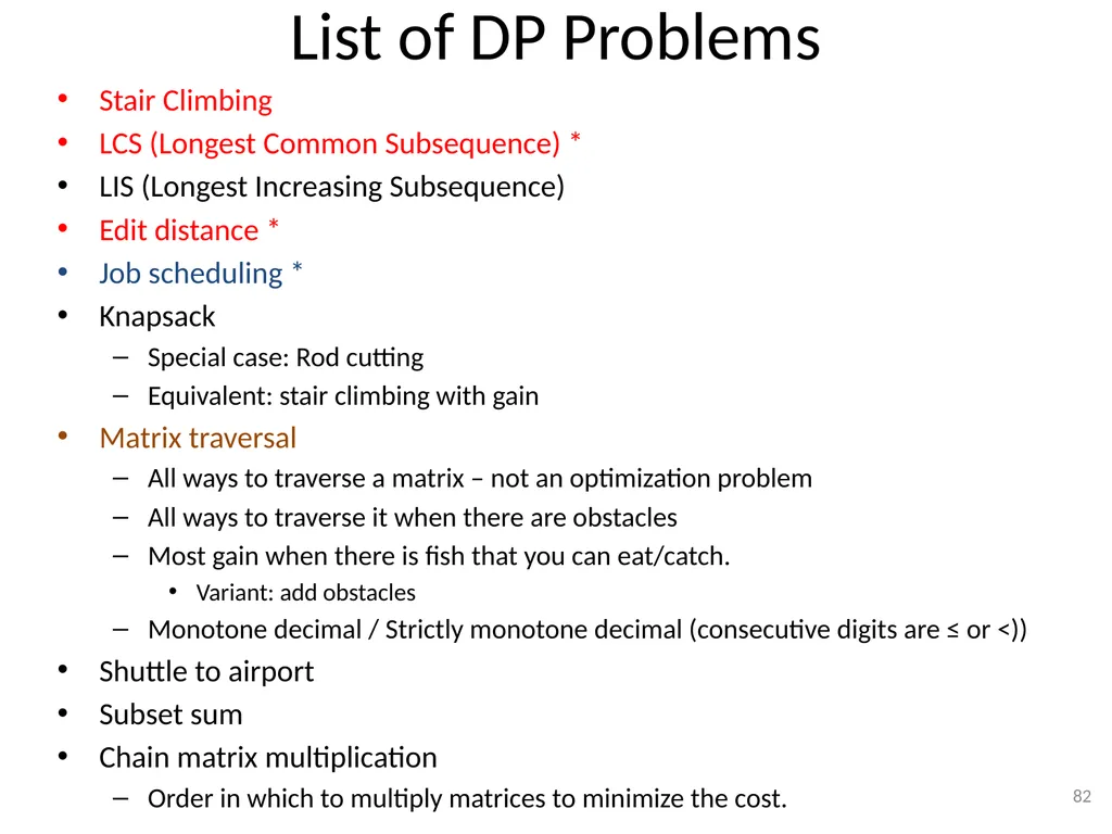
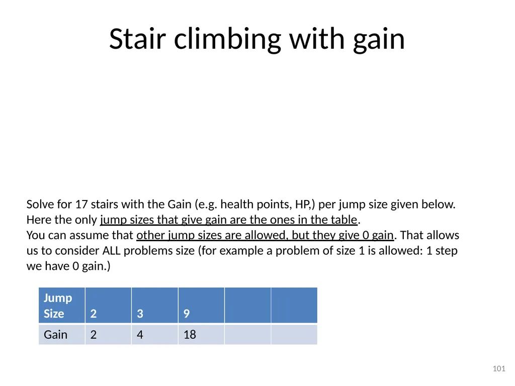
slide82. List of DP Problems Stair Climbing
LCS (Longest Common Subsequence) *
LIS (Longest Increasing Subsequence)
Edit distance *
Job scheduling *
Knapsack
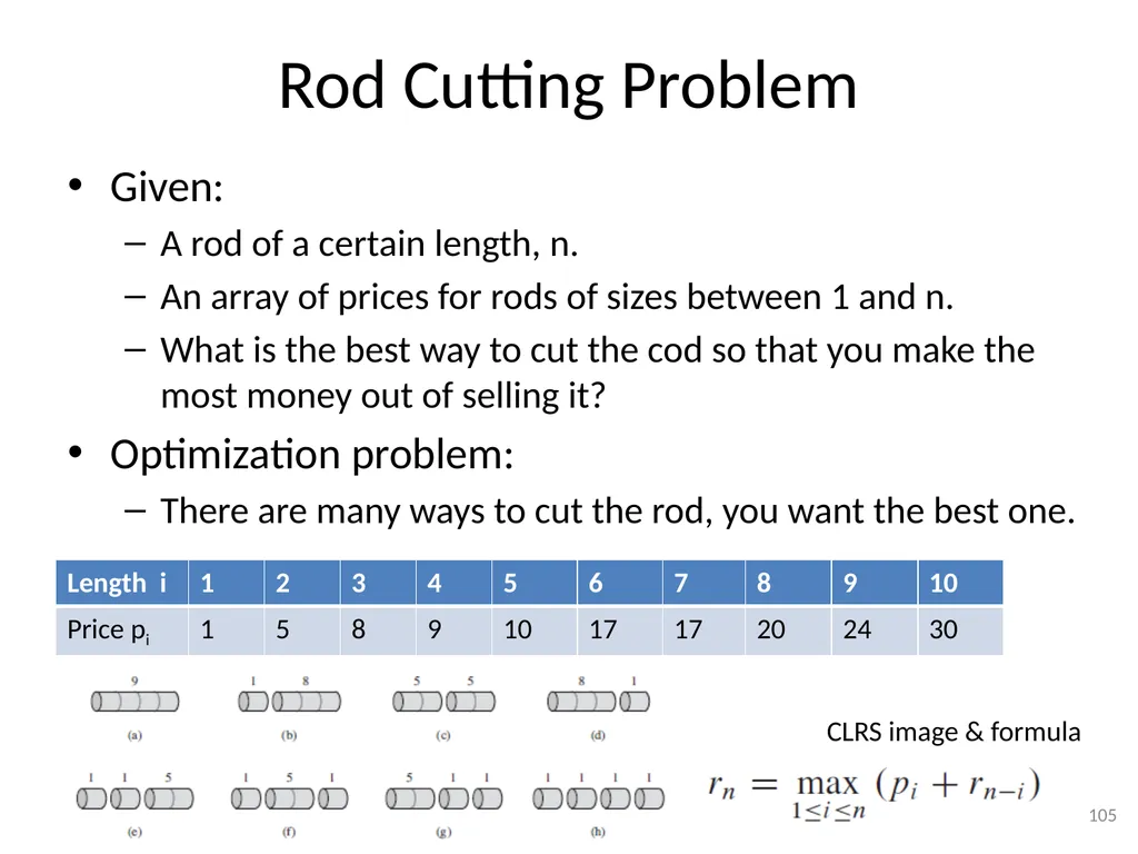
Special case: Rod cutting
Equivalent: stair climbing with gain
Matrix traversal
All ways to traverse a matrix – not an optimization problem
All ways to traverse it when there are obstacles
Most gain when there is fish that you can eat/catch.
Variant: add obstacles
Monotone decimal / Strictly monotone decimal (consecutive digits are ≤ or <))
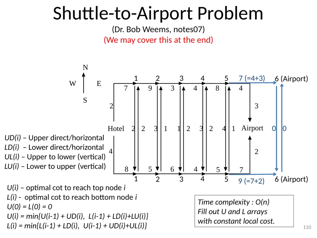
Shuttle to airport
Subset sum
Chain matrix multiplication
Order in which to multiply matrices to minimize the cost. 82<br>
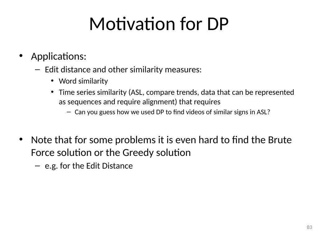
slide83. Motivation for DP Applications:
Edit distance and other similarity measures:
Word similarity
Time series similarity (ASL, compare trends, data that can be represented as sequences and require alignment) that requires
Can you guess how we used DP to find videos of similar signs in ASL?

Note that for some problems it is even hard to find the Brute Force solution or the Greedy solution
e.g. for the Edit Distance 83<br>
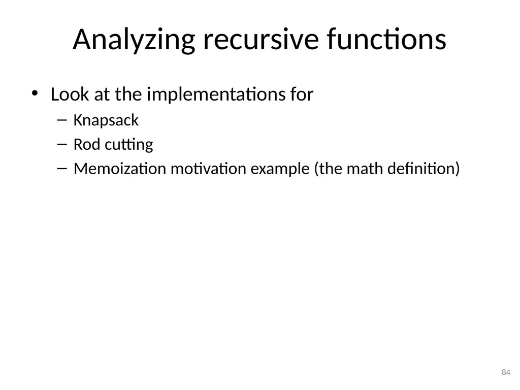
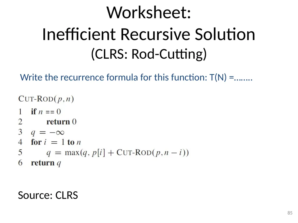
slide84. Analyzing recursive functions Look at the implementations for
Knapsack
Rod cutting
Memoization motivation example (the math definition) 84<br>
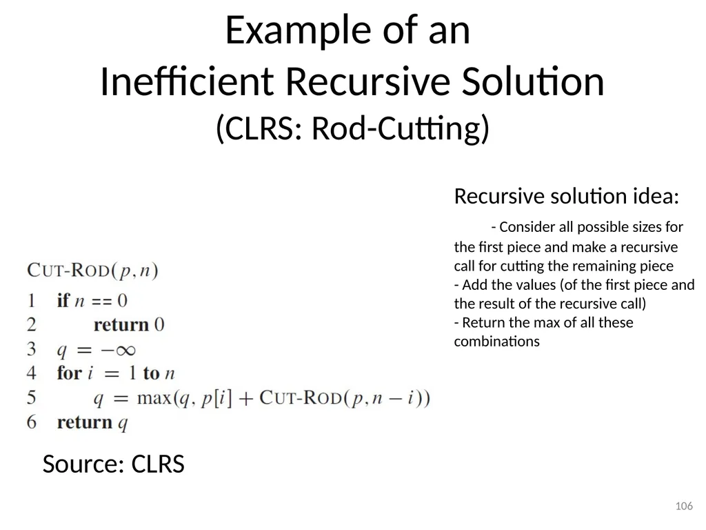
slide85. Worksheet:Inefficient Recursive Solution(CLRS: Rod-Cutting) Source: CLRS 85 Write the recurrence formula for this function: T(N) =……..<br>
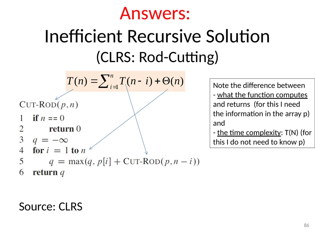
slide86. Answers: Inefficient Recursive Solution(CLRS: Rod-Cutting) Source: CLRS 86 Note the difference between
- what the function computes and returns (for this I need the information in the array p) and
- the time complexity: T(N) (for this I do not need to know p)<br>
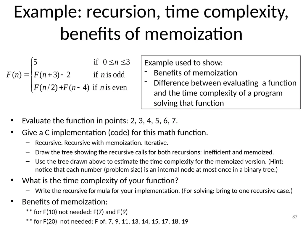
slide87. Example: recursion, time complexity,benefits of memoization Evaluate the function in points: 2, 3, 4, 5, 6, 7.
Give a C implementation (code) for this math function.
Recursive. Recursive with memoization. Iterative.
Draw the tree showing the recursive calls for both recursions: inefficient and memoized.
Use the tree drawn above to estimate the time complexity for the memoized version. (Hint: notice that each number (problem size) is an internal node at most once in a binary tree.)
What is the time complexity of your function?
Write the recursive formula for your implementation. (For solving: bring to one recursive case.)
Benefits of memoization:
** for F(10) not needed: F(7) and F(9)
** for F(20) not needed: F of: 7, 9, 11, 13, 14, 15, 17, 18, 19 87 Example used to show:
Benefits of memoization
Difference between evaluating a function and the time complexity of a program solving that function<br>
slide88. Worksheet int foo(int n){
if (n <= 1) return 3;
if (n%2 == 1)
return foo(n-1);
else
return foo(n/2)+10;
}
Math definition => code => recurrence formula => Θ
Recursive inefficient => memoized 88<br>
slide89. Answer int foo(int n){
if (n <= 1) return 3;
if (n%2 == 1)
return foo(n-1);
else
return foo(n/2)+10;
} 89 Note that in this case it is a coincidence that the recurrence formulas, T(n), for the time complexity are similar to what the function computes (and the math definition).
Typically they are different. Even here you can see the difference in the case when n is odd: the +c in the T(n) formula.<br>
slide90. Answer int foo(int n){
if (n <= 1) return 3;
if (n%2 == 1)
return 5*foo(n-1);
else
return foo(n/2)+10;
} 90 Note that when n is odd, we still use T(n-1) and not 5T(n-1), because still only one recursive call is made in the foo function when n is odd. (The result of that call is multiplied with 5, but that affects what the function computes, not its time complexity.) int foo(int n){
if (n <= 1) return 3;
if (n%2 == 1)
return foo(n-1)+foo(n-1);
else
return foo(n/2)+10;
} Because there are 2 actual calls to foo(n-1) we will have 2*T(n-1) in the recurrence formula.<br>
slide91. From Recursive Formula to CodeWorksheet Give a piece of code/pseudocode for which the time complexity recursive formula is:
T(N) = N*T(N-1) + n or
T(N) = N*T(N-1) + Θ(N)
Assume T(1) = c 91<br>
slide92. From Recursive Formula to CodeAnswers Give a piece of code/pseudocode for which the time complexity recursive formula is:
T(N) = N*T(N-1) + n or
T(N) = N*T(N-1) + Θ(N)
Assume T(1) = c 92 int foo(int N){
if (N <= 1) return 3;
for(int i=1; i<=N; i++)
foo(N-1);
}<br>
slide93. Compare 93 int foo1(int N){
if (N <= 1) return 3;
for(int i=1; i<=N; i++){
foo1(N-1);
}
}

T(N) = N*T(N-1) + cN int foo2(int N){
if (N <= 1) return 3;
for(int i=1; i<=N; i++){
printf("A");
}
foo2(N-1); // foo2(N-1) is not // in the loop
}

T(N) = T(N-1) + cN<br>
slide94. DP - summary Most problems that can be solved with DP have a solution that can be expressed with a cost function.
If the cost function is given the implementation is straight-forward. Implementation options:
Iterative
Recursive
Memoized
Guidelines for finding the cost function:
Express the solution to the problem as a sequence of independent choices/steps
Try to write the cost of the current problem using answers to subproblems:
You must consider the choice and the answer to the subproblem. 94<br>
slide95. Additional Problems 95<br>
slide96. Stair Climbing 96<br>
slide97. Stair Climbing Problem:
A child has to climb N steps of stairs. He can climb 1,2 or 3 steps at a time.
How many different ways are there to climb the stairs?
We count permutations as different ways, e.g.:
(3,1,3,1) is different than (3,3,1,1)
(2 jumps of 3 and 2 jumps of 1 in both cases, but in different order)
Let C(n) – number of different ways to climb n stairs.
Solution:
Hints:
What dictates the problem size (e.g. give 2 problems of different sizes).

What is the smallest problem size that you can solve? 97 149 81 44<br>
slide98. Stair Climbing Problem:
A child has to climb N steps of stairs. He can climb 1,2 or 3 steps at a time.
How many different ways are there to climb the stairs?
We count permutations as different ways, e.g.:
(3,1,3,1) is different than (3,3,1,1)
(2 jumps of 3 and 2 jumps of 1 in both cases, but in different order)
Let C(n) – number of different ways to climb n stairs.
Solution:
What is the last jump he can do before he reaches the top?
1,2 or 3 => C(n) = C(n-1) + C(n-2) + C(n-3)
Set-up base cases
C(0) = 1 (stays in place, this allows us to cover N = 1,2,3 by recursion)
C(x) = 0, for all x<0
Test that it works for the first few small n: 1,2,3,4:
C(1) = C(0) + C(-1) + C(-2) = 1 + 0 + 0 = 1
C(2) = C(1) + C(0) + C(-1) = 1 + 1 + 0 = 2 ( (1, 1) or (2) )
C(3) = C(2) + C(1) + C(0) = 2 + 1 + 1 = 4 ( (1,1,1) , (1,2), (2,1), (3) )
C(4) = C(3) + C(2) + C(1) = 4 + 2 + 1 = 7 98<br>
slide99. Stair Climbing Write code 99<br>
slide100. Stair ClimbingWorksheet 100 Count based on possible last steps. Possible ways to climb this many stairs.<br>
slide101. Stair climbing with gain 101 Solve for 17 stairs with the Gain (e.g. health points, HP,) per jump size given below. Here the only jump sizes that give gain are the ones in the table.
You can assume that other jump sizes are allowed, but they give 0 gain. That allows us to consider ALL problems size (for example a problem of size 1 is allowed: 1 step we have 0 gain.)<br>
slide102. Stair climbing with gain 102 Gain based on possible last steps.
These rows show the work needed to fill-in the answers in Sol and Picked. Solution (gain) for problems of this size. Last choice that gives the optimal solution. Gain with this jump Remaining
stairs Pick the maximum as the answer for this problem size, 6. The top table shows the details of the work from the last 3 rows of the bottom table.<br>
slide103. Stair climbing with gain - Answers 103 Gain based on possible last steps.
These rows show the work needed to fill-in the answers in Sol and Picked. Solution (gain) for problems of this size. Last choice that gives the optimal solution. Pick the maximum as the answer for this problem size, 6. The top table shows the details of the work from the last 3 rows of the bottom table.<br>
slide104. 104 104 Gain based on possible last steps.
These rows show the work needed to fill-in the answers in Sol and Picked.
In an implementation (code) you will NOT need a 2D array. Solution (gain) for problems of this size. Last choice that gives the optimal solution.<br>
slide105. Rod Cutting Problem Given:
A rod of a certain length, n.
An array of prices for rods of sizes between 1 and n.
What is the best way to cut the cod so that you make the most money out of selling it?
Optimization problem:
There are many ways to cut the rod, you want the best one. 105 CLRS image & formula<br>
slide106. Example of an Inefficient Recursive Solution(CLRS: Rod-Cutting) Source: CLRS 106 Recursive solution idea: - Consider all possible sizes for the first piece and make a recursive call for cutting the remaining piece
- Add the values (of the first piece and the result of the recursive call)
- Return the max of all these combinations<br>
slide107. Rod Cutting Problem Recursive solution:
Try cutting a first piece of all possible size and make a recursive call for cutting the remaining piece
Add the values (of the first piece and the result of the recursive call)
Return the max of all these combinations
Recursion tree
Example for n = 4
Notice how many times a recursive call is made for problems of the same size: 8 times for size 0, 4 times for size 1, 2 times for size 2
We will fix this inefficiency.
Properties of a tree for rod of size n:
Total nodes (including leaves): 2n. (proof by induction)
Total leaves: 2n-1. (proof by induction)
Number of leaves = number of different ways to cut the rod
Each path down to a leaf corresponds to a different way of cutting the rod. 107<br>
slide108. Rod Cutting Problem 3 solutions:
Recursive – inefficient (NOT Dynamic Programming (DP) ) –
Θ(2n)
Top-down DP (Memoization) - recursive with saving the computed results
Θ(n2)
Bottom-up DP - non-recursive
Θ(n2)
Recursion tree
For plain recursion
For memoization
Also see the solution array
DP solution complexity - Θ(n2) 108 Subproblem graph
(CLRS image)<br>
slide109. Shuttle-to-Airport Problem 109<br>
slide110. Shuttle-to-Airport Problem(Dr. Bob Weems, notes07)(We may cover this at the end) 110 1 1 2 3 4 5 6 (Airport) 3 4 5 6 (Airport) 2 0 0 9 (=7+2) 7 (=4+3) U(i) – optimal cot to reach top node i
L(i) - optimal cot to reach bottom node i
U(0) = L(0) = 0
U(i) = min{U(i-1) + UD(i), L(i-1) + LD(i)+LU(i)}
L(i) = min{L(i-1) + LD(i), U(i-1) + UD(i)+UL(i)} UD(i) – Upper direct/horizontal
LD(i) – Lower direct/horizontal
UL(i) – Upper to lower (vertical)
LU(i) – Lower to upper (vertical) Time complexity : O(n)
Fill out U and L arrays
with constant local cost.<br>
slide111. Shuttle-to-Airport ProblemBrute Force Evaluate all routes that end at the top n-th point.
The top n-th and bottom n-th points will have the same value , so we will use the top n-th point as the airport.
These are really the same point (the airport). We artificially split it into two points to make the problem representation more uniform (as opposed to having it as a special case).
Any route that ends at the bottom n-th point is a duplicate of the same route ending at the top point (with the use of one of the vertical n-th arrows with cost 0). 111 A route ending at the top.
Using the gray arrow, we get the duplicate route ending at the bottom. A route ending at the bottom.
Using the gray arrow, we get the duplicate route ending at the top.<br>
slide112. Shuttle-to-Airport ProblemBrute Force: Version 1 VERSION 1: count all the ways to get to any point.

Let:
top(i) be the total number of different ways to get to the top point, i.
bottom(i) be the total number of different ways to get to the bottom point, i.
Then:
top(0) = bottom(0) = 1 (we are already at the starting point)
top(i) = bottom(i) = top(i-1) +bottom(i-1)
=> top(i) = 2*top(i-1) => top(i) = 2i.
Straight forward proof by induction that top(i) == bottom(i) and that top(i) = 2i.
=> top(n) = 2n routes
=> O(2n) complexity of brute force 112<br>
slide113. Shuttle-to-Airport ProblemBrute Force: version 2 Version 1: count representations of all different routes.
Notice that:
A horizontal arrow will always be picked (it moves us closer to the airport)
A vertical arrow may or may not be picked.
There cannot be two consecutive vertical arrows. Between any two horizontal arrows in a solution, there may be nothing, or a vertical arrow.

The difference between two routes is in the placement of vertical arrows.
Encode only the vertical movement: 1-used (either up or down), 0-not used
is encoded as: 1 0 1 1
2n routes => O(2n)
Note that the ‘reflection’ routes will lead to the n-th bottom point and that is a duplicate solution, thus ignored. 113<br>
slide114. Shuttle-to-Airport ProblemBacktracing Version 1: record choices (h - horizontal or v-vertical arrow to reach that node)
Version 2: use the cost function to see which way you came from:
If ( (U(i-1) + UD(i) ) <= (L(i-1) + LD(i)+LU(i)) )
Horizontal (upper direct arrow used)
Else
Vertical (lower to upper arrow used)
Similar for (L(i-1) + LD(i)), and (U(i-1) + UD(i)+UL(i))
Hint, if you store U and L in a 2D array as rows, you can easily switch from top to bottom by using (row+1)%2. The row value indicates: 0-top, 1-bottom
Time complexity: O(n) 114<br>
slide115. Shuttle-to-AirportBacktracing 115 Route (in reversed order, starting from 6 top):
6 top, 5 top, 5 bottom, 4 bottom, 3 bottom, 3 top, 2 top, 2 bottom, 1 bottom, start point 5 5 5 35 5 5 10 10 35 35 35 35 35 35 Airport Optimal cost: 30 Example showing that in the first path (when computing the optimal cost) we do not
know what nodes will be part of the solution. Here the top 3 nodes have costs smaller than
their bottom correspondents, but the final top cost is too large and the bottom route
becomes optimal. (5) (10) (15) (20) (10) (25) (30)<br>
slide116. Worksheet Knapsack Example 2 116<br>
slide117. Answers Knapsack Example 2 117<br>