ECE467: Natural Language Processing Recurrent

slide1. ECE467: Natural Language Processing Recurrent Neural Networks (RNNs);
Long Short-Term Memory Networks (LSTMs)<br>
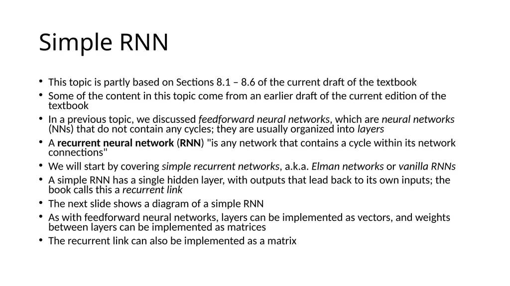
slide2. Simple RNN This topic is partly based on Sections 8.1 – 8.6 of the current draft of the textbook
Some of the content in this topic come from an earlier draft of the current edition of the textbook
In a previous topic, we discussed feedforward neural networks, which are neural networks (NNs) that do not contain any cycles; they are usually organized into layers
A recurrent neural network (RNN) "is any network that contains a cycle within its network connections"
We will start by covering simple recurrent networks, a.k.a. Elman networks or vanilla RNNs
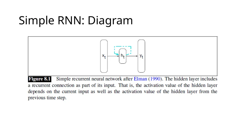
A simple RNN has a single hidden layer, with outputs that lead back to its own inputs; the book calls this a recurrent link
The next slide shows a diagram of a simple RNN
As with feedforward neural networks, layers can be implemented as vectors, and weights between layers can be implemented as matrices
The recurrent link can also be implemented as a matrix<br>
slide3. Simple RNN: Diagram<br>
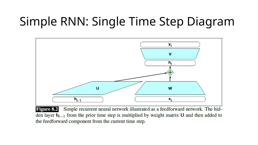
slide4. Simple RNN: Single Time Step The figure on the next slide shows what happens at a single time, or step, of the RNN as it is processing input sequentially
The caption says that the recurrent neural network is being "illustrated as a feedforward network", but I don't think of it that way
Note that ht-1 and ht refer to the same layer, but at different times or steps
Not all RNNs include an output node for every time step
Those that do can be used for sequence labeling
An example of sequence labelling in NLP is part-of-speech (POS) tagging
We covered conventional methods for this in an earlier topic
We'll discuss how a simple RNN can be for POS tagging later in this topic<br>
slide5. Simple RNN: Single Time Step Diagram<br>
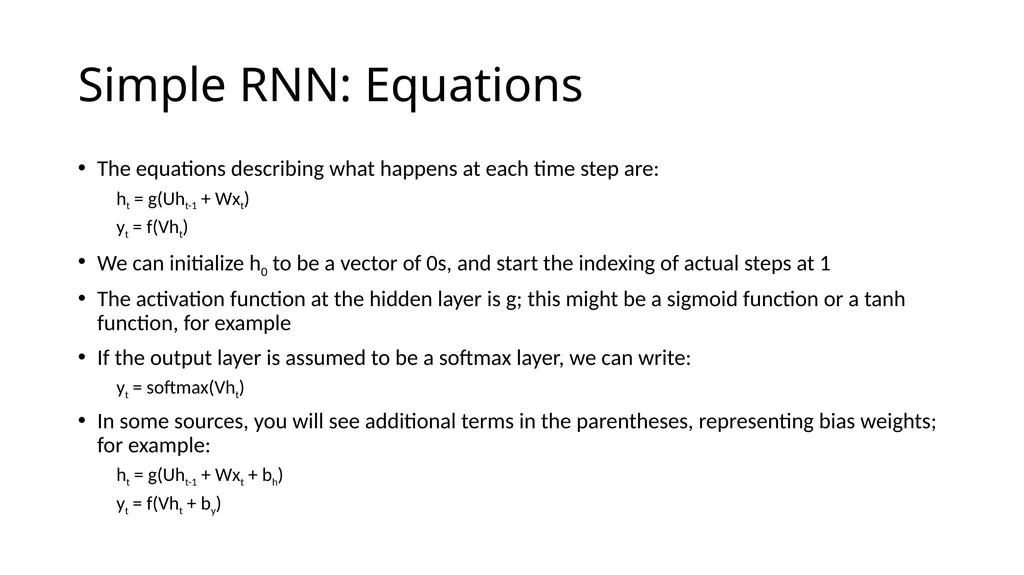
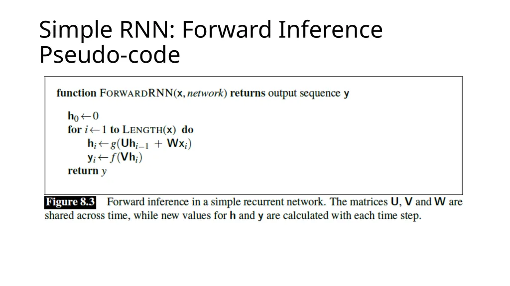
slide6. Simple RNN: Equations The equations describing what happens at each time step are:
ht = g(Uht-1 + Wxt)
yt = f(Vht)
We can initialize h0 to be a vector of 0s, and start the indexing of actual steps at 1
The activation function at the hidden layer is g; this might be a sigmoid function or a tanh function, for example
If the output layer is assumed to be a softmax layer, we can write:
yt = softmax(Vht)
In some sources, you will see additional terms in the parentheses, representing bias weights; for example:
ht = g(Uht-1 + Wxt + bh)
yt = f(Vht + by)<br>
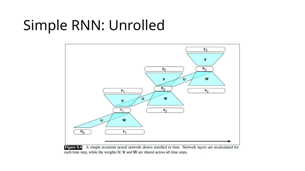
slide7. Simple RNN: Unrolling an RNN It is common to depict an RNN as unrolled
Basically, each time step (for some fixed number of time steps) is drawn separately
Each instance of the hidden layer and output layer at each of the depicted time steps is drawn separately
The next slide shows a diagram of an unrolled RNN; some things to point out are:
Depicting the unrolled RNN on a slant like this is not something I've seen in other sources
The number of depicted time steps shown in the unrolled network is arbitrary; when a simple RNN is applied to input, it keeps taking inputs until there are no more
The values at the hidden layers and output nodes are changing, but the U, W, and V matrices are not; the weights change during training, but not during forward inference
Such a diagram helps intuit how forward inference in an RNN proceeds<br>
slide8. Simple RNN: Unrolled<br>
slide9. Simple RNN: Forward Inference Forward inference, also called forward propagation, in an RNN proceeds much like with a feedforward neural network
However, with a feedforward neural network, all the input is fed to the NN at once
With an RNN, a series or sequence of inputs is fed to the NN across multiple time steps
The values of hidden nodes and the output nodes change at each time step
The values of the weights (often implemented as matrices) do not; that is, the same weights are reused at each time step
Of course, when we train an RNN, the weights will change (but we haven’t talked about how to do that yet)
The figure on the next slide shows pseudo-code for forward inference with a simple RNN<br>
slide10. Simple RNN: Forward Inference Pseudo-code<br>
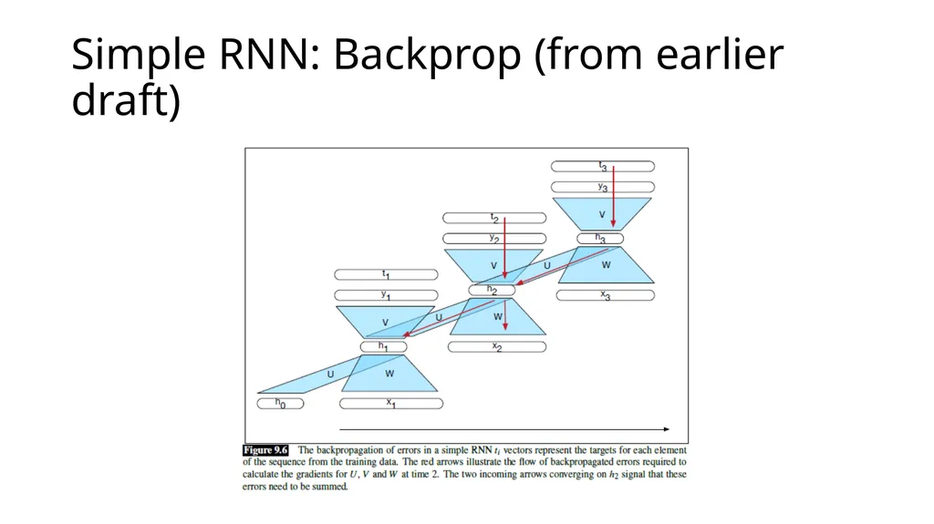
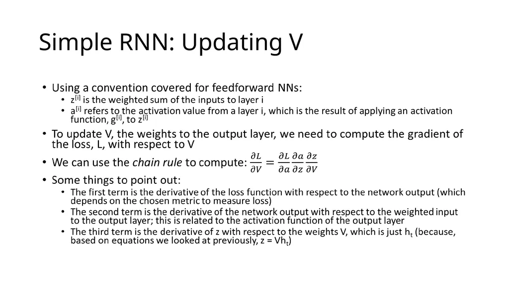
slide11. Simple RNN: Training As with feedforward neural networks, we can train a simple RNN using stochastic gradient descent (SGD) and backpropagation
Also, as with feedforward neural networks, we need a training set, and we need to define a loss function
For our simple RNN, we now have three sets of weights to update:
W represents the weights between the input layer and the hidden layer
V represents the weights between the hidden layer and the output layer
U represents the weights from the output of the hidden layer (at one time step) to the input of the hidden layer (at the next time step)
Some formulations will also include bias weights, which also need to be updated
The current draft of the textbook has dropped most of the discussion of training RNNs, but we will still discuss this in some detail
The figure on the next slide, from an earlier draft of the textbook (from October 16, 2019), helps to visualize this
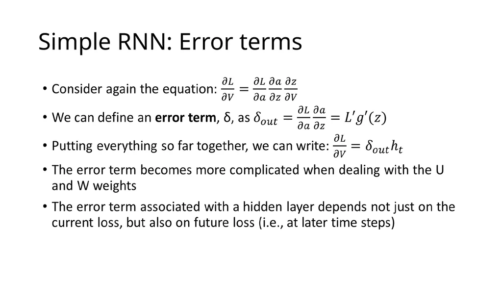
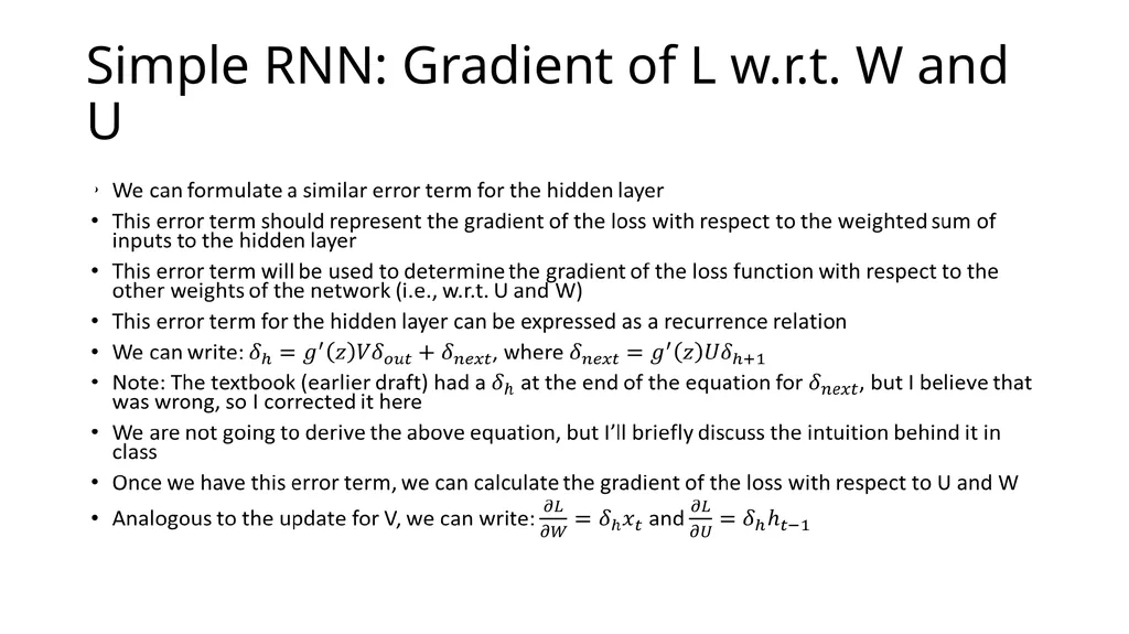
More generally, much of the information we discuss related to training RNNs over the next several slides is based on that earlier draft<br>
slide12. Simple RNN: Backprop (from earlier draft)<br>
slide13. Simple RNN: Updating V<br>
slide14. Simple RNN: Error terms<br>
slide15. Simple RNN: Gradient of L w.r.t. W and U<br>
slide16. Simple RNN: Two-pass Weight Training The book (current draft) talks about a "two-pass algorithm for training weights in RNNs"
First, we perform forward inference, computing all the h and y values at every time step
Second, we "process the sequence in reverse", computing the required error terms and gradients
The book does not specify when weights are actually updated
My understanding, based on other sources, is that the gradients during the backward pass are accumulated, and the sum is used to adjust the weights
This type of training process is sometimes called backpropagation through time<br>
slide17. Simple RNN: Language Model Simple RNNs can be used as recurrent neural language models
The previous hidden state and the current word are used to calculate the current hidden state
The current hidden state is fed to a softmax layer, which creates a probability distribution used to predict the next word
As with other language models (e.g., N-grams or feedforward NNs), we combine probabilities to evaluate the model
In practice, log probabilities or perplexity is used
Unlike the previous language models we considered, RNNs are not limited to a fixed number of prior words when predicting the next word
That is, all the words in the sequence so far can affect the prediction of the next word, in theory
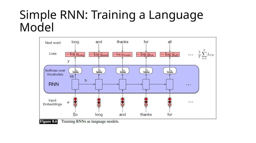
The diagram on the next slide helps to explain how to train a simple RNN to behave as a language model, assuming that we are using a cross-entropy loss function<br>
slide18. Simple RNN: Training a Language Model<br>
slide19. Simple RNN: Autoregressive Generation A related task is autoregressive generation, which automatically generates random text
In a previous topic, we saw the results of using N-grams for this type of natural language generation, when trained on Shakespeare or the Wall Street Journal
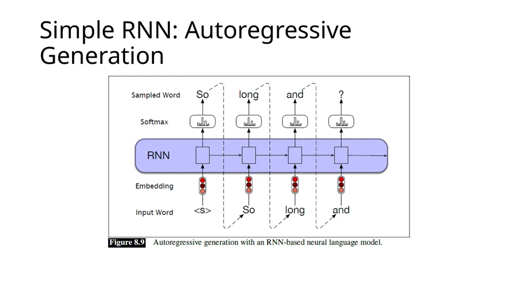
Once a simple RNN is trained as a language model, we can apply the RNN to generate random text; the probabilities of each possible next word are used to randomly choose a word
The diagram on the next slide shows how to apply the simple RNN for autoregressive generation; some things to point out are:
The inputs are pre-trained word embeddings
The <s> is a beginning of sentence marker, which has its own embedding
The hidden state can be interpreted as being a semantic representation of all content that has been processed so far
The output of the softmax is not used to predict the most likely word, but rather as a probability distribution from which to sample the next word
The processing ends either after a fixed number of tokens, or when an end of sentence marker, </s>, is produced
Earlier drafts of the book referred autoregressive generation as an "entertaining exercise"
However, as recognized in the current draft, this sort of generation is crucial to modern NLP applications, such as machine translation, summarization, question answering, and chatbots
We will discuss some of these applications later in the course<br>
slide20. Simple RNN: Autoregressive Generation<br>
slide21. Simple RNN: Sequence labelling Sequence labeling refers to any task that involves categorizing every item in a sequence
One example which we talked about during a previous topic is is part-of-speech (POS) tagging
Conventional approaches for POS tagging included hidden Markov models and maximum entropy Markov models (we no long cover these in this course)
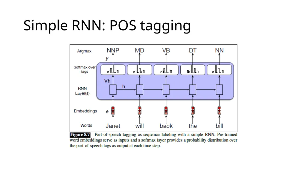
The figure on the next slide shows how a simple RNN could be applied to POS tagging
Note that each decision would be affected by all the words seen so far
The textbook does not address how well a simple RNN would perform for POS tagging (but probably not very well)
State-of-the-art POS tagging uses more complex variations of RNNs such as LSTMs (we will cover this soon) or transformers (a future topic)<br>
slide22. Simple RNN: POS tagging<br>
slide23. Simple RNN: Named Entity Recognition Another important sequence labelling task in NLP is named entity recognition (NER)
NER involves detecting spans of text representing names of people, places, organization, etc.
It can also include additional concepts such as times and dates, or domain-specific entities such as diseases, symptoms, medications, etc.
NER is sometimes the first phase of other tasks, such as information extraction
NER system are typically trained using supervised machine learning
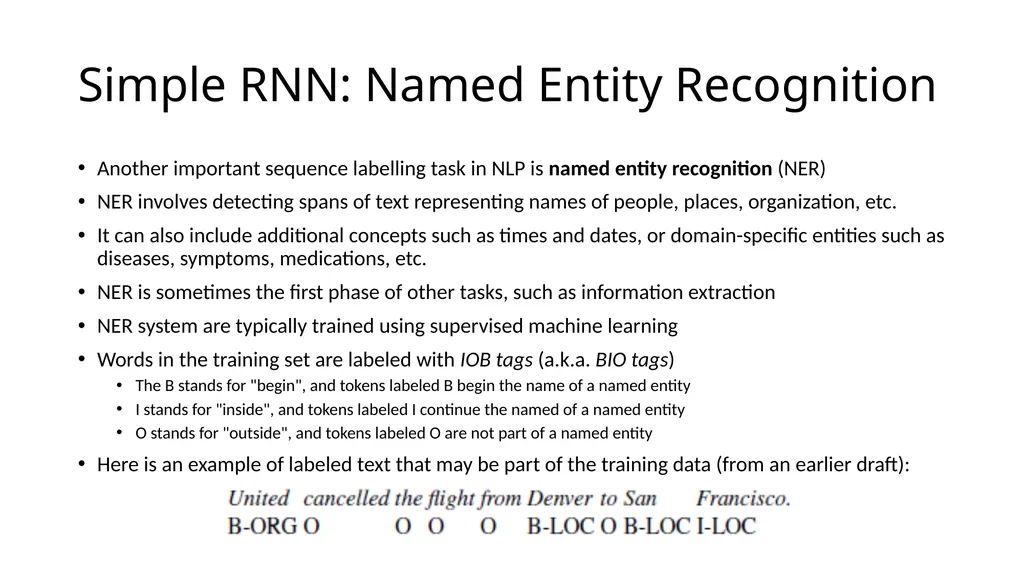
Words in the training set are labeled with IOB tags (a.k.a. BIO tags)
The B stands for "begin", and tokens labeled B begin the name of a named entity
I stands for "inside", and tokens labeled I continue the named of a named entity
O stands for "outside", and tokens labeled O are not part of a named entity
Here is an example of labeled text that may be part of the training data (from an earlier draft):<br>
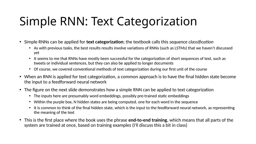
slide24. Simple RNN: Text Categorization Simple RNNs can be applied for text categorization; the textbook calls this sequence classification
As with previous tasks, the best results results involve variations of RNNs (such as LSTMs) that we haven’t discussed yet
It seems to me that RNNs have mostly been successful for the categorization of short sequences of text, such as tweets or individual sentences, but they can also be applied to longer documents
Of course, we covered conventional methods of text categorization during our first unit of the course
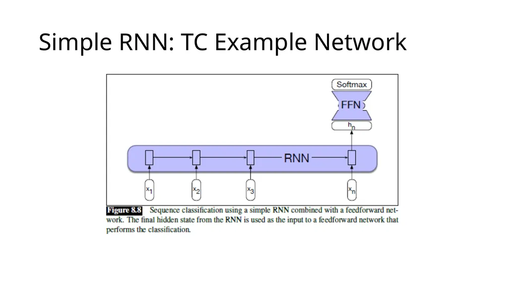
When an RNN is applied for text categorization, a common approach is to have the final hidden state become the input to a feedforward neural network
The figure on the next slide demonstrates how a simple RNN can be applied to text categorization
The inputs here are presumably word embeddings, possibly pre-trained static embeddings
Within the purple box, N hidden states are being computed, one for each word in the sequence
It is common to think of the final hidden state, which is the input to the feedforward neural network, as representing the meaning of the text
This is the first place where the book uses the phrase end-to-end training, which means that all parts of the system are trained at once, based on training examples (I'll discuss this a bit in class)<br>
slide25. Simple RNN: TC Example Network<br>
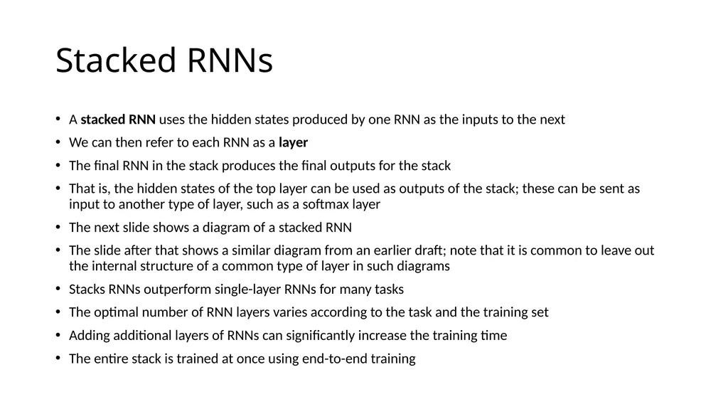
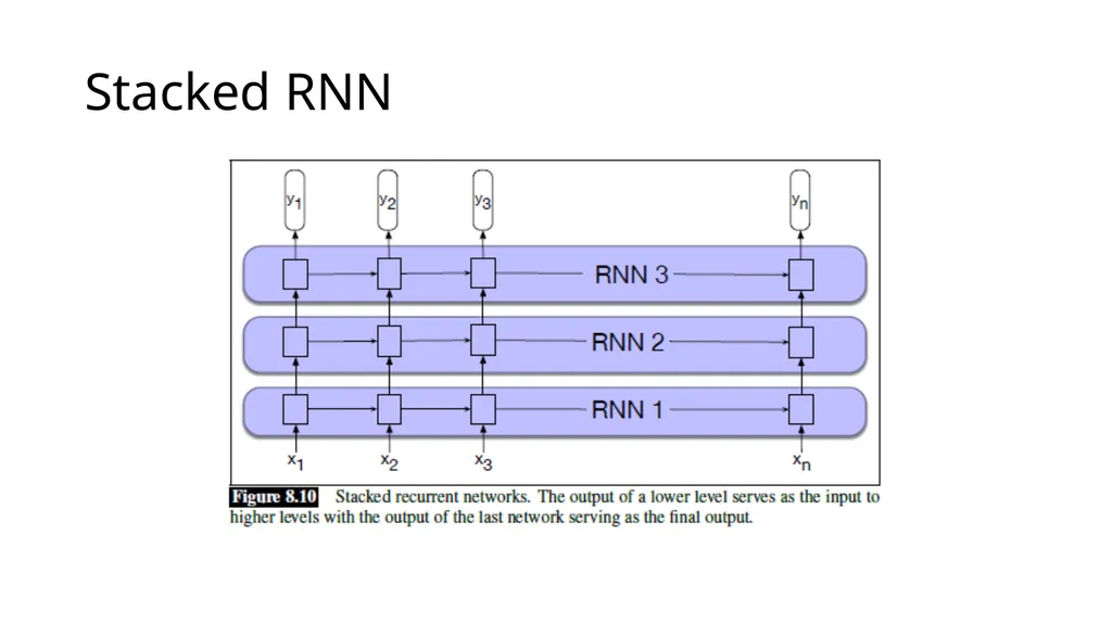
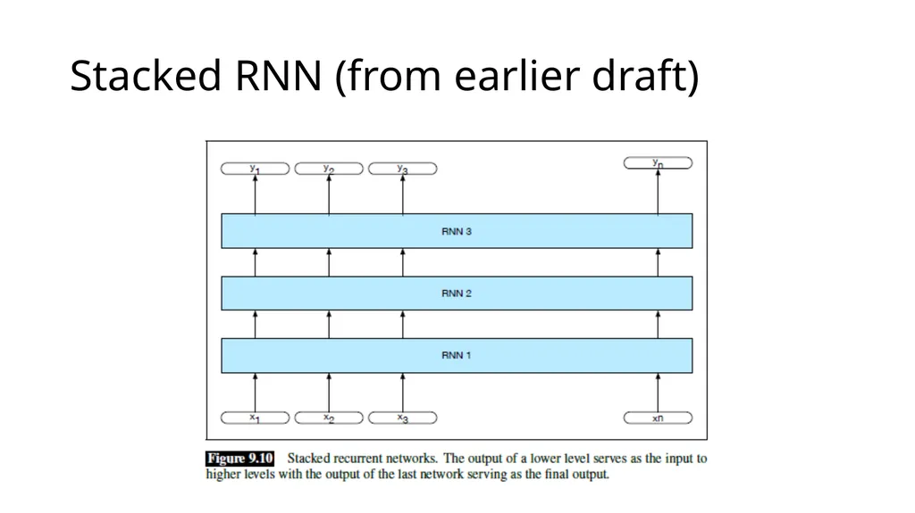
slide26. Stacked RNNs A stacked RNN uses the hidden states produced by one RNN as the inputs to the next
We can then refer to each RNN as a layer
The final RNN in the stack produces the final outputs for the stack
That is, the hidden states of the top layer can be used as outputs of the stack; these can be sent as input to another type of layer, such as a softmax layer
The next slide shows a diagram of a stacked RNN
The slide after that shows a similar diagram from an earlier draft; note that it is common to leave out the internal structure of a common type of layer in such diagrams
Stacks RNNs outperform single-layer RNNs for many tasks
The optimal number of RNN layers varies according to the task and the training set
Adding additional layers of RNNs can significantly increase the training time
The entire stack is trained at once using end-to-end training<br>
slide27. Stacked RNN<br>
slide28. Stacked RNN (from earlier draft)<br>
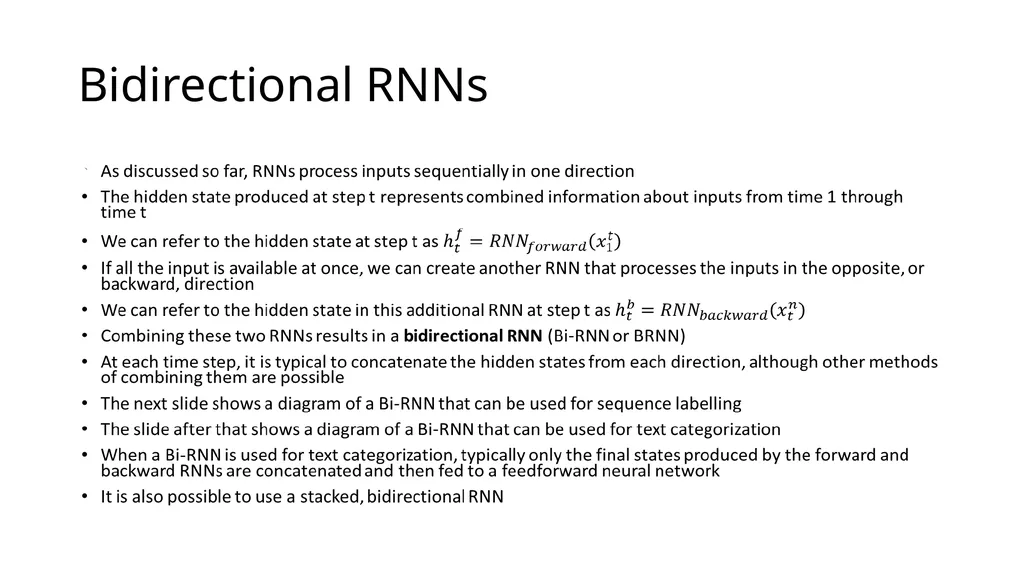
slide29. Bidirectional RNNs<br>
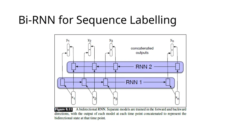
slide30. Bi-RNN for Sequence Labelling<br>
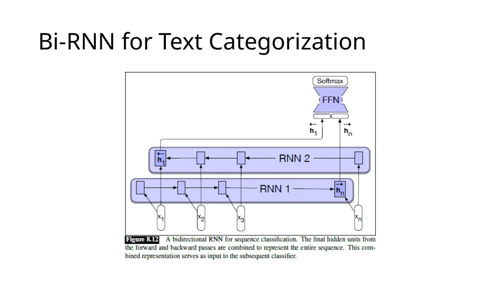
slide31. Bi-RNN for Text Categorization<br>
slide32. The Vanishing Gradient Problem All variations of RNNs discussed so far still have problems that hinder their performance for most NLP tasks
During backpropagation, for each layer or time step that error is backpropagated, there is a multiplication taking place
Typically, these multiplications reduce the gradients
That is, the further back we go, the less significant layers or states seem to be, in terms of how they affect the measured loss during training
This leads to the vanishing gradient problem; it affects all deep neural network architectures, not only RNNs
For other sorts of architectures (e.g., CNNs and feedforward NNs), rectified linear units (ReLUs) mitigate the problem to some extent
ReLUs are not typically used for RNNs (I have read various speculation about why they don't work well for RNNs, but I have not found any particularly convincing)
I add:
Sometimes, multiplications increase the gradients, leading to what is then called the exploding gradient problem (not mentioned in our textbook)
It turns out that simply capping the gradient to some fixed maximum provides an adequate solution to the exploding gradient problem
Unfortunately, there is no such simple solution for the vanishing gradient problem<br>
slide33. Non-local Context Without any solution to mitigate the vanishing gradient problem, only very local context winds up being significant
I have read that, for NLP tasks, hidden states in a simple RNN are only significantly influenced by the previous two or three words
Sometimes that is not enough
Consider: "The flights the airline was cancelling were full."
In order to know that "were" is the appropriate word, we need to recognize that the subject of the sentence, "flights", is plural
Note that the only other noun in between, "airline", is singular<br>
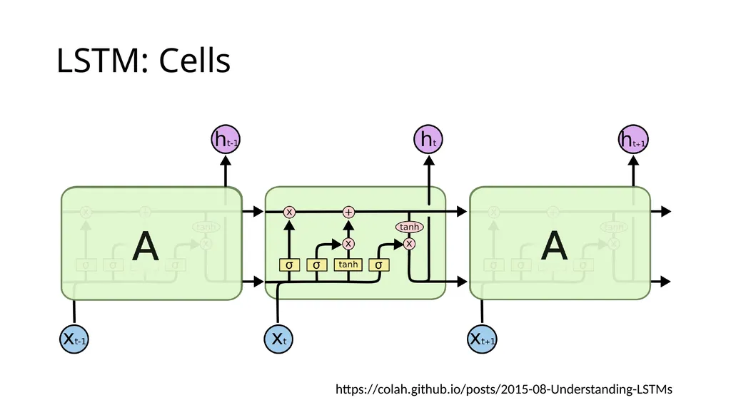
slide34. Long Short-Term Memory Units Long short-term memory (LSTM) networks provide one solution for mitigating the vanishing gradient problem
In addition to the on-line draft of the textbook, I have also relied on this blog post for my slides on LSTMs:
https://colah.github.io/posts/2015-08-Understanding-LSTMs
Often, the network as a whole, or each layer of a stacked network, is referred to as an LSTM
It is common to depict LSTMs graphically in terms of cells (our textbook calls them units, but this is not common)
Such depictions show the LSTM unrolled; the cell is the component of the architecture that repeats
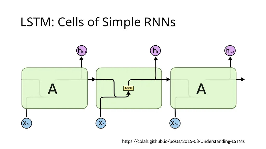
We can also depict simple RNNs as cells, for a quick comparison
The next slide shows a diagram of an unrolled simple RNN in terms of cells, assuming a tanh activation function (from the LSTM blog)
The slide after that shows a diagram of an LSTM in terms of cells (from the LSTM blog); note that the cells are more complex<br>
slide35. LSTM: Cells of Simple RNNs https://colah.github.io/posts/2015-08-Understanding-LSTMs<br>
slide36. LSTM: Cells https://colah.github.io/posts/2015-08-Understanding-LSTMs<br>
slide37. LSTM: Input and Output of Cells LSTM cells have two sets of values that are passed between cells (really being passed as feedback between one time step and the next)
One set of values (the one on top in the figure) is typically referred to as the cell state (our textbook refers to it as the cell's context)
The other set of values is the cell's hidden state
Our textbook refers to these two sets of values as separate layers of an LSTM network, but this does not seem to be common usage<br>
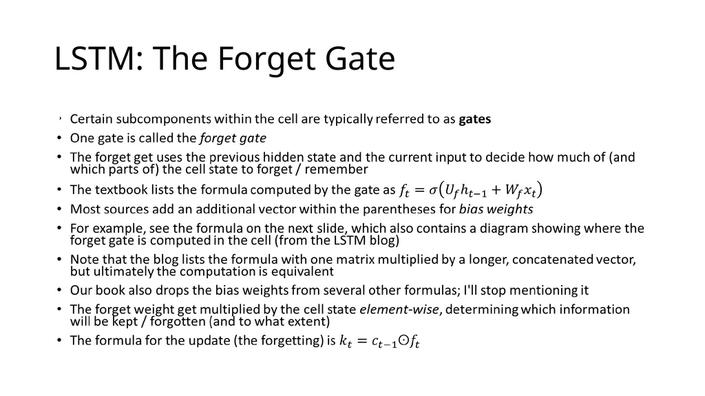
slide38. LSTM: The Forget Gate<br>
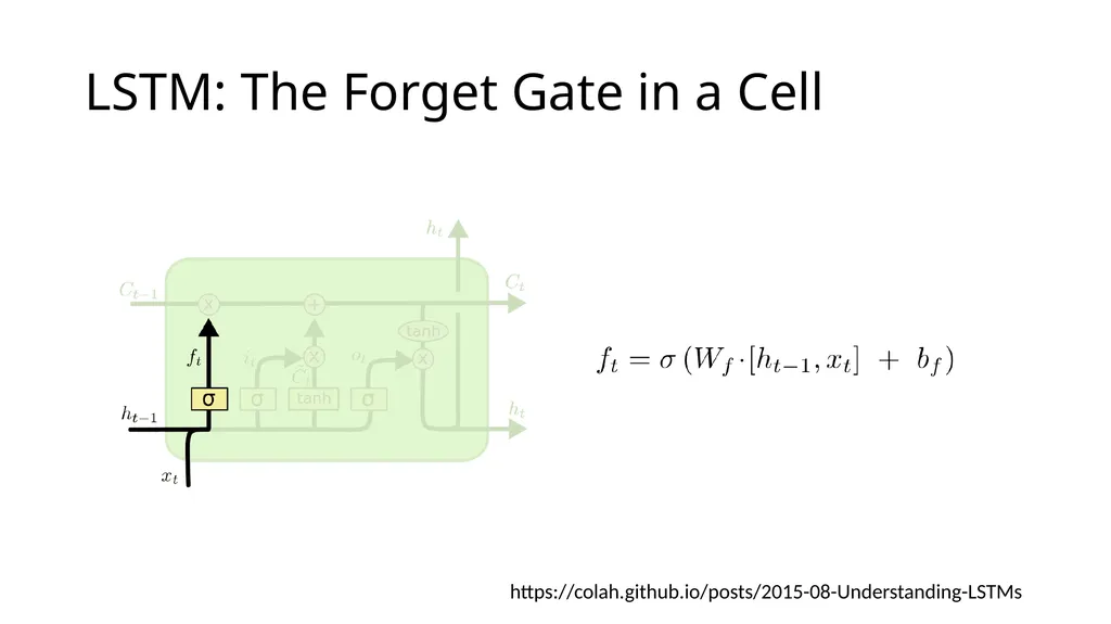
slide39. LSTM: The Forget Gate in a Cell https://colah.github.io/posts/2015-08-Understanding-LSTMs<br>
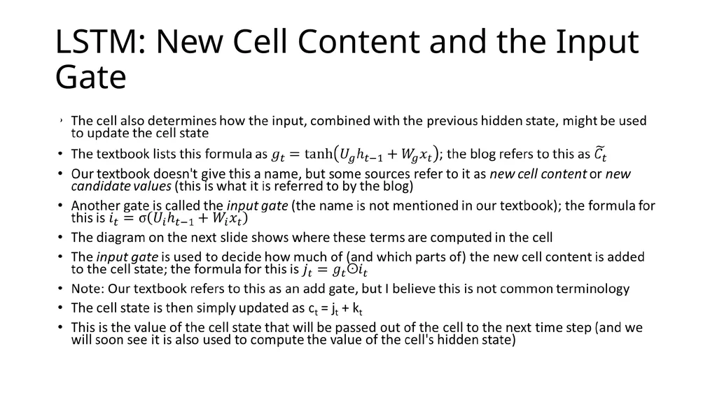
slide40. LSTM: New Cell Content and the Input Gate<br>
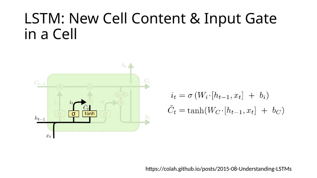
slide41. LSTM: New Cell Content & Input Gate in a Cell https://colah.github.io/posts/2015-08-Understanding-LSTMs<br>
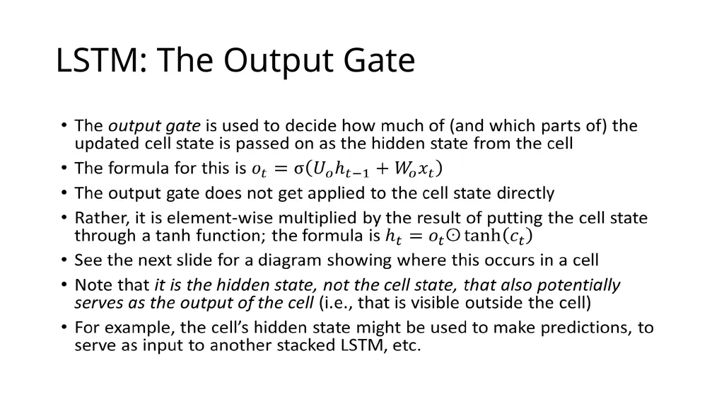
slide42. LSTM: The Output Gate<br>
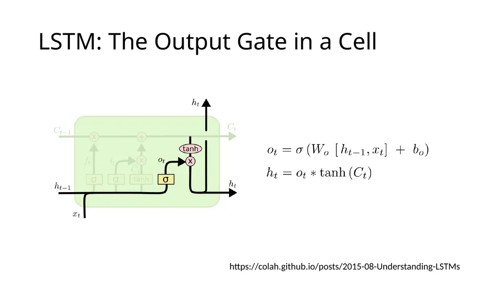
slide43. LSTM: The Output Gate in a Cell https://colah.github.io/posts/2015-08-Understanding-LSTMs<br>
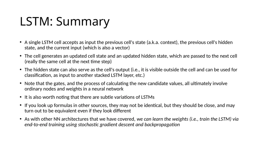
slide44. LSTM: Summary A single LSTM cell accepts as input the previous cell's state (a.k.a. context), the previous cell's hidden state, and the current input (which is also a vector)
The cell generates an updated cell state and an updated hidden state, which are passed to the next cell (really the same cell at the next time step)
The hidden state can also serve as the cell's output (i.e., it is visible outside the cell and can be used for classification, as input to another stacked LSTM layer, etc.)
Note that the gates, and the process of calculating the new candidate values, all ultimately involve ordinary nodes and weights in a neural network
It is also worth noting that there are subtle variations of LSTMs
If you look up formulas in other sources, they may not be identical, but they should be close, and may turn out to be equivalent even if they look different
As with other NN architectures that we have covered, we can learn the weights (i.e., train the LSTM) via end-to-end training using stochastic gradient descent and backpropagation<br>
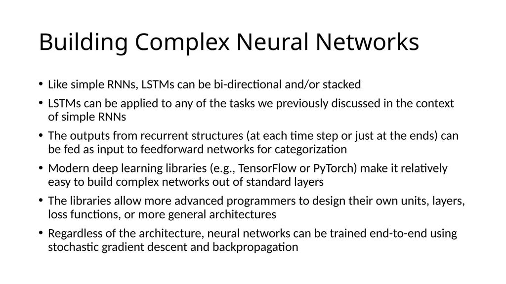
slide45. Building Complex Neural Networks Like simple RNNs, LSTMs can be bi-directional and/or stacked
LSTMs can be applied to any of the tasks we previously discussed in the context of simple RNNs
The outputs from recurrent structures (at each time step or just at the ends) can be fed as input to feedforward networks for categorization
Modern deep learning libraries (e.g., TensorFlow or PyTorch) make it relatively easy to build complex networks out of standard layers
The libraries allow more advanced programmers to design their own units, layers, loss functions, or more general architectures
Regardless of the architecture, neural networks can be trained end-to-end using stochastic gradient descent and backpropagation<br>