
Econometrics, Machine Learning Gregory M Duncan



Description: Econometrics, Machine Learning Gregory M Duncan Amazon.com University of Washington and All that stuff Introduction Vast data available today hundreds of billions of observations and millions of features A 100,000,000,000 x 1,500,000
Related Topics
Download Presentation
"Econometrics, Machine Learning Gregory M Duncan" is the property of its rightful owner. Permission is granted to download and print the materials on this website for personal, non-commercial use only, and to display it on your personal computer provided you do not modify the materials and that you retain all copyright notices contained in the materials. By downloading content from our website, you accept the terms of this agreement.
Presentation Transcript
slide1. Econometrics, Machine Learning Gregory M Duncan
Amazon.com
University of Washington and All that stuff<br>
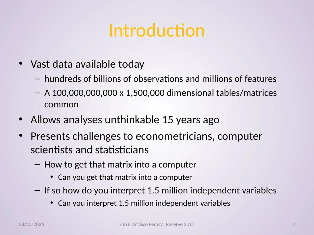
slide2. Introduction Vast data available today
hundreds of billions of observations and millions of features
A 100,000,000,000 x 1,500,000 dimensional tables/matrices common
Allows analyses unthinkable 15 years ago
Presents challenges to econometricians, computer scientists and statisticians
How to get that matrix into a computer
Can you get that matrix into a computer
If so how do you interpret 1.5 million independent variables
Can you interpret 1.5 million independent variables 11/3/2017 San Francisco Federal Reserve 2017 2<br>
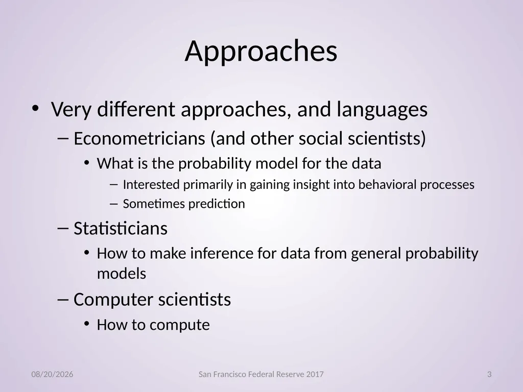
slide3. Approaches Very different approaches, and languages
Econometricians (and other social scientists)
What is the probability model for the data
Interested primarily in gaining insight into behavioral processes
Sometimes prediction
Statisticians
How to make inference for data from general probability models
Computer scientists
How to compute 11/3/2017 San Francisco Federal Reserve 2017 3<br>
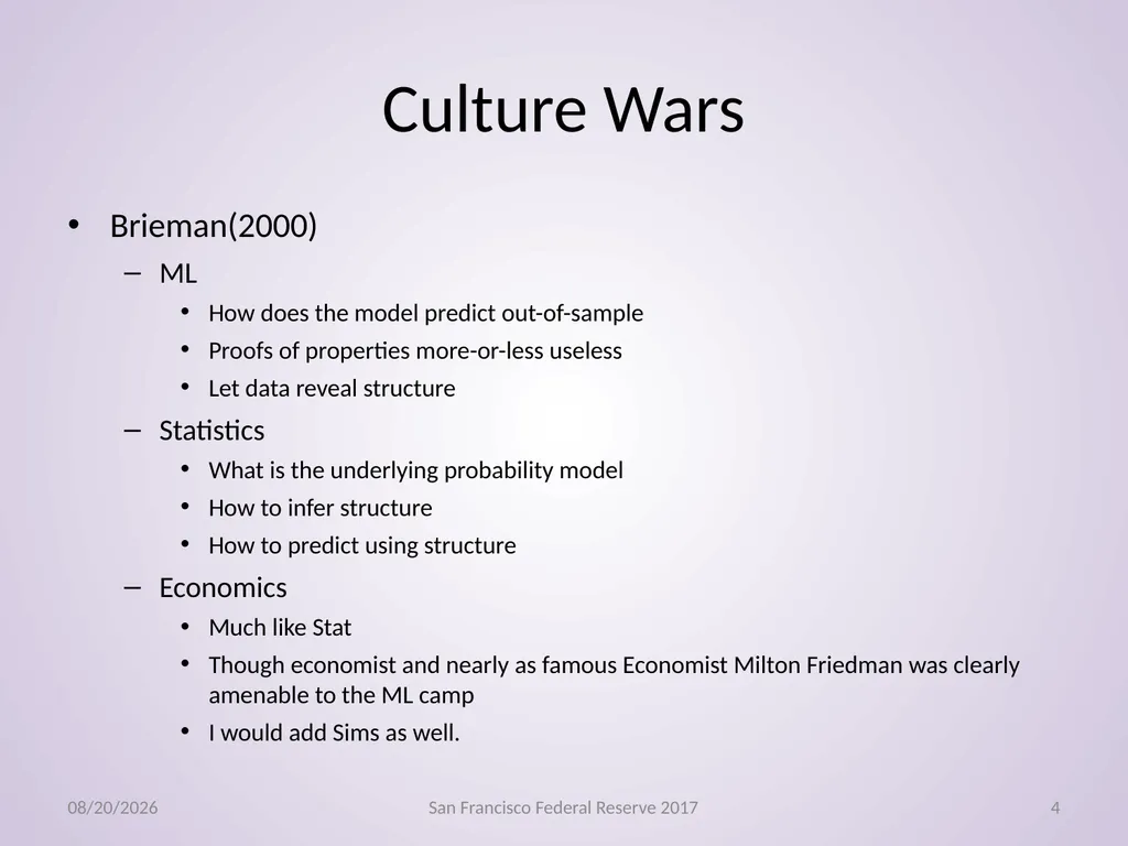
slide4. Culture Wars Brieman(2000)
ML
How does the model predict out-of-sample
Proofs of properties more-or-less useless
Let data reveal structure
Statistics
What is the underlying probability model
How to infer structure
How to predict using structure
Economics
Much like Stat
Though economist and nearly as famous Economist Milton Friedman was clearly amenable to the ML camp
I would add Sims as well. 11/3/2017 San Francisco Federal Reserve 2017 4<br>
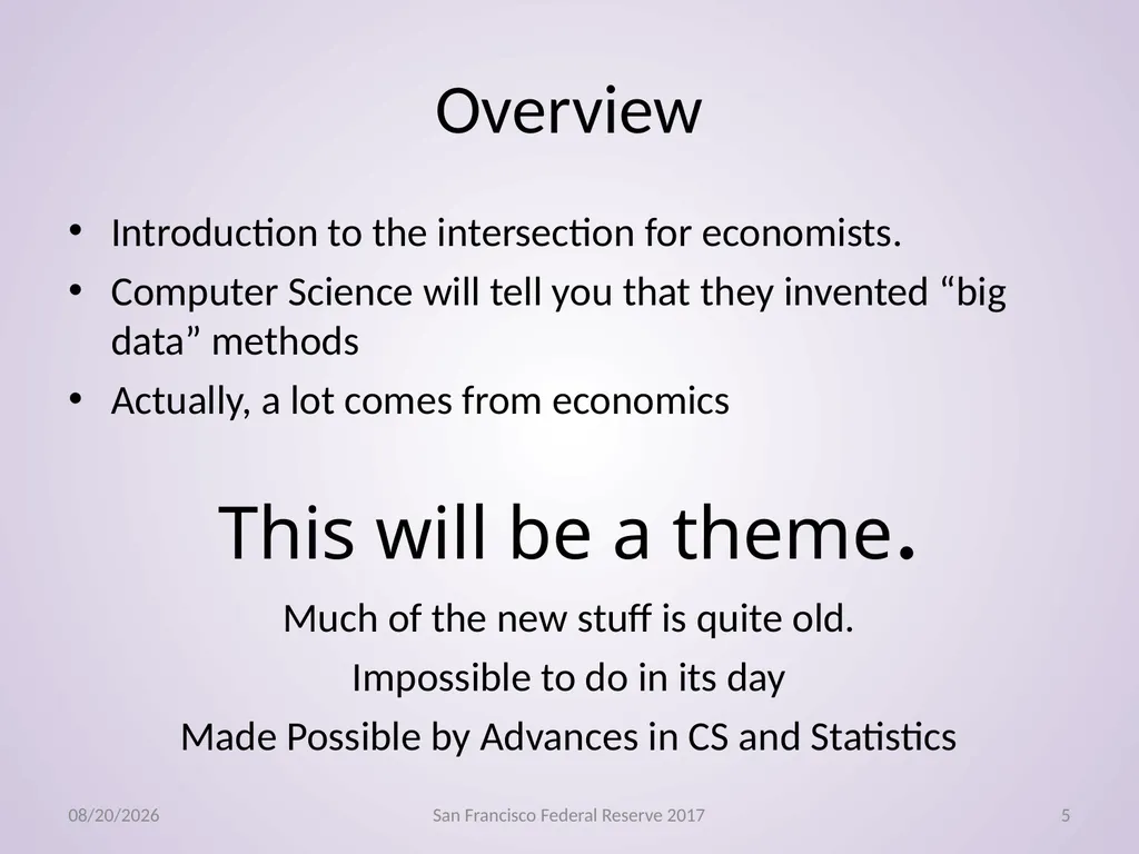
slide5. Overview Introduction to the intersection for economists.
Computer Science will tell you that they invented “big data” methods
Actually, a lot comes from economics
This will be a theme.
Much of the new stuff is quite old.
Impossible to do in its day
Made Possible by Advances in CS and Statistics 11/3/2017 San Francisco Federal Reserve 2017 5<br>
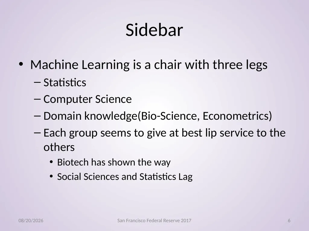
slide6. Sidebar Machine Learning is a chair with three legs
Statistics
Computer Science
Domain knowledge(Bio-Science, Econometrics)
Each group seems to give at best lip service to the others
Biotech has shown the way
Social Sciences and Statistics Lag 11/3/2017 San Francisco Federal Reserve 2017 6<br>
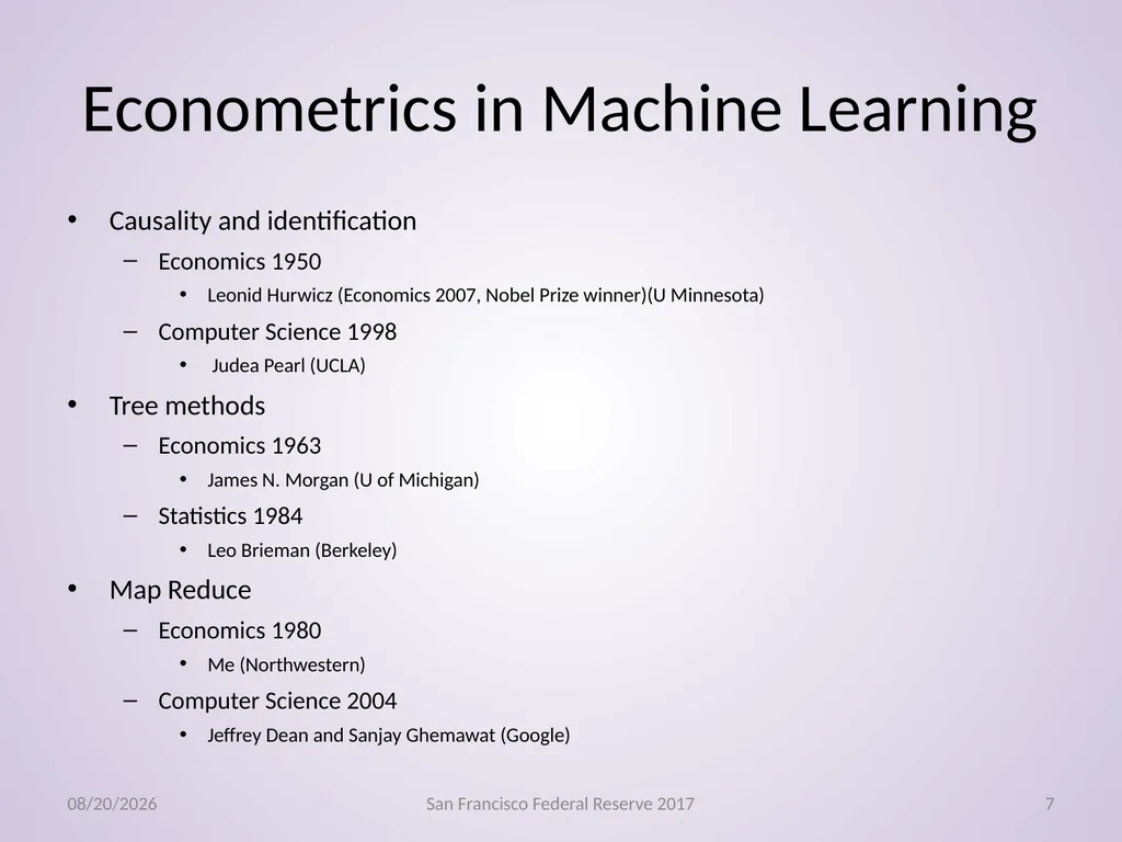
slide7. Econometrics in Machine Learning Causality and identification
Economics 1950
Leonid Hurwicz (Economics 2007, Nobel Prize winner)(U Minnesota)
Computer Science 1998
Judea Pearl (UCLA)
Tree methods
Economics 1963
James N. Morgan (U of Michigan)
Statistics 1984
Leo Brieman (Berkeley)
Map Reduce
Economics 1980
Me (Northwestern)
Computer Science 2004
Jeffrey Dean and Sanjay Ghemawat (Google) 11/3/2017 San Francisco Federal Reserve 2017 7<br>
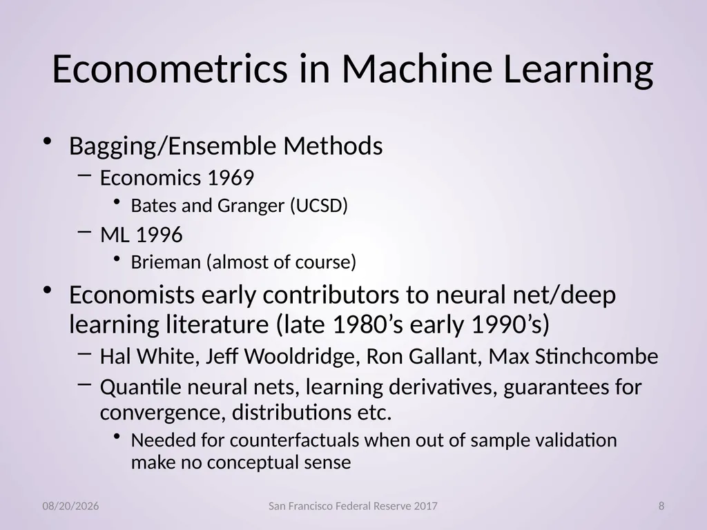
slide8. Econometrics in Machine Learning Bagging/Ensemble Methods
Economics 1969
Bates and Granger (UCSD)
ML 1996
Brieman (almost of course)
Economists early contributors to neural net/deep learning literature (late 1980’s early 1990’s)
Hal White, Jeff Wooldridge, Ron Gallant, Max Stinchcombe
Quantile neural nets, learning derivatives, guarantees for convergence, distributions etc.
Needed for counterfactuals when out of sample validation make no conceptual sense 11/3/2017 San Francisco Federal Reserve 2017 8<br>
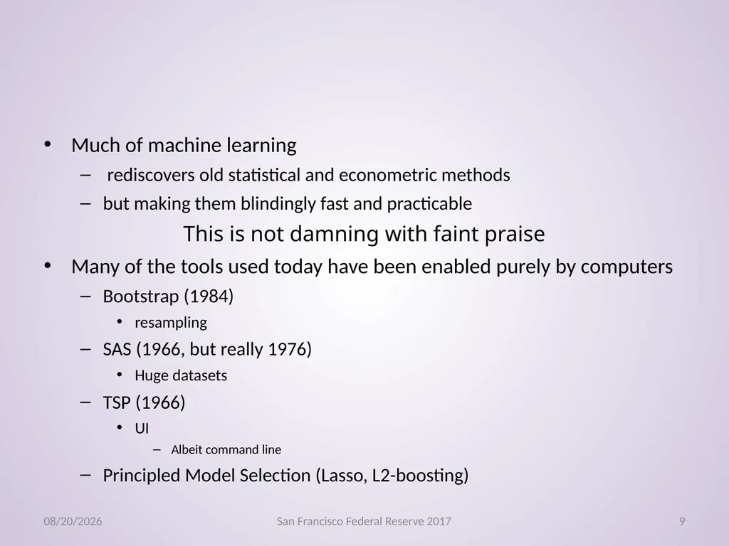
slide9. Much of machine learning
rediscovers old statistical and econometric methods
but making them blindingly fast and practicable
This is not damning with faint praise
Many of the tools used today have been enabled purely by computers
Bootstrap (1984)
resampling
SAS (1966, but really 1976)
Huge datasets
TSP (1966)
UI
Albeit command line
Principled Model Selection (Lasso, L2-boosting) 11/3/2017 San Francisco Federal Reserve 2017 9<br>
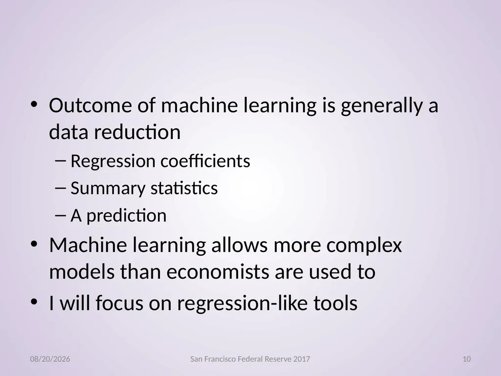
slide10. Outcome of machine learning is generally a data reduction
Regression coefficients
Summary statistics
A prediction
Machine learning allows more complex models than economists are used to
I will focus on regression-like tools 11/3/2017 San Francisco Federal Reserve 2017 10<br>
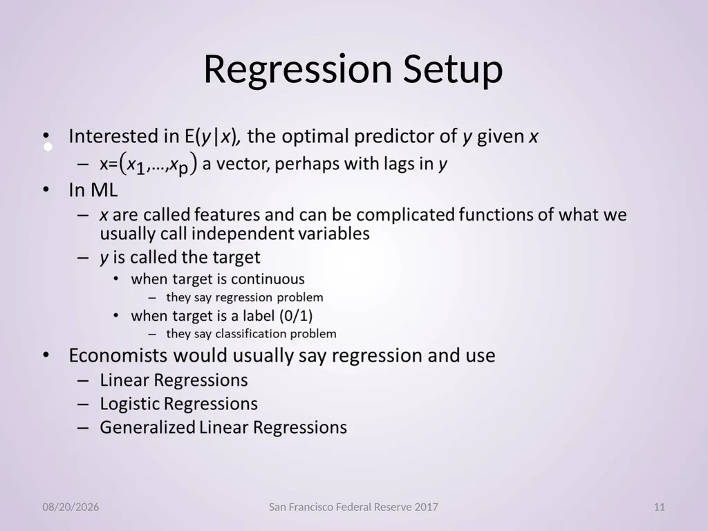
slide11. Regression Setup 11/3/2017 San Francisco Federal Reserve 2017 11<br>
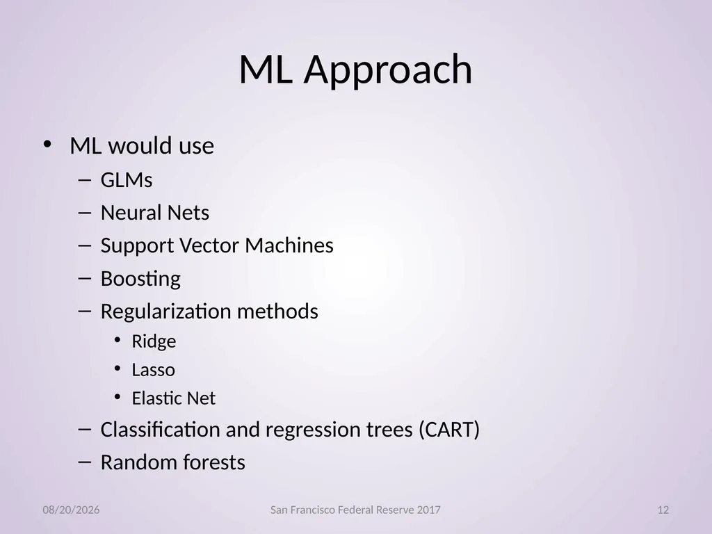
slide12. ML Approach ML would use
GLMs
Neural Nets
Support Vector Machines
Boosting
Regularization methods
Ridge
Lasso
Elastic Net
Classification and regression trees (CART)
Random forests 11/3/2017 San Francisco Federal Reserve 2017 12<br>
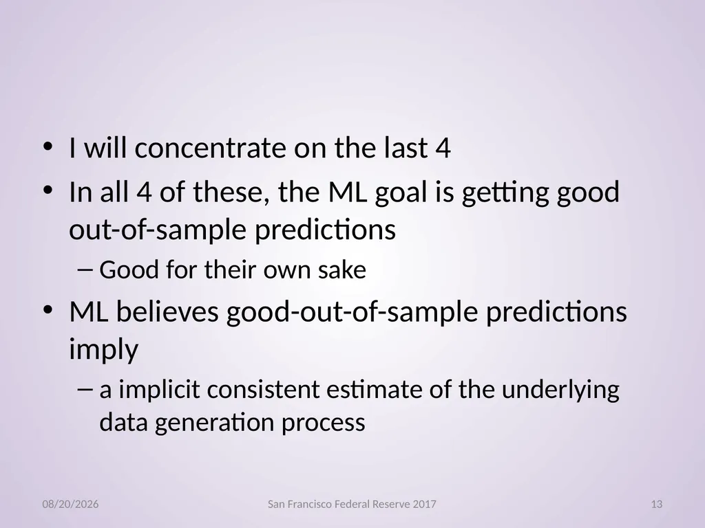
slide13. I will concentrate on the last 4
In all 4 of these, the ML goal is getting good out-of-sample predictions
Good for their own sake
ML believes good-out-of-sample predictions imply
a implicit consistent estimate of the underlying data generation process 11/3/2017 San Francisco Federal Reserve 2017 13<br>
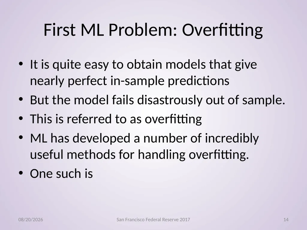
slide14. First ML Problem: Overfitting It is quite easy to obtain models that give nearly perfect in-sample predictions
But the model fails disastrously out of sample.
This is referred to as overfitting
ML has developed a number of incredibly useful methods for handling overfitting.
One such is 11/3/2017 San Francisco Federal Reserve 2017 14<br>
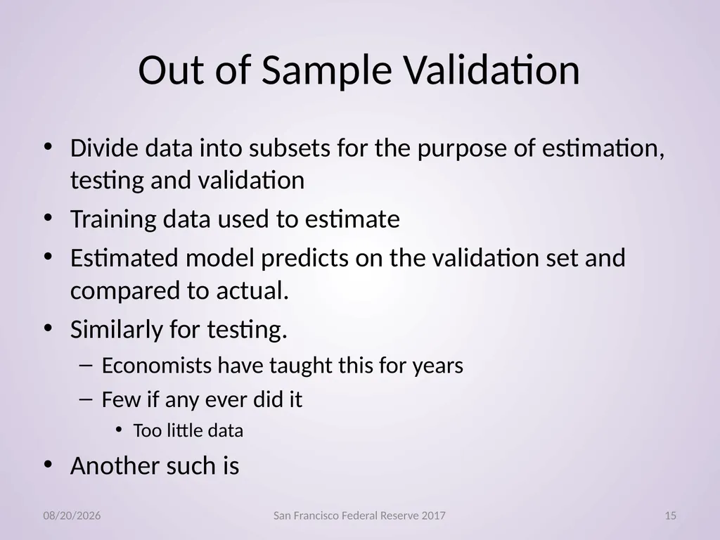
slide15. Out of Sample Validation Divide data into subsets for the purpose of estimation, testing and validation
Training data used to estimate
Estimated model predicts on the validation set and compared to actual.
Similarly for testing.
Economists have taught this for years
Few if any ever did it
Too little data
Another such is 11/3/2017 San Francisco Federal Reserve 2017 15<br>
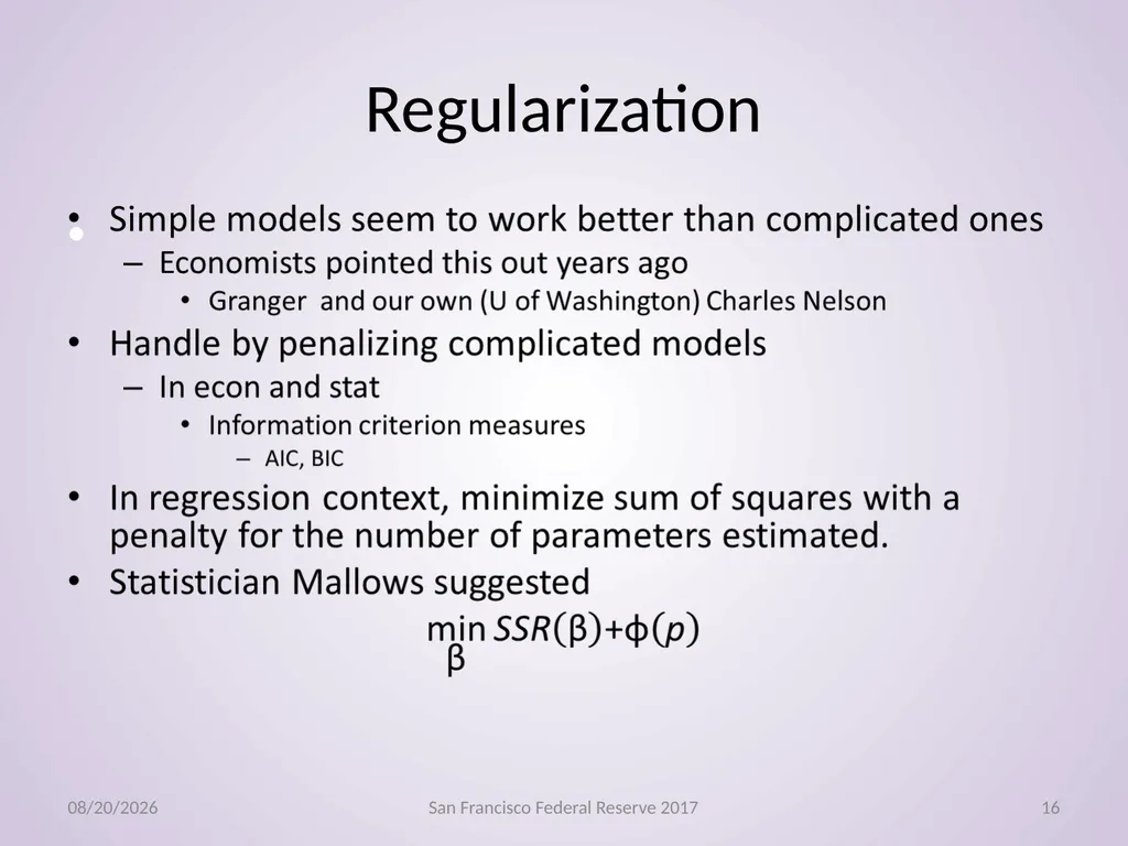
slide16. Regularization 11/3/2017 San Francisco Federal Reserve 2017 16<br>
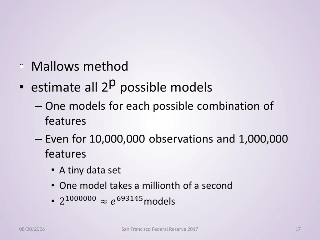
slide17. 11/3/2017 San Francisco Federal Reserve 2017 17<br>
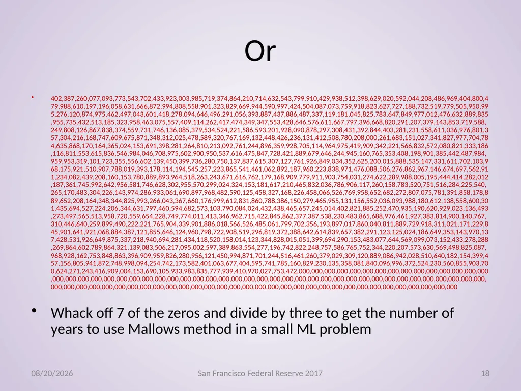
slide18. Or 402,387,260,077,093,773,543,702,433,923,003,985,719,374,864,210,714,632,543,799,910,429,938,512,398,629,020,592,044,208,486,969,404,800,479,988,610,197,196,058,631,666,872,994,808,558,901,323,829,669,944,590,997,424,504,087,073,759,918,823,627,727,188,732,519,779,505,950,995,276,120,874,975,462,497,043,601,418,278,094,646,496,291,056,393,887,437,886,487,337,119,181,045,825,783,647,849,977,012,476,632,889,835,955,735,432,513,185,323,958,463,075,557,409,114,262,417,474,349,347,553,428,646,576,611,667,797,396,668,820,291,207,379,143,853,719,588,249,808,126,867,838,374,559,731,746,136,085,379,534,524,221,586,593,201,928,090,878,297,308,431,392,844,403,281,231,558,611,036,976,801,357,304,216,168,747,609,675,871,348,312,025,478,589,320,767,169,132,448,426,236,131,412,508,780,208,000,261,683,151,027,341,827,977,704,784,635,868,170,164,365,024,153,691,398,281,264,810,213,092,761,244,896,359,928,705,114,964,975,419,909,342,221,566,832,572,080,821,333,186,116,811,553,615,836,546,984,046,708,975,602,900,950,537,616,475,847,728,421,889,679,646,244,945,160,765,353,408,198,901,385,442,487,984,959,953,319,101,723,355,556,602,139,450,399,736,280,750,137,837,615,307,127,761,926,849,034,352,625,200,015,888,535,147,331,611,702,103,968,175,921,510,907,788,019,393,178,114,194,545,257,223,865,541,461,062,892,187,960,223,838,971,476,088,506,276,862,967,146,674,697,562,911,234,082,439,208,160,153,780,889,893,964,518,263,243,671,616,762,179,168,909,779,911,903,754,031,274,622,289,988,005,195,444,414,282,012,187,361,745,992,642,956,581,746,628,302,955,570,299,024,324,153,181,617,210,465,832,036,786,906,117,260,158,783,520,751,516,284,225,540,265,170,483,304,226,143,974,286,933,061,690,897,968,482,590,125,458,327,168,226,458,066,526,769,958,652,682,272,807,075,781,391,858,178,889,652,208,164,348,344,825,993,266,043,367,660,176,999,612,831,860,788,386,150,279,465,955,131,156,552,036,093,988,180,612,138,558,600,301,435,694,527,224,206,344,631,797,460,594,682,573,103,790,084,024,432,438,465,657,245,014,402,821,885,252,470,935,190,620,929,023,136,493,273,497,565,513,958,720,559,654,228,749,774,011,413,346,962,715,422,845,862,377,387,538,230,483,865,688,976,461,927,383,814,900,140,767,310,446,640,259,899,490,222,221,765,904,339,901,886,018,566,526,485,061,799,702,356,193,897,017,860,040,811,889,729,918,311,021,171,229,845,901,641,921,068,884,387,121,855,646,124,960,798,722,908,519,296,819,372,388,642,614,839,657,382,291,123,125,024,186,649,353,143,970,137,428,531,926,649,875,337,218,940,694,281,434,118,520,158,014,123,344,828,015,051,399,694,290,153,483,077,644,569,099,073,152,433,278,288,269,864,602,789,864,321,139,083,506,217,095,002,597,389,863,554,277,196,742,822,248,757,586,765,752,344,220,207,573,630,569,498,825,087,968,928,162,753,848,863,396,909,959,826,280,956,121,450,994,871,701,244,516,461,260,379,029,309,120,889,086,942,028,510,640,182,154,399,457,156,805,941,872,748,998,094,254,742,173,582,401,063,677,404,595,741,785,160,829,230,135,358,081,840,096,996,372,524,230,560,855,903,700,624,271,243,416,909,004,153,690,105,933,983,835,777,939,410,970,027,753,472,000,000,000,000,000,000,000,000,000,000,000,000,000,000,000,000,000,000,000,000,000,000,000,000,000,000,000,000,000,000,000,000,000,000,000,000,000,000,000,000,000,000,000,000,000,000,000,000,000,000,000,000,000,000,000,000,000,000,000,000,000,000,000,000,000,000,000,000,000,000,000,000,000,000,000,000,000,000,000,000,000
Whack off 7 of the zeros and divide by three to get the number of years to use Mallows method in a small ML problem 11/3/2017 San Francisco Federal Reserve 2017 18<br>
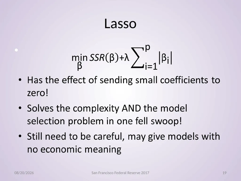
slide19. Lasso 11/3/2017 San Francisco Federal Reserve 2017 19<br>
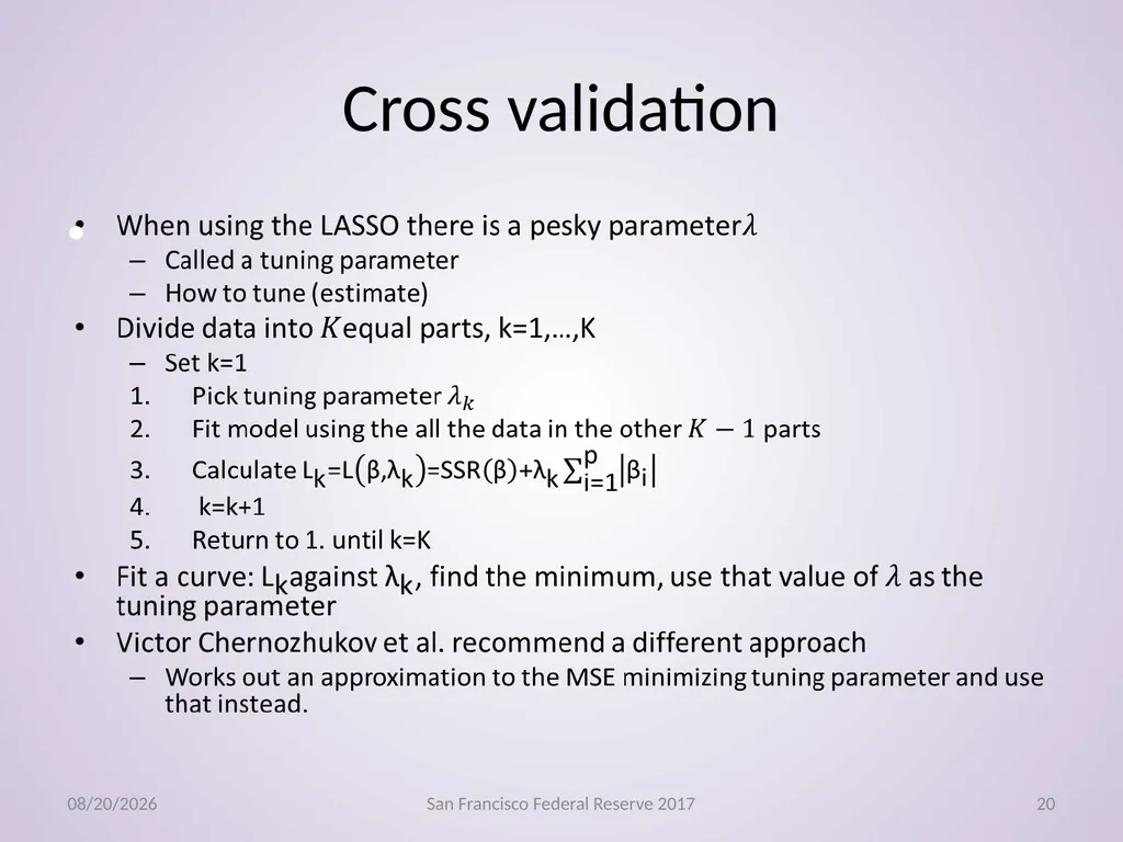
slide20. Cross validation 11/3/2017 San Francisco Federal Reserve 2017 20<br>
slide21. The test-train-cross validate paradigm is a key contribution of ML to econometrics 11/3/2017 San Francisco Federal Reserve 2017 21<br>
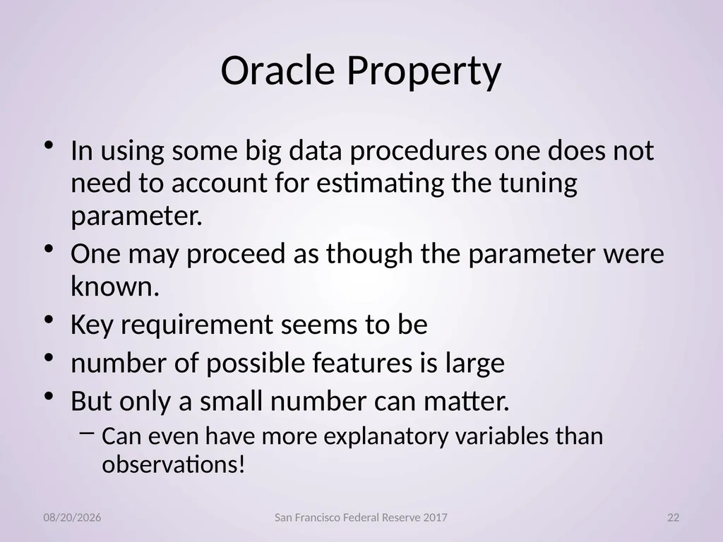
slide22. Oracle Property In using some big data procedures one does not need to account for estimating the tuning parameter.
One may proceed as though the parameter were known.
Key requirement seems to be
number of possible features is large
But only a small number can matter.
Can even have more explanatory variables than observations! 11/3/2017 San Francisco Federal Reserve 2017 22<br>
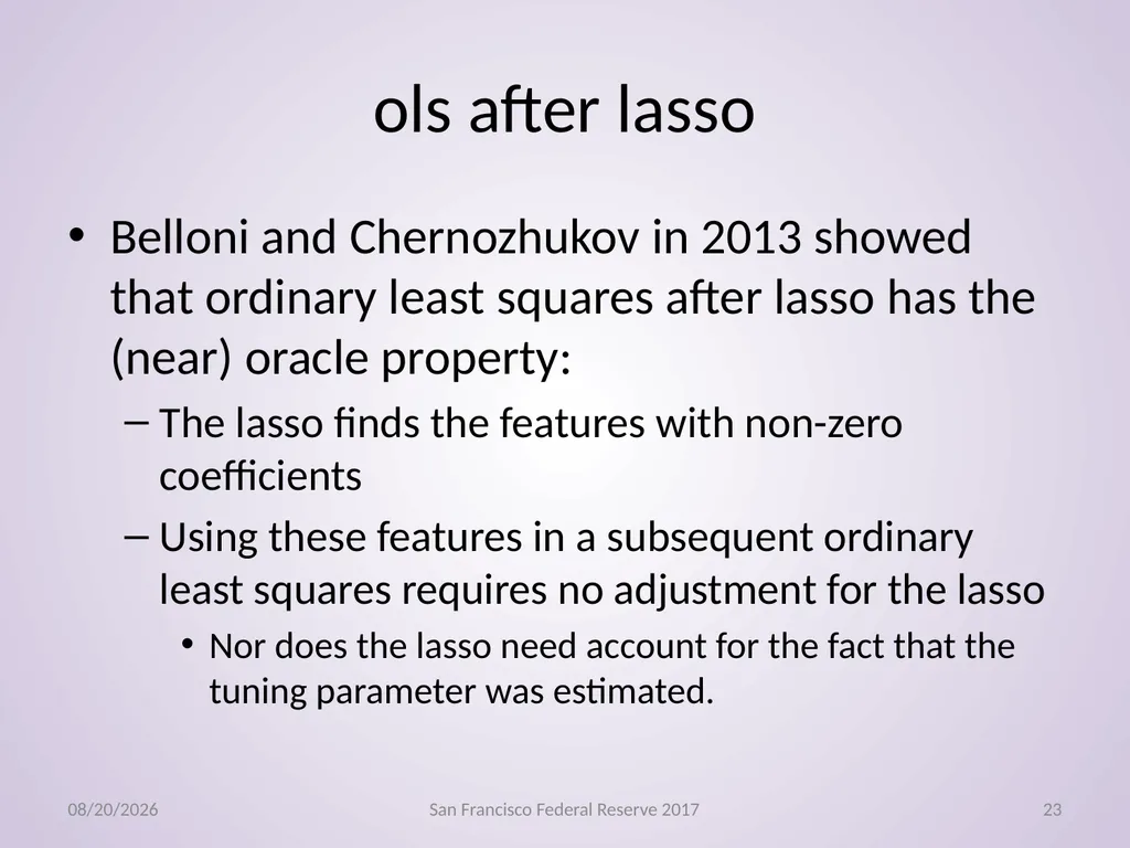
slide23. ols after lasso Belloni and Chernozhukov in 2013 showed that ordinary least squares after lasso has the (near) oracle property:
The lasso finds the features with non-zero coefficients
Using these features in a subsequent ordinary least squares requires no adjustment for the lasso
Nor does the lasso need account for the fact that the tuning parameter was estimated. 11/3/2017 San Francisco Federal Reserve 2017 23<br>
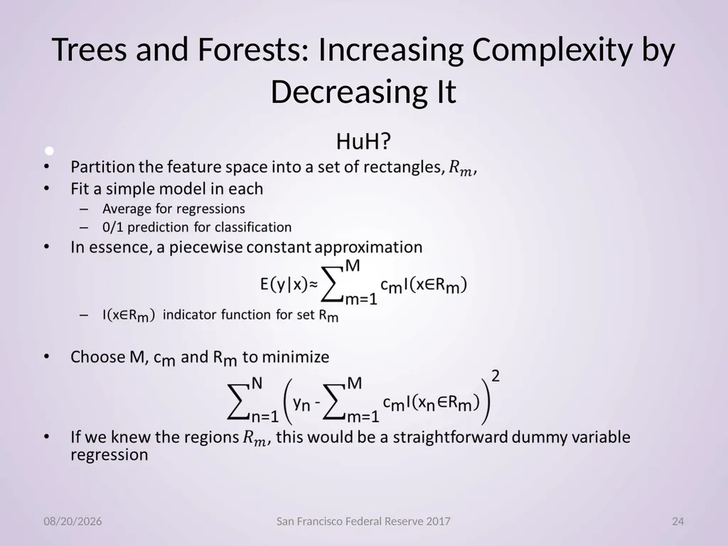
slide24. Trees and Forests: Increasing Complexity by Decreasing It 11/3/2017 San Francisco Federal Reserve 2017 24<br>
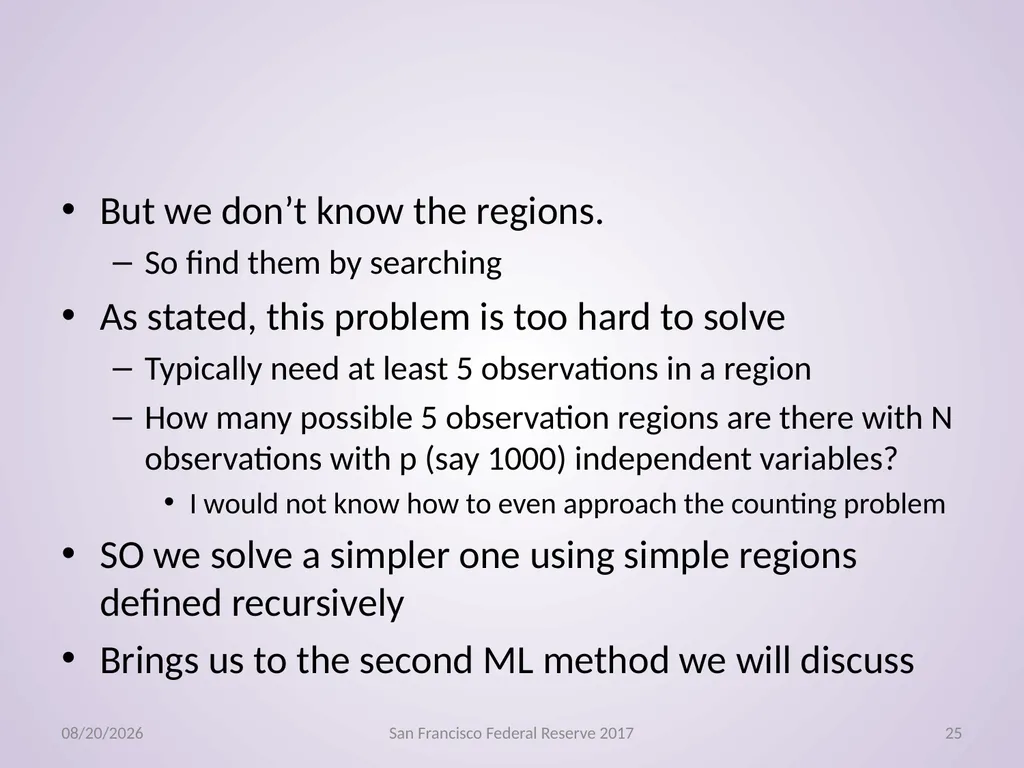
slide25. But we don’t know the regions.
So find them by searching
As stated, this problem is too hard to solve
Typically need at least 5 observations in a region
How many possible 5 observation regions are there with N observations with p (say 1000) independent variables?
I would not know how to even approach the counting problem
SO we solve a simpler one using simple regions defined recursively
Brings us to the second ML method we will discuss 11/3/2017 San Francisco Federal Reserve 2017 25<br>
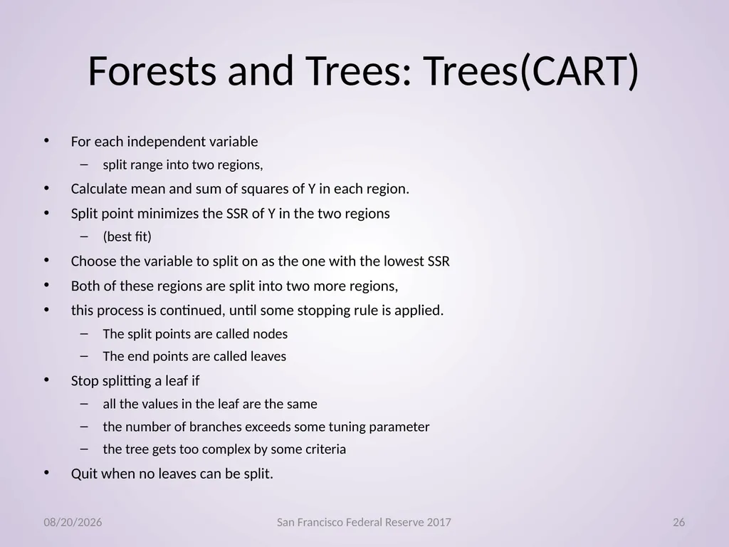
slide26. Forests and Trees: Trees(CART) For each independent variable
split range into two regions,
Calculate mean and sum of squares of Y in each region.
Split point minimizes the SSR of Y in the two regions
(best fit)
Choose the variable to split on as the one with the lowest SSR
Both of these regions are split into two more regions,
this process is continued, until some stopping rule is applied.
The split points are called nodes
The end points are called leaves
Stop splitting a leaf if
all the values in the leaf are the same
the number of branches exceeds some tuning parameter
the tree gets too complex by some criteria
Quit when no leaves can be split. 11/3/2017 San Francisco Federal Reserve 2017 26<br>
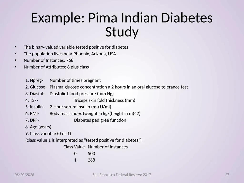
slide27. Example: Pima Indian Diabetes Study The binary-valued variable tested positive for diabetes
The population lives near Phoenix, Arizona, USA.
Number of Instances: 768
Number of Attributes: 8 plus class
1. Npreg- Number of times pregnant
2. Glucose- Plasma glucose concentration a 2 hours in an oral glucose tolerance test
3. Diastol- Diastolic blood pressure (mm Hg)
4. TSF- Triceps skin fold thickness (mm)
5. Insulin- 2-Hour serum insulin (mu U/ml)
6. BMI- Body mass index (weight in kg/(height in m)^2)
7. DPF- Diabetes pedigree function
8. Age (years)
9. Class variable (0 or 1)
(class value 1 is interpreted as "tested positive for diabetes")
Class Value Number of instances
0 500
1 268 11/3/2017 San Francisco Federal Reserve 2017 27<br>
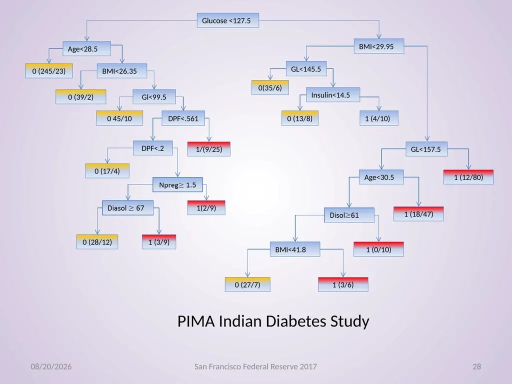
slide28. 11/3/2017 San Francisco Federal Reserve 2017 28 Glucose <127.5 Age<28.5 0 (245/23) BMI<26.35 0 (39/2) Gl<99.5 0 45/10 DPF<.561 1/(9/25) 0 (17/4) DPF<.2 1(2/9) 0 (28/12) 1 (3/9) BMI<29.95 GL<145.5 GL<157.5 Insulin<14.5 0(35/6) 1 (4/10) 0 (13/8) 1 (12/80) Age<30.5 1 (18/47) 1 (0/10) BMI<41.8 1 (3/6) 0 (27/7) PIMA Indian Diabetes Study<br>
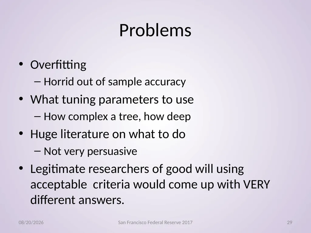
slide29. Problems Overfitting
Horrid out of sample accuracy
What tuning parameters to use
How complex a tree, how deep
Huge literature on what to do
Not very persuasive
Legitimate researchers of good will using acceptable criteria would come up with VERY different answers. 11/3/2017 San Francisco Federal Reserve 2017 29<br>
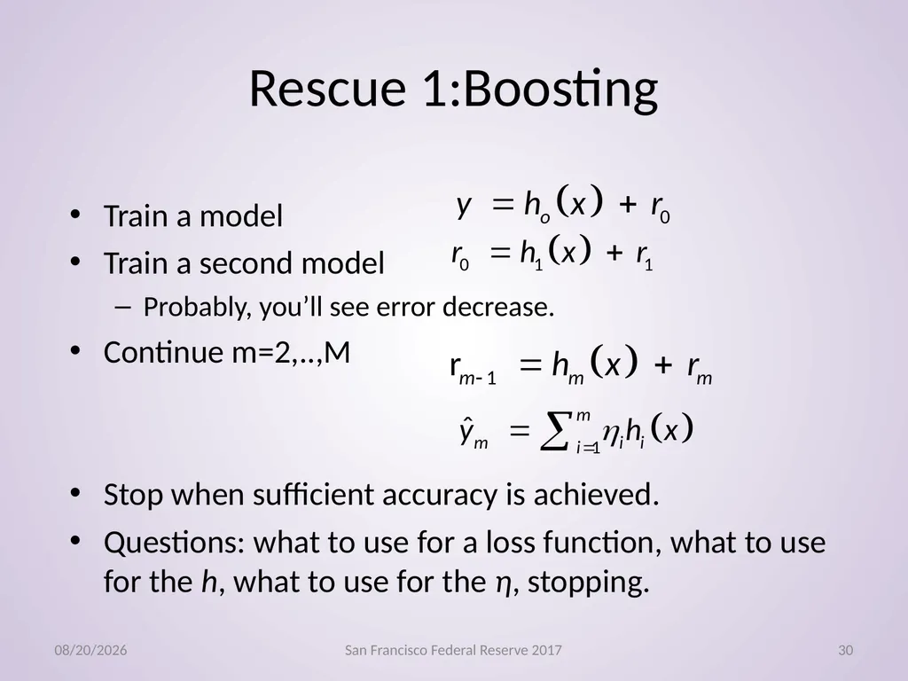
slide30. Rescue 1:Boosting Train a model
Train a second model
Probably, you’ll see error decrease.
Continue m=2,..,M
Stop when sufficient accuracy is achieved.
Questions: what to use for a loss function, what to use for the h, what to use for the η, stopping. 11/3/2017 San Francisco Federal Reserve 2017 30<br>
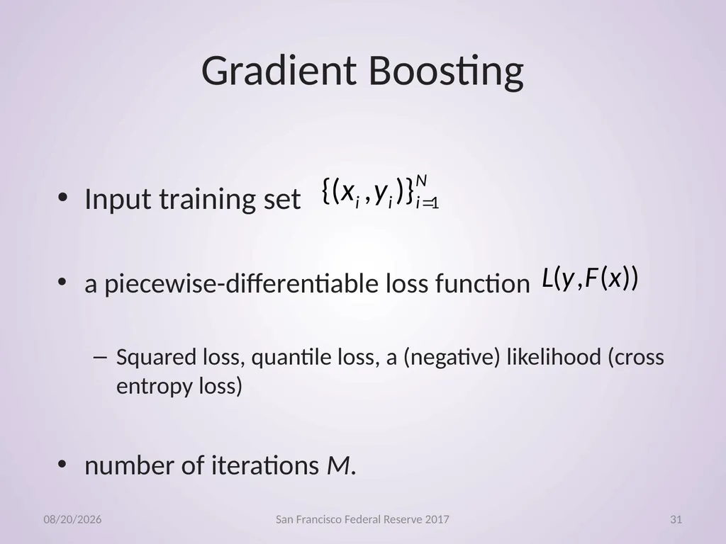
slide31. Input training set
a piecewise-differentiable loss function
Squared loss, quantile loss, a (negative) likelihood (cross entropy loss)
number of iterations M. Gradient Boosting 11/3/2017 San Francisco Federal Reserve 2017 31<br>
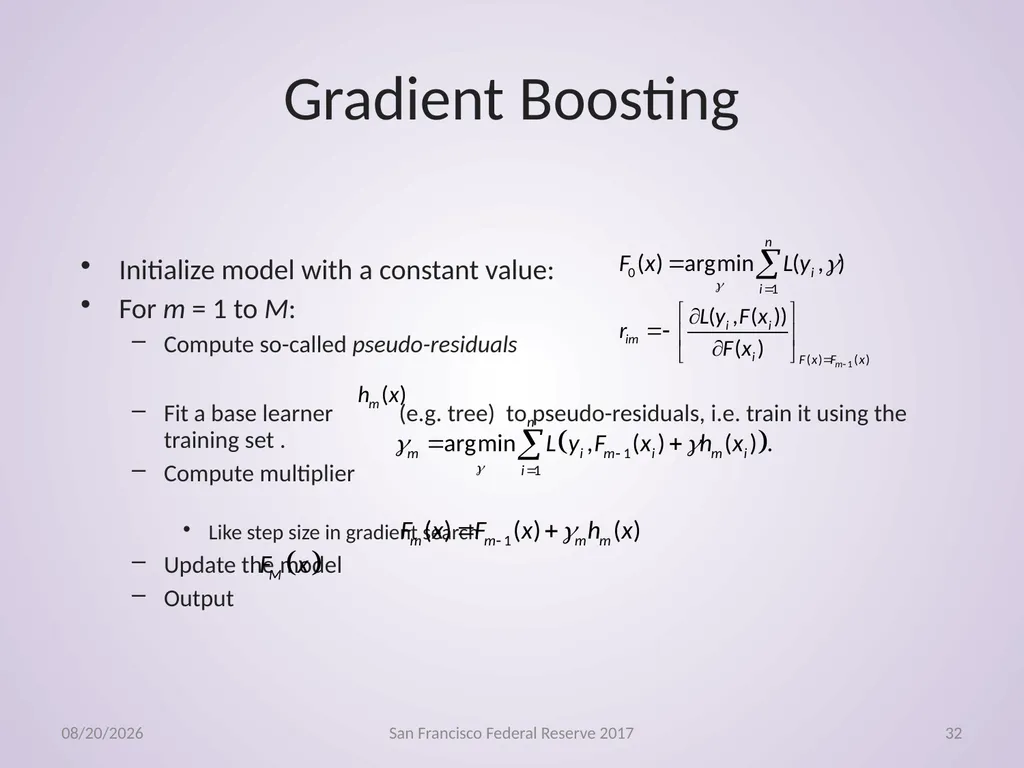
slide32. Initialize model with a constant value:
For m = 1 to M:
Compute so-called pseudo-residuals
Fit a base learner (e.g. tree) to pseudo-residuals, i.e. train it using the training set .
Compute multiplier
Like step size in gradient search
Update the model
Output Gradient Boosting 11/3/2017 San Francisco Federal Reserve 2017 32<br>
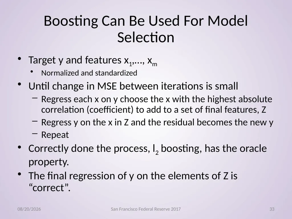
slide33. Boosting Can Be Used For Model Selection Target y and features x1,…, xm
Normalized and standardized
Until change in MSE between iterations is small
Regress each x on y choose the x with the highest absolute correlation (coefficient) to add to a set of final features, Z
Regress y on the x in Z and the residual becomes the new y
Repeat
Correctly done the process, l2 boosting, has the oracle property.
The final regression of y on the elements of Z is “correct”. 11/3/2017 San Francisco Federal Reserve 2017 33<br>
slide34. Boosting Rarely Overfits Repeat!!
Boosting Rarely Overfits 11/3/2017 San Francisco Federal Reserve 2017 34<br>
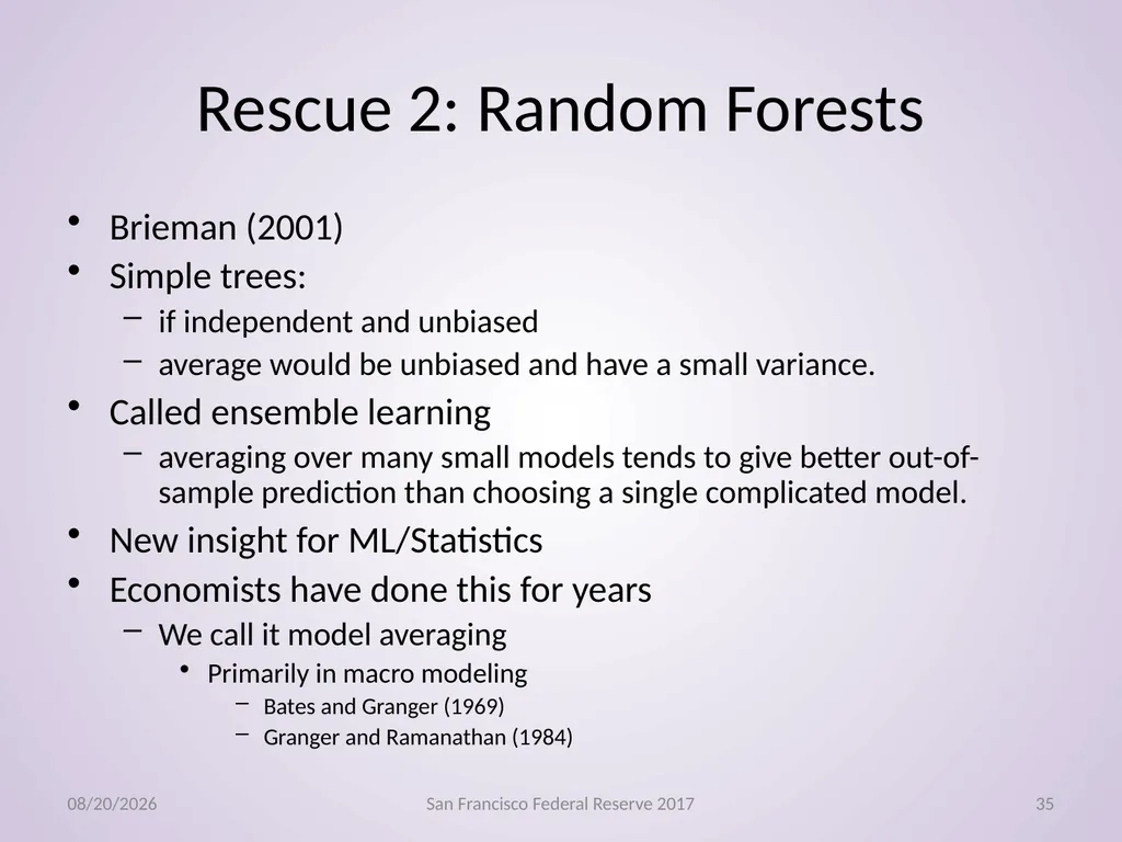
slide35. Rescue 2: Random Forests Brieman (2001)
Simple trees:
if independent and unbiased
average would be unbiased and have a small variance.
Called ensemble learning
averaging over many small models tends to give better out-of-sample prediction than choosing a single complicated model.
New insight for ML/Statistics
Economists have done this for years
We call it model averaging
Primarily in macro modeling
Bates and Granger (1969)
Granger and Ramanathan (1984) 11/3/2017 San Francisco Federal Reserve 2017 35<br>
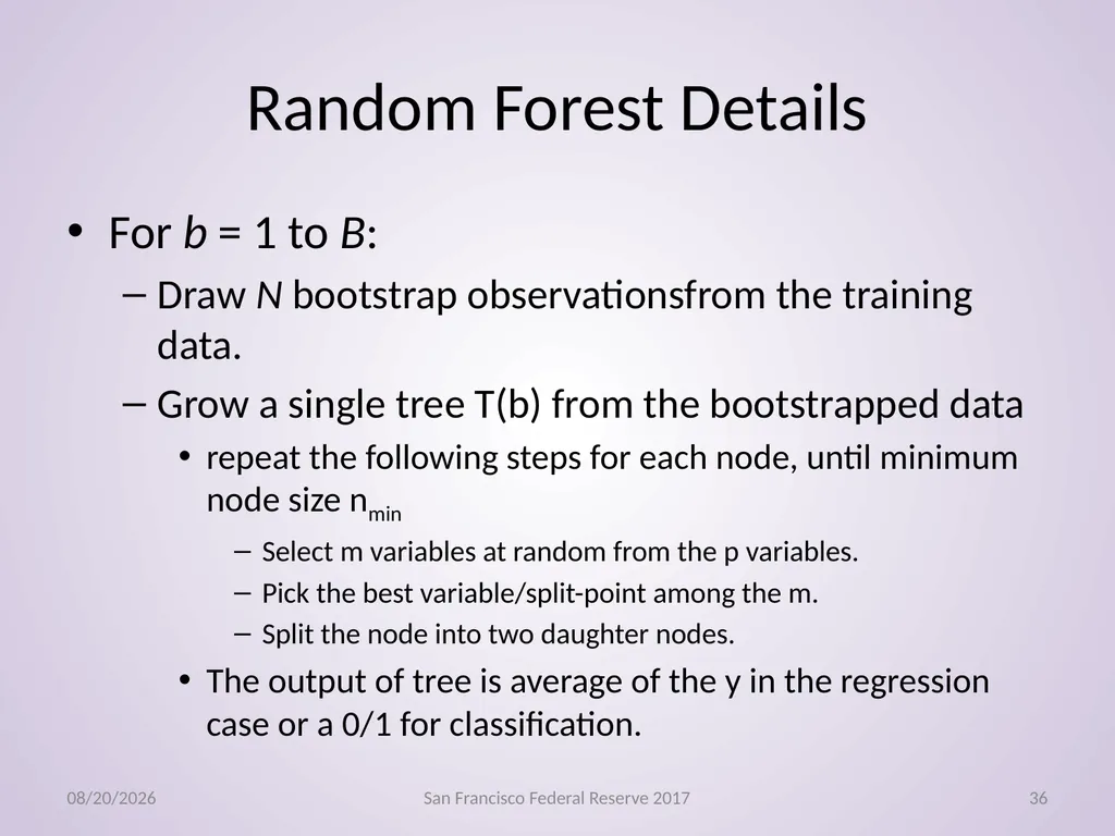
slide36. Random Forest Details For b = 1 to B:
Draw N bootstrap observationsfrom the training data.
Grow a single tree T(b) from the bootstrapped data
repeat the following steps for each node, until minimum node size nmin
Select m variables at random from the p variables.
Pick the best variable/split-point among the m.
Split the node into two daughter nodes.
The output of tree is average of the y in the regression case or a 0/1 for classification. 11/3/2017 San Francisco Federal Reserve 2017 36<br>
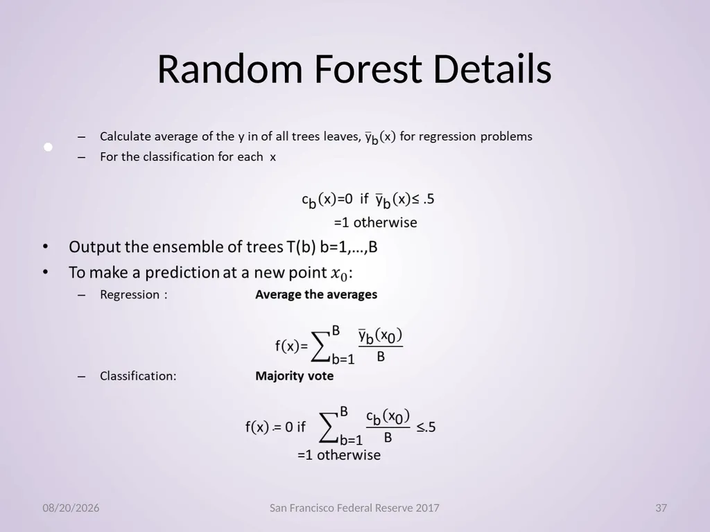
slide37. Random Forest Details 11/3/2017 San Francisco Federal Reserve 2017 37<br>
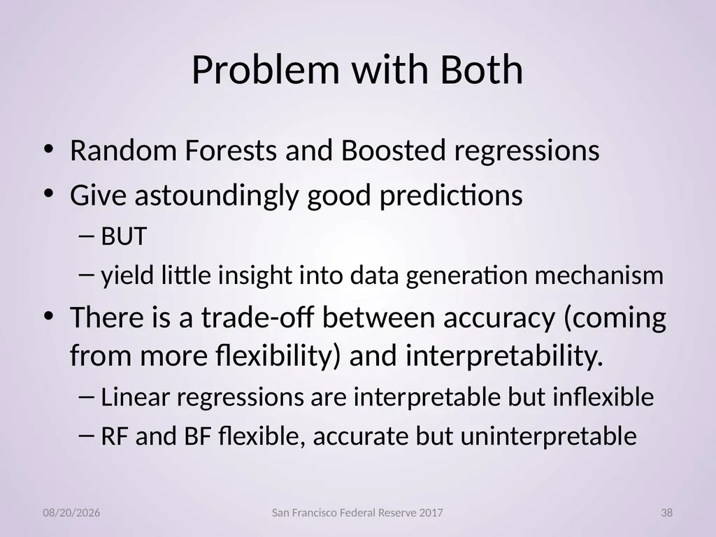
slide38. Problem with Both Random Forests and Boosted regressions
Give astoundingly good predictions
BUT
yield little insight into data generation mechanism
There is a trade-off between accuracy (coming from more flexibility) and interpretability.
Linear regressions are interpretable but inflexible
RF and BF flexible, accurate but uninterpretable 11/3/2017 San Francisco Federal Reserve 2017 38<br>
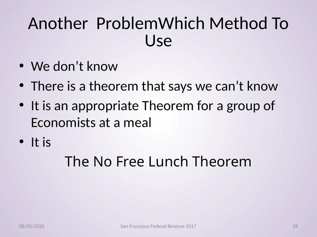
slide39. Another ProblemWhich Method To Use We don’t know
There is a theorem that says we can’t know
It is an appropriate Theorem for a group of Economists at a meal
It is
The No Free Lunch Theorem 11/3/2017 San Francisco Federal Reserve 2017 39<br>
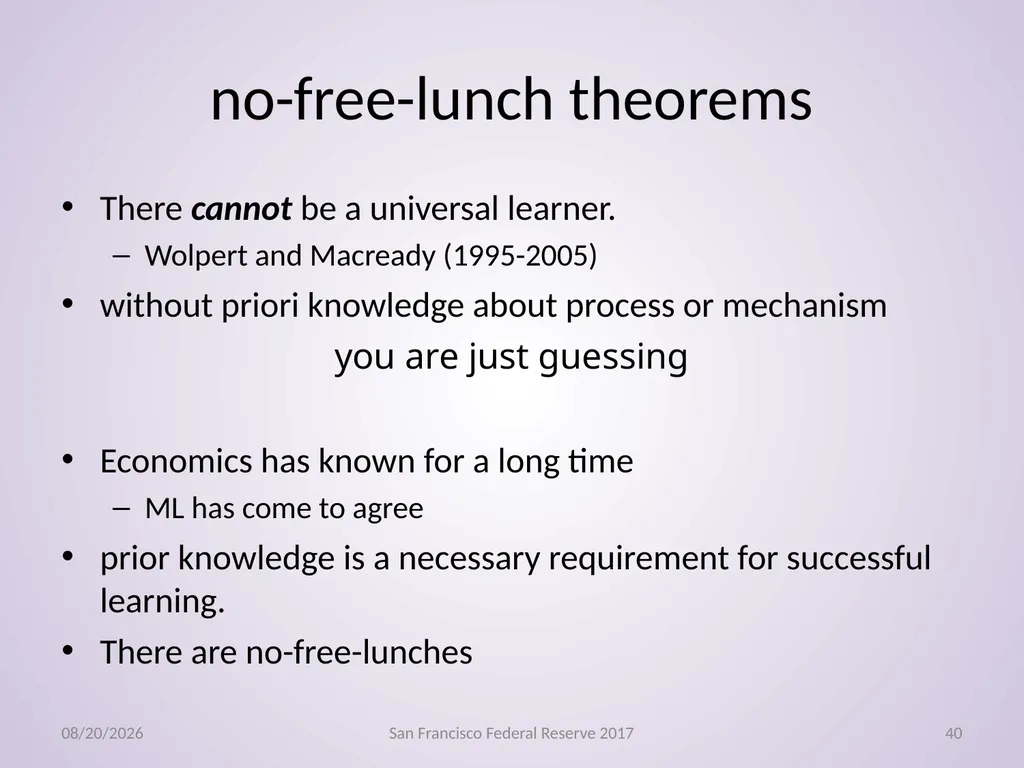
slide40. no-free-lunch theorems There cannot be a universal learner.
Wolpert and Macready (1995-2005)
without priori knowledge about process or mechanism
you are just guessing
Economics has known for a long time
ML has come to agree
prior knowledge is a necessary requirement for successful learning.
There are no-free-lunches 11/3/2017 San Francisco Federal Reserve 2017 40<br>
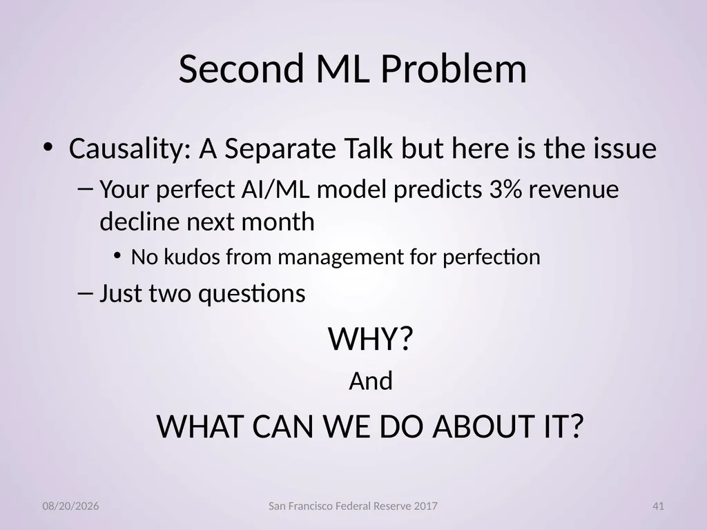
slide41. Second ML Problem Causality: A Separate Talk but here is the issue
Your perfect AI/ML model predicts 3% revenue decline next month
No kudos from management for perfection
Just two questions
WHY?
And
WHAT CAN WE DO ABOUT IT? 11/3/2017 San Francisco Federal Reserve 2017 41<br>
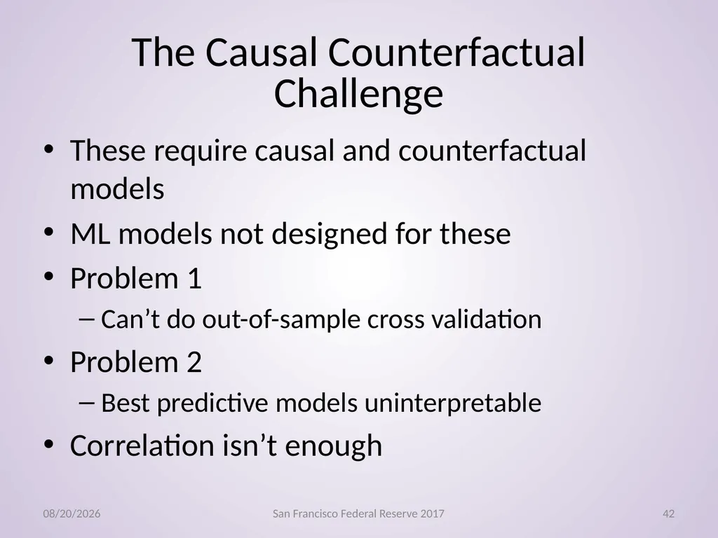
slide42. The Causal Counterfactual Challenge These require causal and counterfactual models
ML models not designed for these
Problem 1
Can’t do out-of-sample cross validation
Problem 2
Best predictive models uninterpretable
Correlation isn’t enough 11/3/2017 San Francisco Federal Reserve 2017 42<br>
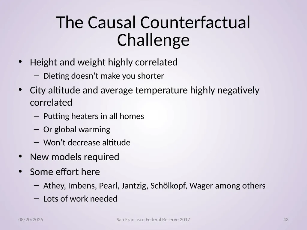
slide43. The Causal Counterfactual Challenge Height and weight highly correlated
Dieting doesn’t make you shorter
City altitude and average temperature highly negatively correlated
Putting heaters in all homes
Or global warming
Won’t decrease altitude
New models required
Some effort here
Athey, Imbens, Pearl, Jantzig, Schölkopf, Wager among others
Lots of work needed 11/3/2017 San Francisco Federal Reserve 2017 43<br>
slide44. The Causal Counterfactual Challenge Economists have contributed lots of work on the identification side starting with Reirosol, Marschak and Hurwicz.
More recently Chesher, Chernozhukov, Matzkin, Newey 11/3/2017 San Francisco Federal Reserve 2017 44<br>
slide45. The End 11/3/2017 San Francisco Federal Reserve 2017 45<br>
slide46. References of Particular Interest Breiman, L.,(2001), Statistical Modeling: The Two Cultures (with comments and a rejoinder by the author), Statistical Science, Volume 16, Issue 3 (2001), 199-231. https://projecteuclid.org/euclid.ss/1009213726
Efron, B., and Trevor Hastie (2016). Computer Age Statistical Inference: Algorithms, Evidence, and Data Science (Institute of Mathematical Statistics Monographs). Cambridge: Cambridge University Press. https://web.stanford.edu/~hastie/CASI/
Donoho, David (2015) 50 years of Data Science. Tukey Centennial Workshop, Princeton NJ Sept 18 2015. http://pages.cs.wisc.edu/~anhai/courses/784-fall15/50YearsDataScience.pdf
James, Gareth, Daniela Witten, Trevor Hastie and Robert Tibshirani (2015) An Introduction to Statistical Learning, with Applications in R, Springer.
http://www-bcf.usc.edu/~gareth/ISL/ISLR%20Sixth%20Printing.pdf
Harry J. Paarsch and Konstantin Golyaev (2016) A Gentle Introduction to Effective Computing in Quantitative Research: What Every Research Assistant Should Know, MIT Press.
Peters, Jonas, Dominik Janzing, and Bernhard Schölkopf(2017) Elements of Causal Inference:Foundations and Learning Algorithms, MIT Press
John W Tukey (1962) The future of data analysis. The Annals of Mathematical Statistics, 1–67. https://projecteuclid.org/download/pdf_1/euclid.aoms/1177704711 11/3/2017 San Francisco Federal Reserve 2017 46<br>
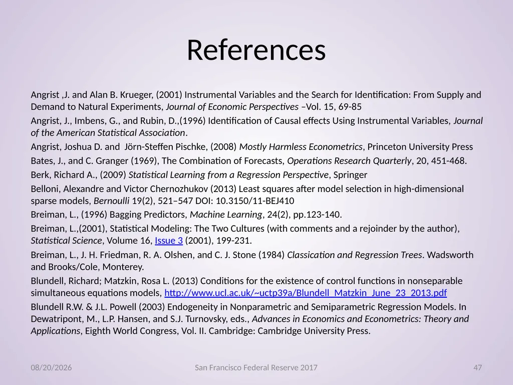
slide47. References Angrist ,J. and Alan B. Krueger, (2001) Instrumental Variables and the Search for Identification: From Supply and Demand to Natural Experiments, Journal of Economic Perspectives –Vol. 15, 69-85
Angrist, J., Imbens, G., and Rubin, D.,(1996) Identification of Causal effects Using Instrumental Variables, Journal of the American Statistical Association.
Angrist, Joshua D. and Jörn-Steffen Pischke, (2008) Mostly Harmless Econometrics, Princeton University Press
Bates, J., and C. Granger (1969), The Combination of Forecasts, Operations Research Quarterly, 20, 451-468.
Berk, Richard A., (2009) Statistical Learning from a Regression Perspective, Springer
Belloni, Alexandre and Victor Chernozhukov (2013) Least squares after model selection in high-dimensional sparse models, Bernoulli 19(2), 521–547 DOI: 10.3150/11-BEJ410
Breiman, L., (1996) Bagging Predictors, Machine Learning, 24(2), pp.123-140.
Breiman, L.,(2001), Statistical Modeling: The Two Cultures (with comments and a rejoinder by the author), Statistical Science, Volume 16, Issue 3 (2001), 199-231.
Breiman, L., J. H. Friedman, R. A. Olshen, and C. J. Stone (1984) Classication and Regression Trees. Wadsworth and Brooks/Cole, Monterey.
Blundell, Richard; Matzkin, Rosa L. (2013) Conditions for the existence of control functions in nonseparable simultaneous equations models, http://www.ucl.ac.uk/~uctp39a/Blundell_Matzkin_June_23_2013.pdf
Blundell R.W. & J.L. Powell (2003) Endogeneity in Nonparametric and Semiparametric Regression Models. In Dewatripont, M., L.P. Hansen, and S.J. Turnovsky, eds., Advances in Economics and Econometrics: Theory and Applications, Eighth World Congress, Vol. II. Cambridge: Cambridge University Press. 11/3/2017 San Francisco Federal Reserve 2017 47<br>
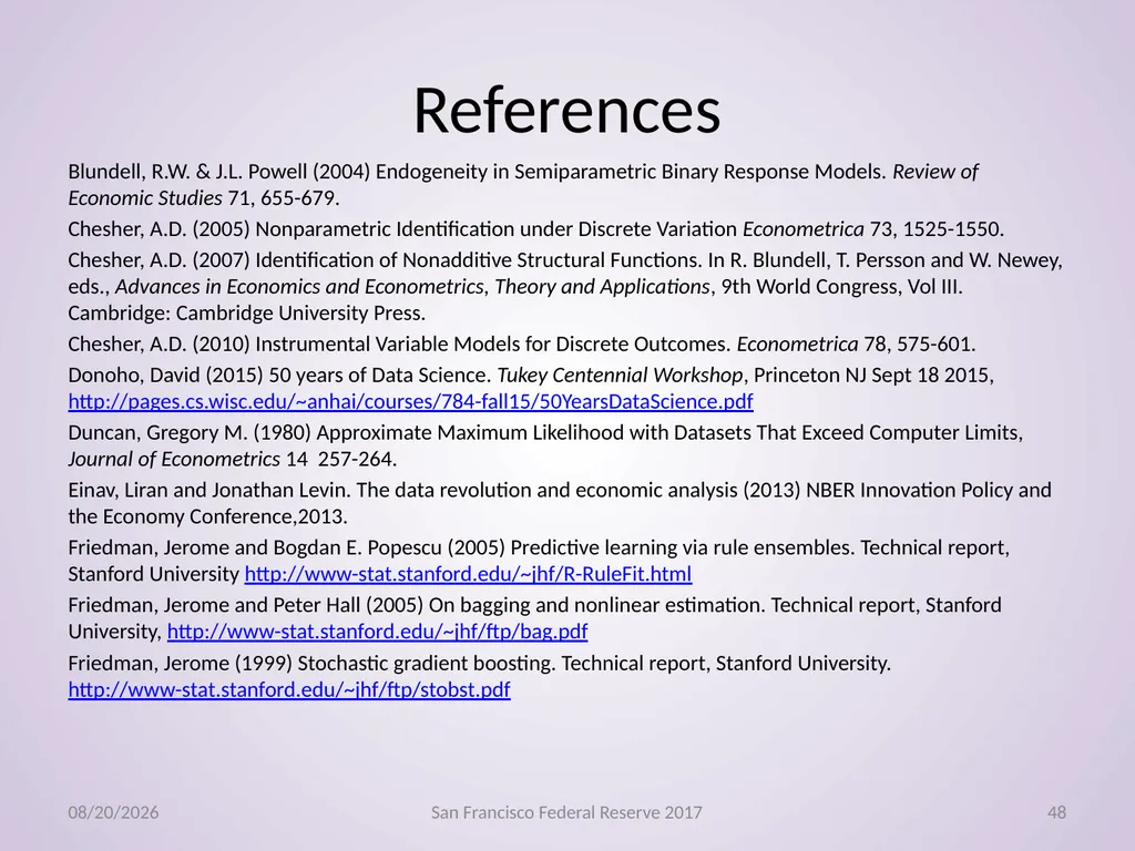
slide48. References Blundell, R.W. & J.L. Powell (2004) Endogeneity in Semiparametric Binary Response Models. Review of Economic Studies 71, 655-679.
Chesher, A.D. (2005) Nonparametric Identification under Discrete Variation Econometrica 73, 1525-1550.
Chesher, A.D. (2007) Identification of Nonadditive Structural Functions. In R. Blundell, T. Persson and W. Newey, eds., Advances in Economics and Econometrics, Theory and Applications, 9th World Congress, Vol III. Cambridge: Cambridge University Press.
Chesher, A.D. (2010) Instrumental Variable Models for Discrete Outcomes. Econometrica 78, 575-601.
Donoho, David (2015) 50 years of Data Science. Tukey Centennial Workshop, Princeton NJ Sept 18 2015, http://pages.cs.wisc.edu/~anhai/courses/784-fall15/50YearsDataScience.pdf
Duncan, Gregory M. (1980) Approximate Maximum Likelihood with Datasets That Exceed Computer Limits, Journal of Econometrics 14 257-264.
Einav, Liran and Jonathan Levin. The data revolution and economic analysis (2013) NBER Innovation Policy and the Economy Conference,2013.
Friedman, Jerome and Bogdan E. Popescu (2005) Predictive learning via rule ensembles. Technical report, Stanford University http://www-stat.stanford.edu/~jhf/R-RuleFit.html
Friedman, Jerome and Peter Hall (2005) On bagging and nonlinear estimation. Technical report, Stanford University, http://www-stat.stanford.edu/~jhf/ftp/bag.pdf
Friedman, Jerome (1999) Stochastic gradient boosting. Technical report, Stanford University. http://www-stat.stanford.edu/~jhf/ftp/stobst.pdf 11/3/2017 San Francisco Federal Reserve 2017 48<br>
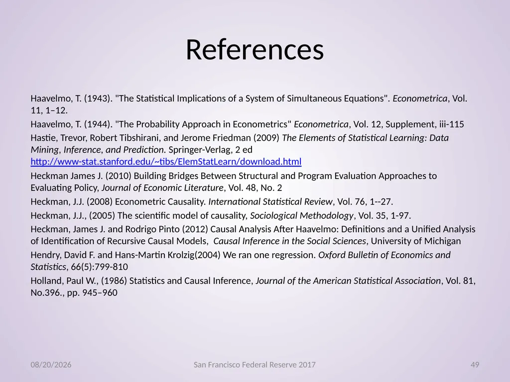
slide49. References Haavelmo, T. (1943). "The Statistical Implications of a System of Simultaneous Equations". Econometrica, Vol. 11, 1–12.
Haavelmo, T. (1944). "The Probability Approach in Econometrics" Econometrica, Vol. 12, Supplement, iii-115
Hastie, Trevor, Robert Tibshirani, and Jerome Friedman (2009) The Elements of Statistical Learning: Data Mining, Inference, and Prediction. Springer-Verlag, 2 ed http://www-stat.stanford.edu/~tibs/ElemStatLearn/download.html
Heckman James J. (2010) Building Bridges Between Structural and Program Evaluation Approaches to Evaluating Policy, Journal of Economic Literature, Vol. 48, No. 2
Heckman, J.J. (2008) Econometric Causality. International Statistical Review, Vol. 76, 1--27.
Heckman, J.J., (2005) The scientific model of causality, Sociological Methodology, Vol. 35, 1-97.
Heckman, James J. and Rodrigo Pinto (2012) Causal Analysis After Haavelmo: Definitions and a Unified Analysis of Identification of Recursive Causal Models, Causal Inference in the Social Sciences, University of Michigan
Hendry, David F. and Hans-Martin Krolzig(2004) We ran one regression. Oxford Bulletin of Economics and Statistics, 66(5):799-810
Holland, Paul W., (1986) Statistics and Causal Inference, Journal of the American Statistical Association, Vol. 81, No.396., pp. 945–960 11/3/2017 San Francisco Federal Reserve 2017 49<br>
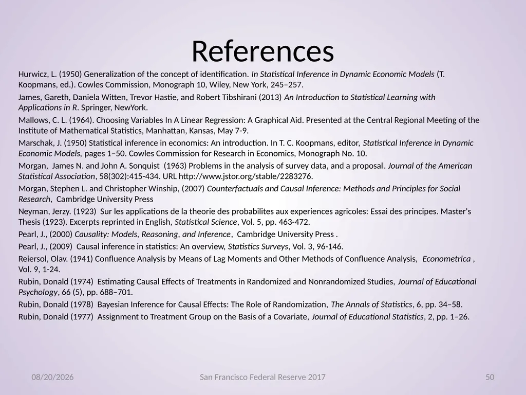
slide50. References Hurwicz, L. (1950) Generalization of the concept of identification. In Statistical Inference in Dynamic Economic Models (T. Koopmans, ed.). Cowles Commission, Monograph 10, Wiley, New York, 245–257.
James, Gareth, Daniela Witten, Trevor Hastie, and Robert Tibshirani (2013) An Introduction to Statistical Learning with Applications in R. Springer, NewYork.
Mallows, C. L. (1964). Choosing Variables In A Linear Regression: A Graphical Aid. Presented at the Central Regional Meeting of the Institute of Mathematical Statistics, Manhattan, Kansas, May 7-9.
Marschak, J. (1950) Statistical inference in economics: An introduction. In T. C. Koopmans, editor, Statistical Inference in Dynamic Economic Models, pages 1–50. Cowles Commission for Research in Economics, Monograph No. 10.
Morgan, James N. and John A. Sonquist (1963) Problems in the analysis of survey data, and a proposal. Journal of the American Statistical Association, 58(302):415-434. URL http://www.jstor.org/stable/2283276.
Morgan, Stephen L. and Christopher Winship, (2007) Counterfactuals and Causal Inference: Methods and Principles for Social Research, Cambridge University Press
Neyman, Jerzy. (1923) Sur les applications de la theorie des probabilites aux experiences agricoles: Essai des principes. Master's Thesis (1923). Excerpts reprinted in English, Statistical Science, Vol. 5, pp. 463-472.
Pearl, J., (2000) Causality: Models, Reasoning, and Inference, Cambridge University Press .
Pearl, J., (2009) Causal inference in statistics: An overview, Statistics Surveys, Vol. 3, 96-146.
Reiersol, Olav. (1941) Confluence Analysis by Means of Lag Moments and Other Methods of Confluence Analysis, Econometrica , Vol. 9, 1-24.
Rubin, Donald (1974) Estimating Causal Effects of Treatments in Randomized and Nonrandomized Studies, Journal of Educational Psychology, 66 (5), pp. 688–701.
Rubin, Donald (1978) Bayesian Inference for Causal Effects: The Role of Randomization, The Annals of Statistics, 6, pp. 34–58.
Rubin, Donald (1977) Assignment to Treatment Group on the Basis of a Covariate, Journal of Educational Statistics, 2, pp. 1–26. 11/3/2017 San Francisco Federal Reserve 2017 50<br>
slide51. References Shpitser, I. and Pearl, J.,(2006) Identification of Conditional Interventional Distributions. In R. Dechter and T.S. Richardson (Eds.), Proceedings of the Twenty-Second Conference on Uncertainty in Artificial Intelligence, Corvallis, OR: AUAI Press, 437-444.
Wu, Xindong and Vipin Kumar, editors. The Top Ten Algorithms in Data Mining. CRC Press, 2009. URL http://www.cs.uvm.edu/~icdm/algorithms/index.shtml 11/3/2017 San Francisco Federal Reserve 2017 51<br>
Amazon.com
University of Washington and All that stuff<br>
slide2. Introduction Vast data available today
hundreds of billions of observations and millions of features
A 100,000,000,000 x 1,500,000 dimensional tables/matrices common
Allows analyses unthinkable 15 years ago
Presents challenges to econometricians, computer scientists and statisticians
How to get that matrix into a computer
Can you get that matrix into a computer
If so how do you interpret 1.5 million independent variables
Can you interpret 1.5 million independent variables 11/3/2017 San Francisco Federal Reserve 2017 2<br>
slide3. Approaches Very different approaches, and languages
Econometricians (and other social scientists)
What is the probability model for the data
Interested primarily in gaining insight into behavioral processes
Sometimes prediction
Statisticians
How to make inference for data from general probability models
Computer scientists
How to compute 11/3/2017 San Francisco Federal Reserve 2017 3<br>
slide4. Culture Wars Brieman(2000)
ML
How does the model predict out-of-sample
Proofs of properties more-or-less useless
Let data reveal structure
Statistics
What is the underlying probability model
How to infer structure
How to predict using structure
Economics
Much like Stat
Though economist and nearly as famous Economist Milton Friedman was clearly amenable to the ML camp
I would add Sims as well. 11/3/2017 San Francisco Federal Reserve 2017 4<br>
slide5. Overview Introduction to the intersection for economists.
Computer Science will tell you that they invented “big data” methods
Actually, a lot comes from economics
This will be a theme.
Much of the new stuff is quite old.
Impossible to do in its day
Made Possible by Advances in CS and Statistics 11/3/2017 San Francisco Federal Reserve 2017 5<br>
slide6. Sidebar Machine Learning is a chair with three legs
Statistics
Computer Science
Domain knowledge(Bio-Science, Econometrics)
Each group seems to give at best lip service to the others
Biotech has shown the way
Social Sciences and Statistics Lag 11/3/2017 San Francisco Federal Reserve 2017 6<br>
slide7. Econometrics in Machine Learning Causality and identification
Economics 1950
Leonid Hurwicz (Economics 2007, Nobel Prize winner)(U Minnesota)
Computer Science 1998
Judea Pearl (UCLA)
Tree methods
Economics 1963
James N. Morgan (U of Michigan)
Statistics 1984
Leo Brieman (Berkeley)
Map Reduce
Economics 1980
Me (Northwestern)
Computer Science 2004
Jeffrey Dean and Sanjay Ghemawat (Google) 11/3/2017 San Francisco Federal Reserve 2017 7<br>
slide8. Econometrics in Machine Learning Bagging/Ensemble Methods
Economics 1969
Bates and Granger (UCSD)
ML 1996
Brieman (almost of course)
Economists early contributors to neural net/deep learning literature (late 1980’s early 1990’s)
Hal White, Jeff Wooldridge, Ron Gallant, Max Stinchcombe
Quantile neural nets, learning derivatives, guarantees for convergence, distributions etc.
Needed for counterfactuals when out of sample validation make no conceptual sense 11/3/2017 San Francisco Federal Reserve 2017 8<br>
slide9. Much of machine learning
rediscovers old statistical and econometric methods
but making them blindingly fast and practicable
This is not damning with faint praise
Many of the tools used today have been enabled purely by computers
Bootstrap (1984)
resampling
SAS (1966, but really 1976)
Huge datasets
TSP (1966)
UI
Albeit command line
Principled Model Selection (Lasso, L2-boosting) 11/3/2017 San Francisco Federal Reserve 2017 9<br>
slide10. Outcome of machine learning is generally a data reduction
Regression coefficients
Summary statistics
A prediction
Machine learning allows more complex models than economists are used to
I will focus on regression-like tools 11/3/2017 San Francisco Federal Reserve 2017 10<br>
slide11. Regression Setup 11/3/2017 San Francisco Federal Reserve 2017 11<br>
slide12. ML Approach ML would use
GLMs
Neural Nets
Support Vector Machines
Boosting
Regularization methods
Ridge
Lasso
Elastic Net
Classification and regression trees (CART)
Random forests 11/3/2017 San Francisco Federal Reserve 2017 12<br>
slide13. I will concentrate on the last 4
In all 4 of these, the ML goal is getting good out-of-sample predictions
Good for their own sake
ML believes good-out-of-sample predictions imply
a implicit consistent estimate of the underlying data generation process 11/3/2017 San Francisco Federal Reserve 2017 13<br>
slide14. First ML Problem: Overfitting It is quite easy to obtain models that give nearly perfect in-sample predictions
But the model fails disastrously out of sample.
This is referred to as overfitting
ML has developed a number of incredibly useful methods for handling overfitting.
One such is 11/3/2017 San Francisco Federal Reserve 2017 14<br>
slide15. Out of Sample Validation Divide data into subsets for the purpose of estimation, testing and validation
Training data used to estimate
Estimated model predicts on the validation set and compared to actual.
Similarly for testing.
Economists have taught this for years
Few if any ever did it
Too little data
Another such is 11/3/2017 San Francisco Federal Reserve 2017 15<br>
slide16. Regularization 11/3/2017 San Francisco Federal Reserve 2017 16<br>
slide17. 11/3/2017 San Francisco Federal Reserve 2017 17<br>
slide18. Or 402,387,260,077,093,773,543,702,433,923,003,985,719,374,864,210,714,632,543,799,910,429,938,512,398,629,020,592,044,208,486,969,404,800,479,988,610,197,196,058,631,666,872,994,808,558,901,323,829,669,944,590,997,424,504,087,073,759,918,823,627,727,188,732,519,779,505,950,995,276,120,874,975,462,497,043,601,418,278,094,646,496,291,056,393,887,437,886,487,337,119,181,045,825,783,647,849,977,012,476,632,889,835,955,735,432,513,185,323,958,463,075,557,409,114,262,417,474,349,347,553,428,646,576,611,667,797,396,668,820,291,207,379,143,853,719,588,249,808,126,867,838,374,559,731,746,136,085,379,534,524,221,586,593,201,928,090,878,297,308,431,392,844,403,281,231,558,611,036,976,801,357,304,216,168,747,609,675,871,348,312,025,478,589,320,767,169,132,448,426,236,131,412,508,780,208,000,261,683,151,027,341,827,977,704,784,635,868,170,164,365,024,153,691,398,281,264,810,213,092,761,244,896,359,928,705,114,964,975,419,909,342,221,566,832,572,080,821,333,186,116,811,553,615,836,546,984,046,708,975,602,900,950,537,616,475,847,728,421,889,679,646,244,945,160,765,353,408,198,901,385,442,487,984,959,953,319,101,723,355,556,602,139,450,399,736,280,750,137,837,615,307,127,761,926,849,034,352,625,200,015,888,535,147,331,611,702,103,968,175,921,510,907,788,019,393,178,114,194,545,257,223,865,541,461,062,892,187,960,223,838,971,476,088,506,276,862,967,146,674,697,562,911,234,082,439,208,160,153,780,889,893,964,518,263,243,671,616,762,179,168,909,779,911,903,754,031,274,622,289,988,005,195,444,414,282,012,187,361,745,992,642,956,581,746,628,302,955,570,299,024,324,153,181,617,210,465,832,036,786,906,117,260,158,783,520,751,516,284,225,540,265,170,483,304,226,143,974,286,933,061,690,897,968,482,590,125,458,327,168,226,458,066,526,769,958,652,682,272,807,075,781,391,858,178,889,652,208,164,348,344,825,993,266,043,367,660,176,999,612,831,860,788,386,150,279,465,955,131,156,552,036,093,988,180,612,138,558,600,301,435,694,527,224,206,344,631,797,460,594,682,573,103,790,084,024,432,438,465,657,245,014,402,821,885,252,470,935,190,620,929,023,136,493,273,497,565,513,958,720,559,654,228,749,774,011,413,346,962,715,422,845,862,377,387,538,230,483,865,688,976,461,927,383,814,900,140,767,310,446,640,259,899,490,222,221,765,904,339,901,886,018,566,526,485,061,799,702,356,193,897,017,860,040,811,889,729,918,311,021,171,229,845,901,641,921,068,884,387,121,855,646,124,960,798,722,908,519,296,819,372,388,642,614,839,657,382,291,123,125,024,186,649,353,143,970,137,428,531,926,649,875,337,218,940,694,281,434,118,520,158,014,123,344,828,015,051,399,694,290,153,483,077,644,569,099,073,152,433,278,288,269,864,602,789,864,321,139,083,506,217,095,002,597,389,863,554,277,196,742,822,248,757,586,765,752,344,220,207,573,630,569,498,825,087,968,928,162,753,848,863,396,909,959,826,280,956,121,450,994,871,701,244,516,461,260,379,029,309,120,889,086,942,028,510,640,182,154,399,457,156,805,941,872,748,998,094,254,742,173,582,401,063,677,404,595,741,785,160,829,230,135,358,081,840,096,996,372,524,230,560,855,903,700,624,271,243,416,909,004,153,690,105,933,983,835,777,939,410,970,027,753,472,000,000,000,000,000,000,000,000,000,000,000,000,000,000,000,000,000,000,000,000,000,000,000,000,000,000,000,000,000,000,000,000,000,000,000,000,000,000,000,000,000,000,000,000,000,000,000,000,000,000,000,000,000,000,000,000,000,000,000,000,000,000,000,000,000,000,000,000,000,000,000,000,000,000,000,000,000,000,000,000,000
Whack off 7 of the zeros and divide by three to get the number of years to use Mallows method in a small ML problem 11/3/2017 San Francisco Federal Reserve 2017 18<br>
slide19. Lasso 11/3/2017 San Francisco Federal Reserve 2017 19<br>
slide20. Cross validation 11/3/2017 San Francisco Federal Reserve 2017 20<br>
slide21. The test-train-cross validate paradigm is a key contribution of ML to econometrics 11/3/2017 San Francisco Federal Reserve 2017 21<br>
slide22. Oracle Property In using some big data procedures one does not need to account for estimating the tuning parameter.
One may proceed as though the parameter were known.
Key requirement seems to be
number of possible features is large
But only a small number can matter.
Can even have more explanatory variables than observations! 11/3/2017 San Francisco Federal Reserve 2017 22<br>
slide23. ols after lasso Belloni and Chernozhukov in 2013 showed that ordinary least squares after lasso has the (near) oracle property:
The lasso finds the features with non-zero coefficients
Using these features in a subsequent ordinary least squares requires no adjustment for the lasso
Nor does the lasso need account for the fact that the tuning parameter was estimated. 11/3/2017 San Francisco Federal Reserve 2017 23<br>
slide24. Trees and Forests: Increasing Complexity by Decreasing It 11/3/2017 San Francisco Federal Reserve 2017 24<br>
slide25. But we don’t know the regions.
So find them by searching
As stated, this problem is too hard to solve
Typically need at least 5 observations in a region
How many possible 5 observation regions are there with N observations with p (say 1000) independent variables?
I would not know how to even approach the counting problem
SO we solve a simpler one using simple regions defined recursively
Brings us to the second ML method we will discuss 11/3/2017 San Francisco Federal Reserve 2017 25<br>
slide26. Forests and Trees: Trees(CART) For each independent variable
split range into two regions,
Calculate mean and sum of squares of Y in each region.
Split point minimizes the SSR of Y in the two regions
(best fit)
Choose the variable to split on as the one with the lowest SSR
Both of these regions are split into two more regions,
this process is continued, until some stopping rule is applied.
The split points are called nodes
The end points are called leaves
Stop splitting a leaf if
all the values in the leaf are the same
the number of branches exceeds some tuning parameter
the tree gets too complex by some criteria
Quit when no leaves can be split. 11/3/2017 San Francisco Federal Reserve 2017 26<br>
slide27. Example: Pima Indian Diabetes Study The binary-valued variable tested positive for diabetes
The population lives near Phoenix, Arizona, USA.
Number of Instances: 768
Number of Attributes: 8 plus class
1. Npreg- Number of times pregnant
2. Glucose- Plasma glucose concentration a 2 hours in an oral glucose tolerance test
3. Diastol- Diastolic blood pressure (mm Hg)
4. TSF- Triceps skin fold thickness (mm)
5. Insulin- 2-Hour serum insulin (mu U/ml)
6. BMI- Body mass index (weight in kg/(height in m)^2)
7. DPF- Diabetes pedigree function
8. Age (years)
9. Class variable (0 or 1)
(class value 1 is interpreted as "tested positive for diabetes")
Class Value Number of instances
0 500
1 268 11/3/2017 San Francisco Federal Reserve 2017 27<br>
slide28. 11/3/2017 San Francisco Federal Reserve 2017 28 Glucose <127.5 Age<28.5 0 (245/23) BMI<26.35 0 (39/2) Gl<99.5 0 45/10 DPF<.561 1/(9/25) 0 (17/4) DPF<.2 1(2/9) 0 (28/12) 1 (3/9) BMI<29.95 GL<145.5 GL<157.5 Insulin<14.5 0(35/6) 1 (4/10) 0 (13/8) 1 (12/80) Age<30.5 1 (18/47) 1 (0/10) BMI<41.8 1 (3/6) 0 (27/7) PIMA Indian Diabetes Study<br>
slide29. Problems Overfitting
Horrid out of sample accuracy
What tuning parameters to use
How complex a tree, how deep
Huge literature on what to do
Not very persuasive
Legitimate researchers of good will using acceptable criteria would come up with VERY different answers. 11/3/2017 San Francisco Federal Reserve 2017 29<br>
slide30. Rescue 1:Boosting Train a model
Train a second model
Probably, you’ll see error decrease.
Continue m=2,..,M
Stop when sufficient accuracy is achieved.
Questions: what to use for a loss function, what to use for the h, what to use for the η, stopping. 11/3/2017 San Francisco Federal Reserve 2017 30<br>
slide31. Input training set
a piecewise-differentiable loss function
Squared loss, quantile loss, a (negative) likelihood (cross entropy loss)
number of iterations M. Gradient Boosting 11/3/2017 San Francisco Federal Reserve 2017 31<br>
slide32. Initialize model with a constant value:
For m = 1 to M:
Compute so-called pseudo-residuals
Fit a base learner (e.g. tree) to pseudo-residuals, i.e. train it using the training set .
Compute multiplier
Like step size in gradient search
Update the model
Output Gradient Boosting 11/3/2017 San Francisco Federal Reserve 2017 32<br>
slide33. Boosting Can Be Used For Model Selection Target y and features x1,…, xm
Normalized and standardized
Until change in MSE between iterations is small
Regress each x on y choose the x with the highest absolute correlation (coefficient) to add to a set of final features, Z
Regress y on the x in Z and the residual becomes the new y
Repeat
Correctly done the process, l2 boosting, has the oracle property.
The final regression of y on the elements of Z is “correct”. 11/3/2017 San Francisco Federal Reserve 2017 33<br>
slide34. Boosting Rarely Overfits Repeat!!
Boosting Rarely Overfits 11/3/2017 San Francisco Federal Reserve 2017 34<br>
slide35. Rescue 2: Random Forests Brieman (2001)
Simple trees:
if independent and unbiased
average would be unbiased and have a small variance.
Called ensemble learning
averaging over many small models tends to give better out-of-sample prediction than choosing a single complicated model.
New insight for ML/Statistics
Economists have done this for years
We call it model averaging
Primarily in macro modeling
Bates and Granger (1969)
Granger and Ramanathan (1984) 11/3/2017 San Francisco Federal Reserve 2017 35<br>
slide36. Random Forest Details For b = 1 to B:
Draw N bootstrap observationsfrom the training data.
Grow a single tree T(b) from the bootstrapped data
repeat the following steps for each node, until minimum node size nmin
Select m variables at random from the p variables.
Pick the best variable/split-point among the m.
Split the node into two daughter nodes.
The output of tree is average of the y in the regression case or a 0/1 for classification. 11/3/2017 San Francisco Federal Reserve 2017 36<br>
slide37. Random Forest Details 11/3/2017 San Francisco Federal Reserve 2017 37<br>
slide38. Problem with Both Random Forests and Boosted regressions
Give astoundingly good predictions
BUT
yield little insight into data generation mechanism
There is a trade-off between accuracy (coming from more flexibility) and interpretability.
Linear regressions are interpretable but inflexible
RF and BF flexible, accurate but uninterpretable 11/3/2017 San Francisco Federal Reserve 2017 38<br>
slide39. Another ProblemWhich Method To Use We don’t know
There is a theorem that says we can’t know
It is an appropriate Theorem for a group of Economists at a meal
It is
The No Free Lunch Theorem 11/3/2017 San Francisco Federal Reserve 2017 39<br>
slide40. no-free-lunch theorems There cannot be a universal learner.
Wolpert and Macready (1995-2005)
without priori knowledge about process or mechanism
you are just guessing
Economics has known for a long time
ML has come to agree
prior knowledge is a necessary requirement for successful learning.
There are no-free-lunches 11/3/2017 San Francisco Federal Reserve 2017 40<br>
slide41. Second ML Problem Causality: A Separate Talk but here is the issue
Your perfect AI/ML model predicts 3% revenue decline next month
No kudos from management for perfection
Just two questions
WHY?
And
WHAT CAN WE DO ABOUT IT? 11/3/2017 San Francisco Federal Reserve 2017 41<br>
slide42. The Causal Counterfactual Challenge These require causal and counterfactual models
ML models not designed for these
Problem 1
Can’t do out-of-sample cross validation
Problem 2
Best predictive models uninterpretable
Correlation isn’t enough 11/3/2017 San Francisco Federal Reserve 2017 42<br>
slide43. The Causal Counterfactual Challenge Height and weight highly correlated
Dieting doesn’t make you shorter
City altitude and average temperature highly negatively correlated
Putting heaters in all homes
Or global warming
Won’t decrease altitude
New models required
Some effort here
Athey, Imbens, Pearl, Jantzig, Schölkopf, Wager among others
Lots of work needed 11/3/2017 San Francisco Federal Reserve 2017 43<br>
slide44. The Causal Counterfactual Challenge Economists have contributed lots of work on the identification side starting with Reirosol, Marschak and Hurwicz.
More recently Chesher, Chernozhukov, Matzkin, Newey 11/3/2017 San Francisco Federal Reserve 2017 44<br>
slide45. The End 11/3/2017 San Francisco Federal Reserve 2017 45<br>
slide46. References of Particular Interest Breiman, L.,(2001), Statistical Modeling: The Two Cultures (with comments and a rejoinder by the author), Statistical Science, Volume 16, Issue 3 (2001), 199-231. https://projecteuclid.org/euclid.ss/1009213726
Efron, B., and Trevor Hastie (2016). Computer Age Statistical Inference: Algorithms, Evidence, and Data Science (Institute of Mathematical Statistics Monographs). Cambridge: Cambridge University Press. https://web.stanford.edu/~hastie/CASI/
Donoho, David (2015) 50 years of Data Science. Tukey Centennial Workshop, Princeton NJ Sept 18 2015. http://pages.cs.wisc.edu/~anhai/courses/784-fall15/50YearsDataScience.pdf
James, Gareth, Daniela Witten, Trevor Hastie and Robert Tibshirani (2015) An Introduction to Statistical Learning, with Applications in R, Springer.
http://www-bcf.usc.edu/~gareth/ISL/ISLR%20Sixth%20Printing.pdf
Harry J. Paarsch and Konstantin Golyaev (2016) A Gentle Introduction to Effective Computing in Quantitative Research: What Every Research Assistant Should Know, MIT Press.
Peters, Jonas, Dominik Janzing, and Bernhard Schölkopf(2017) Elements of Causal Inference:Foundations and Learning Algorithms, MIT Press
John W Tukey (1962) The future of data analysis. The Annals of Mathematical Statistics, 1–67. https://projecteuclid.org/download/pdf_1/euclid.aoms/1177704711 11/3/2017 San Francisco Federal Reserve 2017 46<br>
slide47. References Angrist ,J. and Alan B. Krueger, (2001) Instrumental Variables and the Search for Identification: From Supply and Demand to Natural Experiments, Journal of Economic Perspectives –Vol. 15, 69-85
Angrist, J., Imbens, G., and Rubin, D.,(1996) Identification of Causal effects Using Instrumental Variables, Journal of the American Statistical Association.
Angrist, Joshua D. and Jörn-Steffen Pischke, (2008) Mostly Harmless Econometrics, Princeton University Press
Bates, J., and C. Granger (1969), The Combination of Forecasts, Operations Research Quarterly, 20, 451-468.
Berk, Richard A., (2009) Statistical Learning from a Regression Perspective, Springer
Belloni, Alexandre and Victor Chernozhukov (2013) Least squares after model selection in high-dimensional sparse models, Bernoulli 19(2), 521–547 DOI: 10.3150/11-BEJ410
Breiman, L., (1996) Bagging Predictors, Machine Learning, 24(2), pp.123-140.
Breiman, L.,(2001), Statistical Modeling: The Two Cultures (with comments and a rejoinder by the author), Statistical Science, Volume 16, Issue 3 (2001), 199-231.
Breiman, L., J. H. Friedman, R. A. Olshen, and C. J. Stone (1984) Classication and Regression Trees. Wadsworth and Brooks/Cole, Monterey.
Blundell, Richard; Matzkin, Rosa L. (2013) Conditions for the existence of control functions in nonseparable simultaneous equations models, http://www.ucl.ac.uk/~uctp39a/Blundell_Matzkin_June_23_2013.pdf
Blundell R.W. & J.L. Powell (2003) Endogeneity in Nonparametric and Semiparametric Regression Models. In Dewatripont, M., L.P. Hansen, and S.J. Turnovsky, eds., Advances in Economics and Econometrics: Theory and Applications, Eighth World Congress, Vol. II. Cambridge: Cambridge University Press. 11/3/2017 San Francisco Federal Reserve 2017 47<br>
slide48. References Blundell, R.W. & J.L. Powell (2004) Endogeneity in Semiparametric Binary Response Models. Review of Economic Studies 71, 655-679.
Chesher, A.D. (2005) Nonparametric Identification under Discrete Variation Econometrica 73, 1525-1550.
Chesher, A.D. (2007) Identification of Nonadditive Structural Functions. In R. Blundell, T. Persson and W. Newey, eds., Advances in Economics and Econometrics, Theory and Applications, 9th World Congress, Vol III. Cambridge: Cambridge University Press.
Chesher, A.D. (2010) Instrumental Variable Models for Discrete Outcomes. Econometrica 78, 575-601.
Donoho, David (2015) 50 years of Data Science. Tukey Centennial Workshop, Princeton NJ Sept 18 2015, http://pages.cs.wisc.edu/~anhai/courses/784-fall15/50YearsDataScience.pdf
Duncan, Gregory M. (1980) Approximate Maximum Likelihood with Datasets That Exceed Computer Limits, Journal of Econometrics 14 257-264.
Einav, Liran and Jonathan Levin. The data revolution and economic analysis (2013) NBER Innovation Policy and the Economy Conference,2013.
Friedman, Jerome and Bogdan E. Popescu (2005) Predictive learning via rule ensembles. Technical report, Stanford University http://www-stat.stanford.edu/~jhf/R-RuleFit.html
Friedman, Jerome and Peter Hall (2005) On bagging and nonlinear estimation. Technical report, Stanford University, http://www-stat.stanford.edu/~jhf/ftp/bag.pdf
Friedman, Jerome (1999) Stochastic gradient boosting. Technical report, Stanford University. http://www-stat.stanford.edu/~jhf/ftp/stobst.pdf 11/3/2017 San Francisco Federal Reserve 2017 48<br>
slide49. References Haavelmo, T. (1943). "The Statistical Implications of a System of Simultaneous Equations". Econometrica, Vol. 11, 1–12.
Haavelmo, T. (1944). "The Probability Approach in Econometrics" Econometrica, Vol. 12, Supplement, iii-115
Hastie, Trevor, Robert Tibshirani, and Jerome Friedman (2009) The Elements of Statistical Learning: Data Mining, Inference, and Prediction. Springer-Verlag, 2 ed http://www-stat.stanford.edu/~tibs/ElemStatLearn/download.html
Heckman James J. (2010) Building Bridges Between Structural and Program Evaluation Approaches to Evaluating Policy, Journal of Economic Literature, Vol. 48, No. 2
Heckman, J.J. (2008) Econometric Causality. International Statistical Review, Vol. 76, 1--27.
Heckman, J.J., (2005) The scientific model of causality, Sociological Methodology, Vol. 35, 1-97.
Heckman, James J. and Rodrigo Pinto (2012) Causal Analysis After Haavelmo: Definitions and a Unified Analysis of Identification of Recursive Causal Models, Causal Inference in the Social Sciences, University of Michigan
Hendry, David F. and Hans-Martin Krolzig(2004) We ran one regression. Oxford Bulletin of Economics and Statistics, 66(5):799-810
Holland, Paul W., (1986) Statistics and Causal Inference, Journal of the American Statistical Association, Vol. 81, No.396., pp. 945–960 11/3/2017 San Francisco Federal Reserve 2017 49<br>
slide50. References Hurwicz, L. (1950) Generalization of the concept of identification. In Statistical Inference in Dynamic Economic Models (T. Koopmans, ed.). Cowles Commission, Monograph 10, Wiley, New York, 245–257.
James, Gareth, Daniela Witten, Trevor Hastie, and Robert Tibshirani (2013) An Introduction to Statistical Learning with Applications in R. Springer, NewYork.
Mallows, C. L. (1964). Choosing Variables In A Linear Regression: A Graphical Aid. Presented at the Central Regional Meeting of the Institute of Mathematical Statistics, Manhattan, Kansas, May 7-9.
Marschak, J. (1950) Statistical inference in economics: An introduction. In T. C. Koopmans, editor, Statistical Inference in Dynamic Economic Models, pages 1–50. Cowles Commission for Research in Economics, Monograph No. 10.
Morgan, James N. and John A. Sonquist (1963) Problems in the analysis of survey data, and a proposal. Journal of the American Statistical Association, 58(302):415-434. URL http://www.jstor.org/stable/2283276.
Morgan, Stephen L. and Christopher Winship, (2007) Counterfactuals and Causal Inference: Methods and Principles for Social Research, Cambridge University Press
Neyman, Jerzy. (1923) Sur les applications de la theorie des probabilites aux experiences agricoles: Essai des principes. Master's Thesis (1923). Excerpts reprinted in English, Statistical Science, Vol. 5, pp. 463-472.
Pearl, J., (2000) Causality: Models, Reasoning, and Inference, Cambridge University Press .
Pearl, J., (2009) Causal inference in statistics: An overview, Statistics Surveys, Vol. 3, 96-146.
Reiersol, Olav. (1941) Confluence Analysis by Means of Lag Moments and Other Methods of Confluence Analysis, Econometrica , Vol. 9, 1-24.
Rubin, Donald (1974) Estimating Causal Effects of Treatments in Randomized and Nonrandomized Studies, Journal of Educational Psychology, 66 (5), pp. 688–701.
Rubin, Donald (1978) Bayesian Inference for Causal Effects: The Role of Randomization, The Annals of Statistics, 6, pp. 34–58.
Rubin, Donald (1977) Assignment to Treatment Group on the Basis of a Covariate, Journal of Educational Statistics, 2, pp. 1–26. 11/3/2017 San Francisco Federal Reserve 2017 50<br>
slide51. References Shpitser, I. and Pearl, J.,(2006) Identification of Conditional Interventional Distributions. In R. Dechter and T.S. Richardson (Eds.), Proceedings of the Twenty-Second Conference on Uncertainty in Artificial Intelligence, Corvallis, OR: AUAI Press, 437-444.
Wu, Xindong and Vipin Kumar, editors. The Top Ten Algorithms in Data Mining. CRC Press, 2009. URL http://www.cs.uvm.edu/~icdm/algorithms/index.shtml 11/3/2017 San Francisco Federal Reserve 2017 51<br>