04
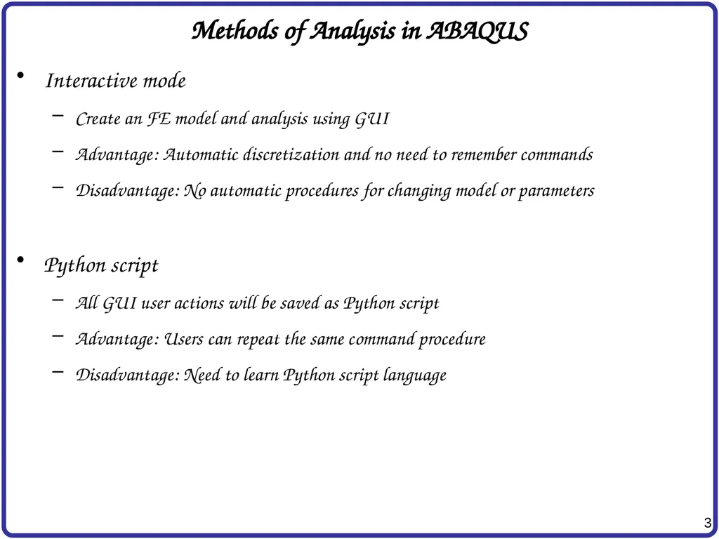
Methods of Analysis in ABAQUS Analysis input file
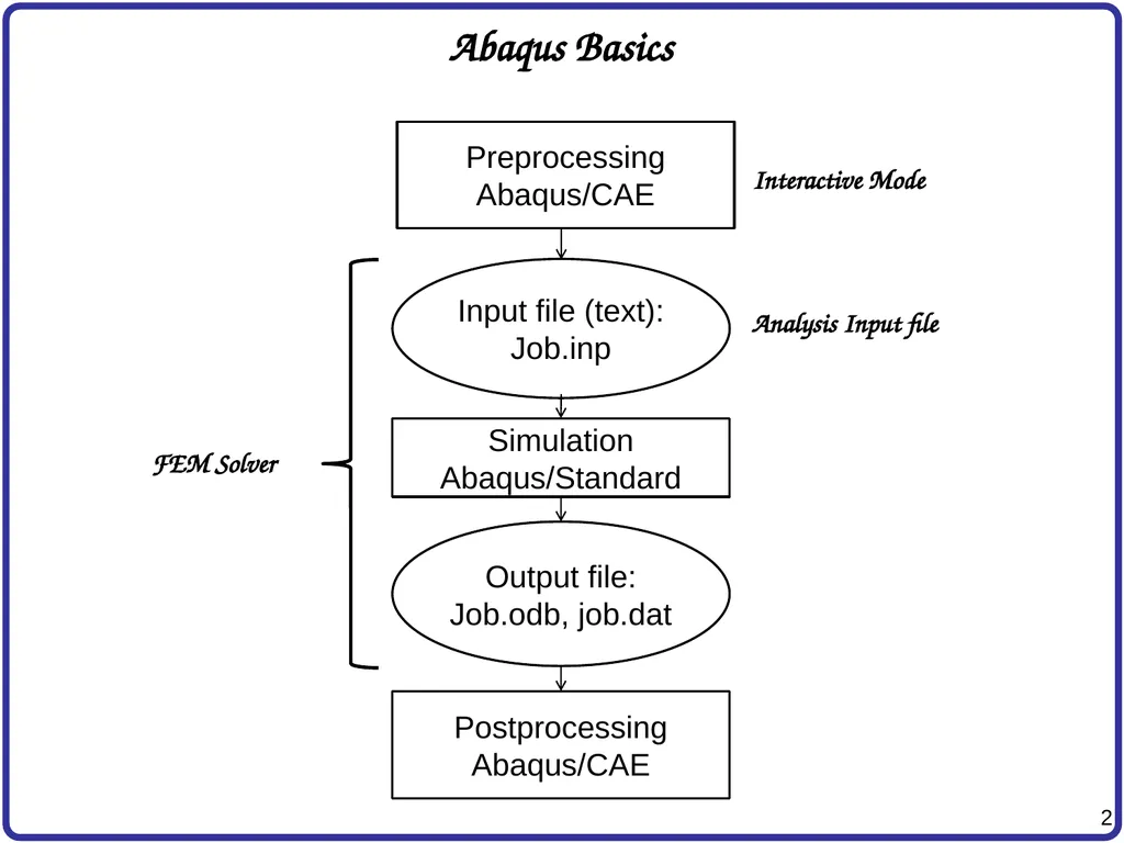
ABAQUS solver reads an analysis input file
Possible to manually create an analysis input file
Advantage: Users can change model directly without GUI
Disadvantage: Users have to discretize model and learn ABAQUS input file grammar<br>
05
Components in ABAQUS Model Geometry modeling (define geometry)
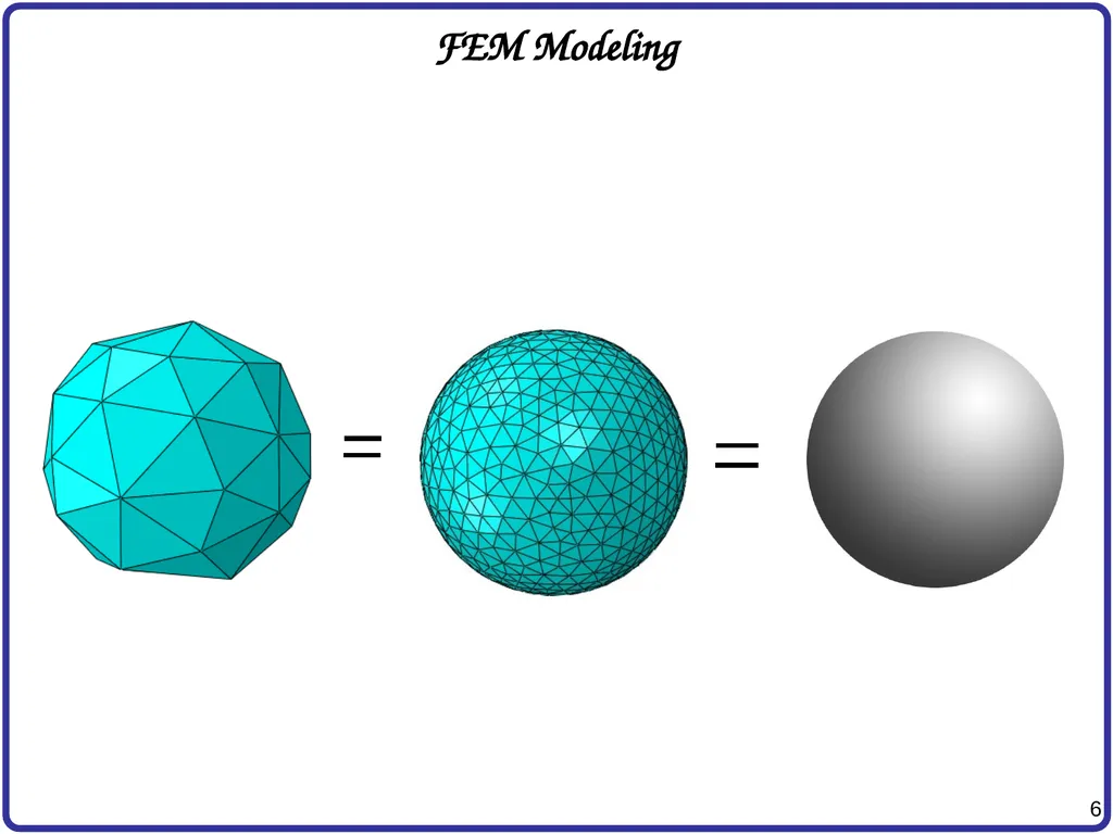
Creating nodes and elements (discretization)
Element section properties (area, moment of inertia, etc)
Material data (linear/nonlinear, elastic/plastic, isotropic/orthotropic, etc)
Loads and boundary conditions (nodal force, pressure, gravity, fixed displacement, joint, relation, etc)
Analysis type (linear/nonlinear, static/dynamic, etc)
Output requests<br>
07
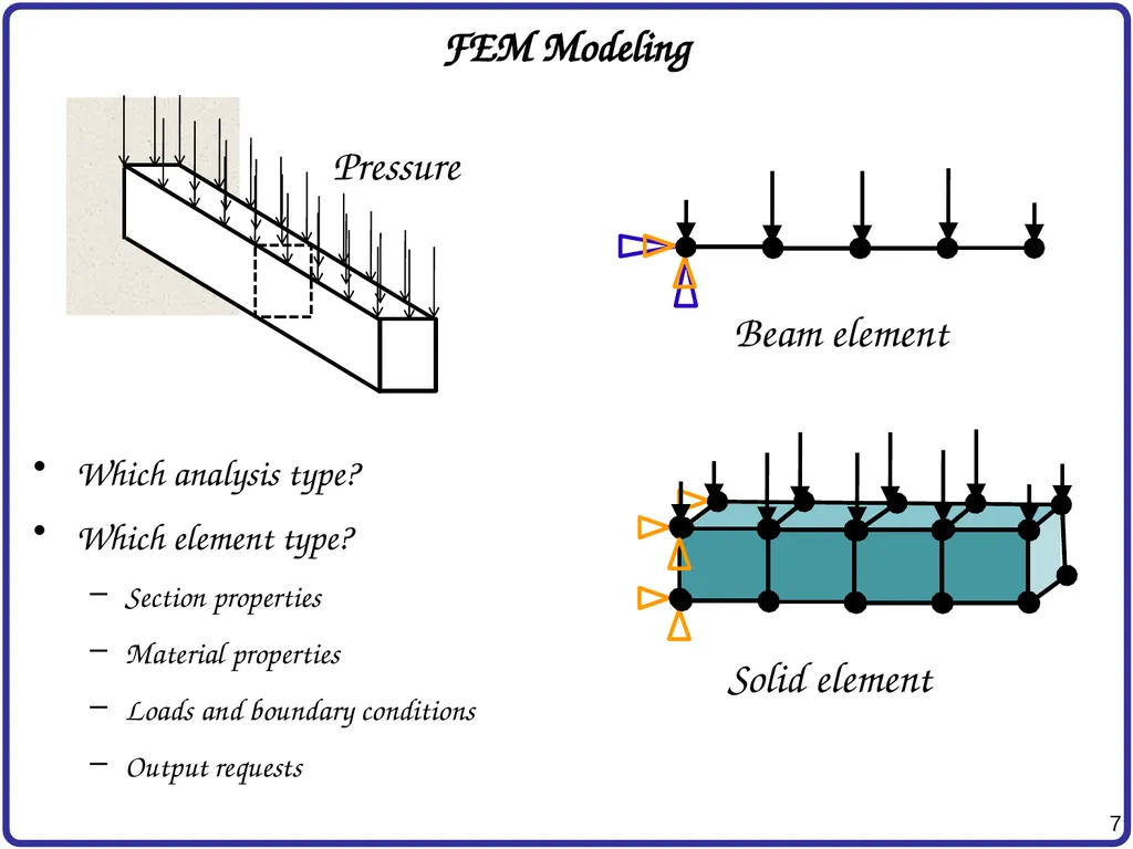
FEM Modeling Which analysis type?
Which element type?
Section properties
Material properties
Loads and boundary conditions
Output requests Beam element Solid element<br>
08
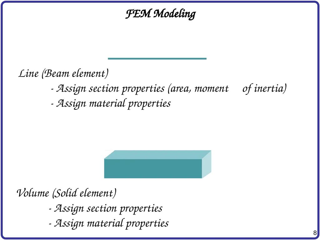
Line (Beam element)
- Assign section properties (area, moment of inertia)
- Assign material properties Volume (Solid element)
- Assign section properties
- Assign material properties FEM Modeling<br>
09
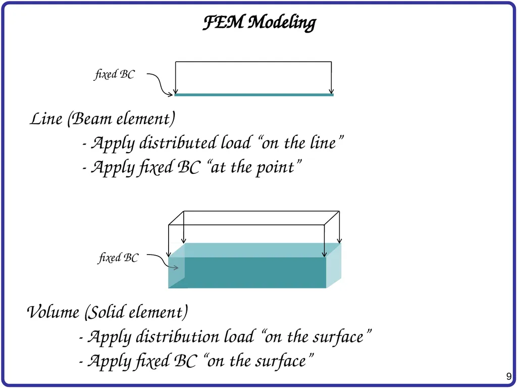
FEM Modeling Line (Beam element)
- Apply distributed load “on the line”
- Apply fixed BC “at the point” Volume (Solid element)
- Apply distribution load “on the surface”
- Apply fixed BC “on the surface” fixed BC fixed BC<br>
10
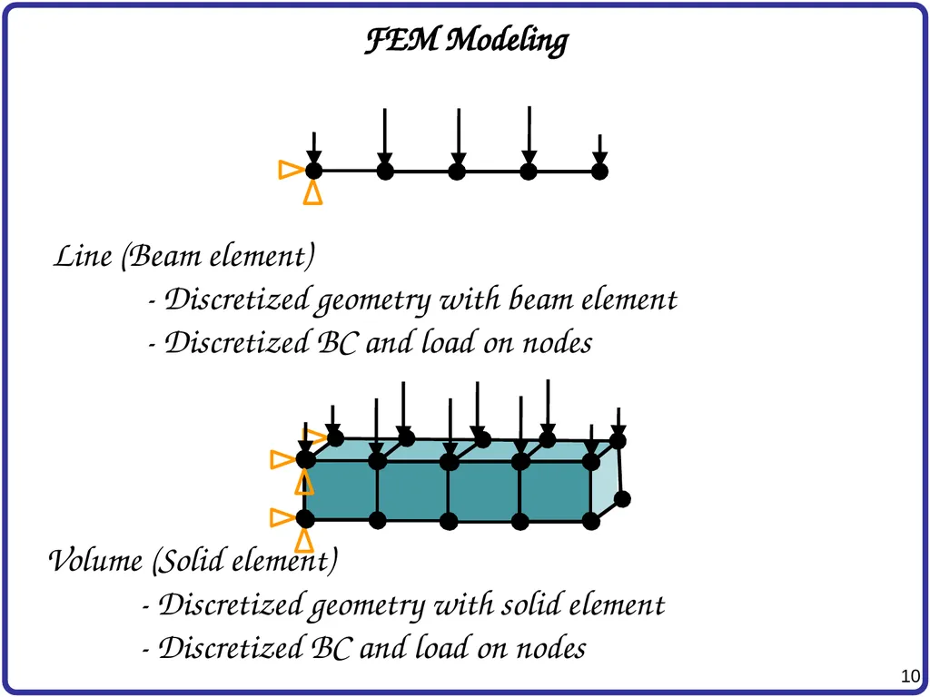
FEM Modeling Line (Beam element)
- Discretized geometry with beam element
- Discretized BC and load on nodes Volume (Solid element)
- Discretized geometry with solid element
- Discretized BC and load on nodes<br>
11
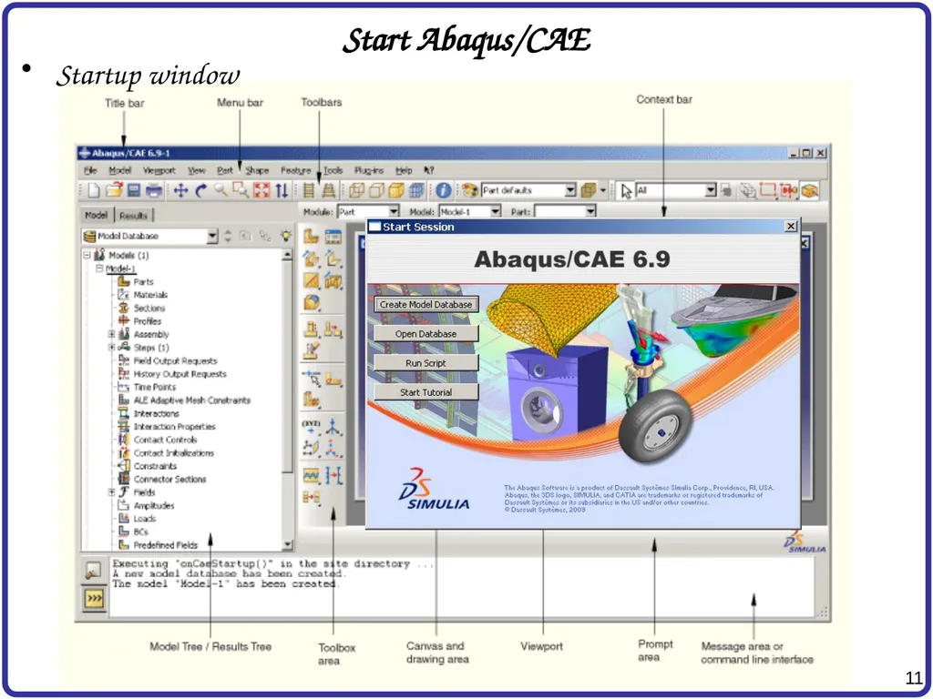
Start Abaqus/CAE Startup window<br>
12
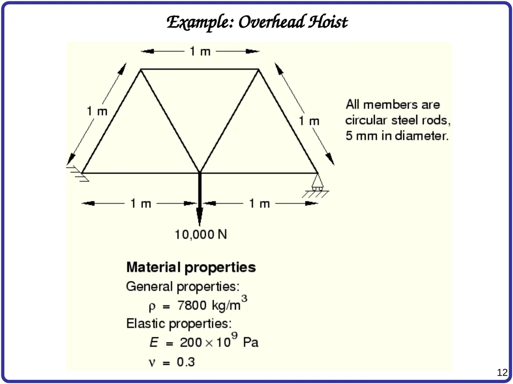
Example: Overhead Hoist<br>
13
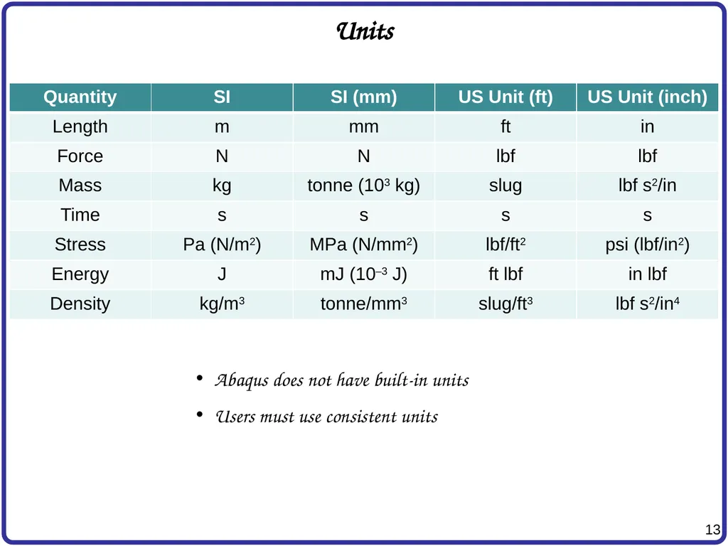
Units Abaqus does not have built-in units
Users must use consistent units<br>
14
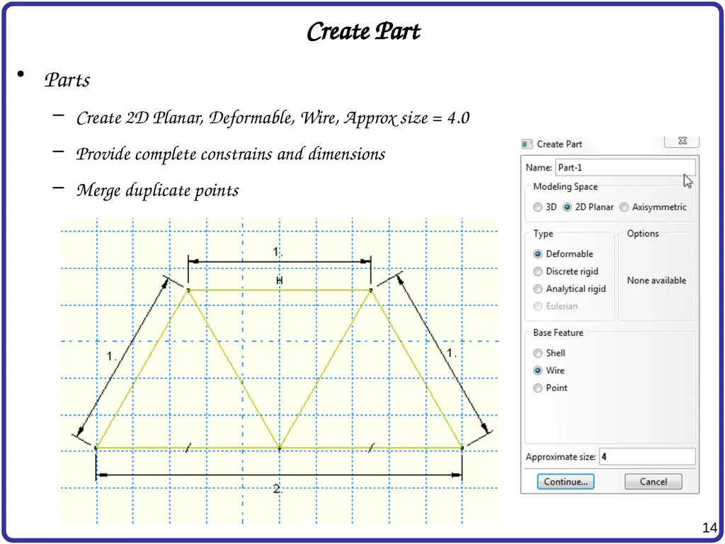
Create Part Parts
Create 2D Planar, Deformable, Wire, Approx size = 4.0
Provide complete constrains and dimensions
Merge duplicate points<br>
15
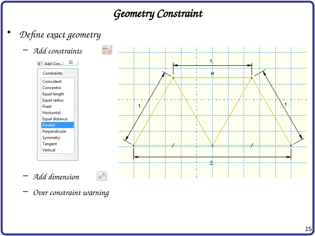
Geometry Constraint Define exact geometry
Add constraints
Add dimension
Over constraint warning<br>
16
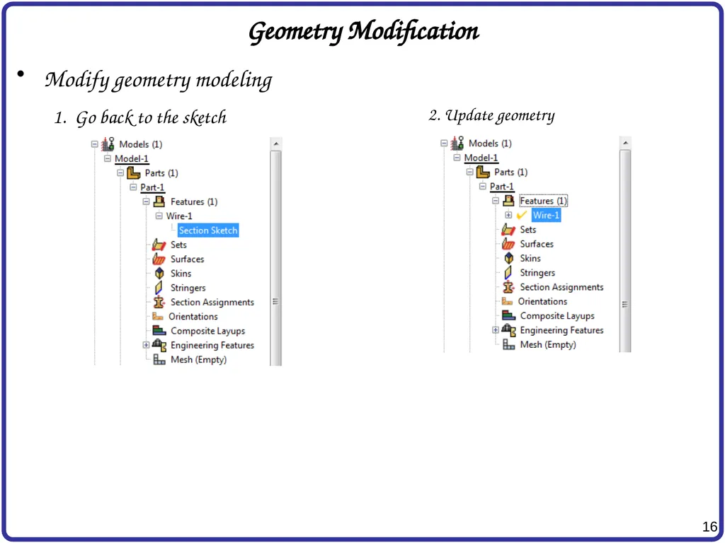
Geometry Modification Modify geometry modeling
1. Go back to the sketch 2. Update geometry<br>
17
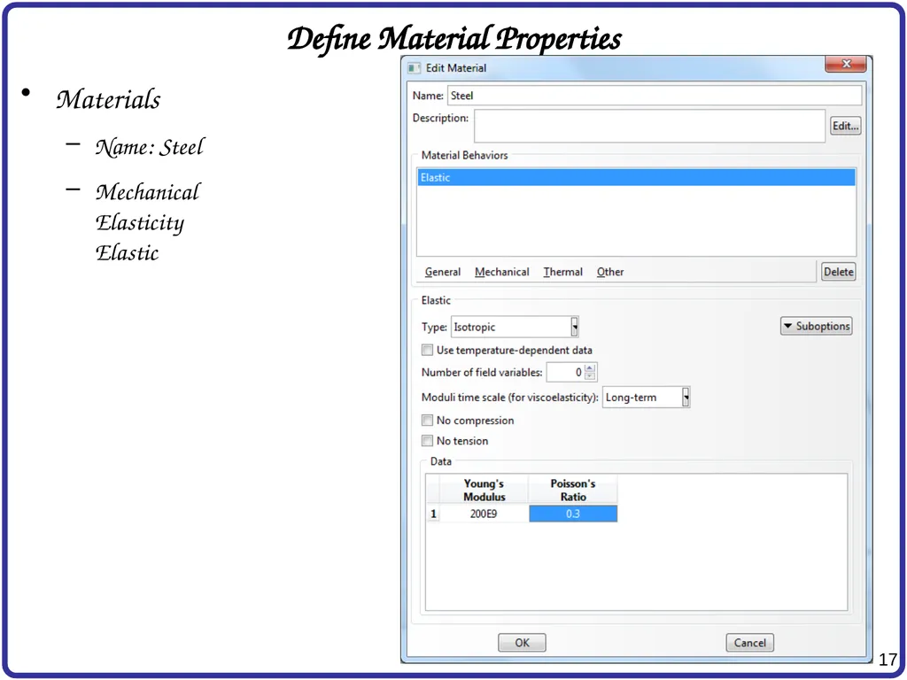
Define Material Properties Materials
Name: Steel
Mechanical�Elasticity�Elastic<br>
18
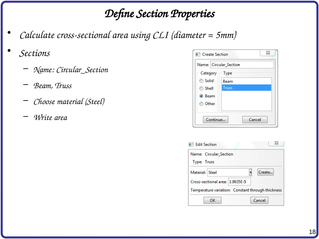
Define Section Properties Calculate cross-sectional area using CLI (diameter = 5mm)
Sections
Name: Circular_Section
Beam, Truss
Choose material (Steel)
Write area<br>
19
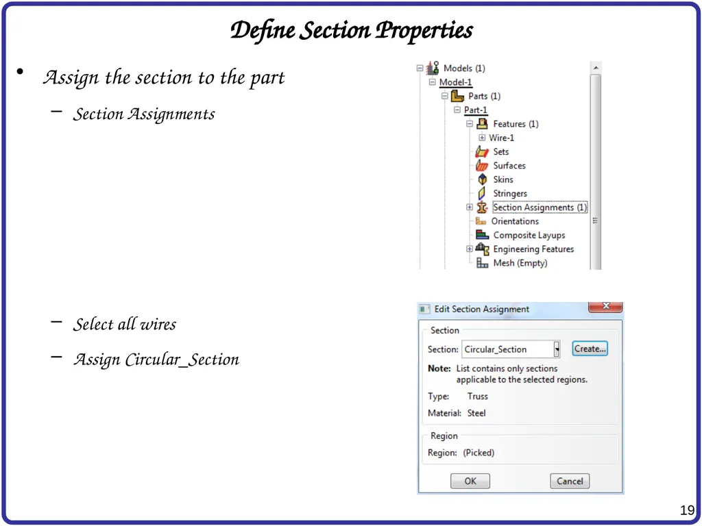
Define Section Properties Assign the section to the part
Section Assignments
Select all wires
Assign Circular_Section<br>
20
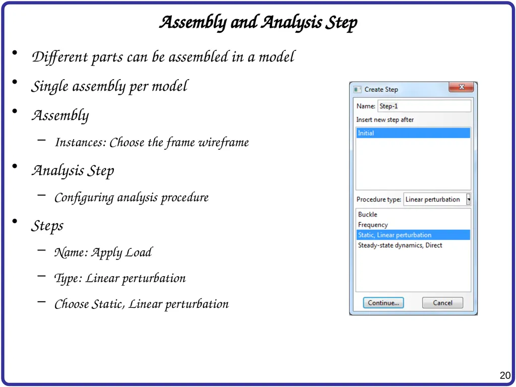
Assembly and Analysis Step Different parts can be assembled in a model
Single assembly per model
Assembly
Instances: Choose the frame wireframe
Analysis Step
Configuring analysis procedure
Steps
Name: Apply Load
Type: Linear perturbation
Choose Static, Linear perturbation<br>
21
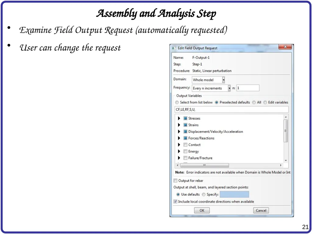
Assembly and Analysis Step Examine Field Output Request (automatically requested)
User can change the request<br>
22
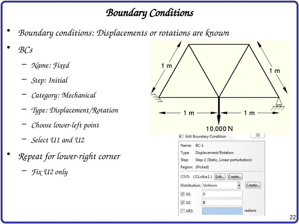
Boundary Conditions Boundary conditions: Displacements or rotations are known
BCs
Name: Fixed
Step: Initial
Category: Mechanical
Type: Displacement/Rotation
Choose lower-left point
Select U1 and U2
Repeat for lower-right corner
Fix U2 only<br>
23
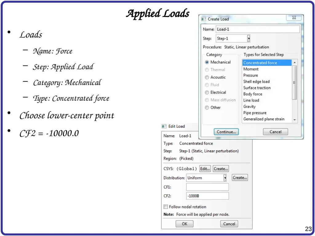
Applied Loads Loads
Name: Force
Step: Applied Load
Category: Mechanical
Type: Concentrated force
Choose lower-center point
CF2 = -10000.0<br>
24
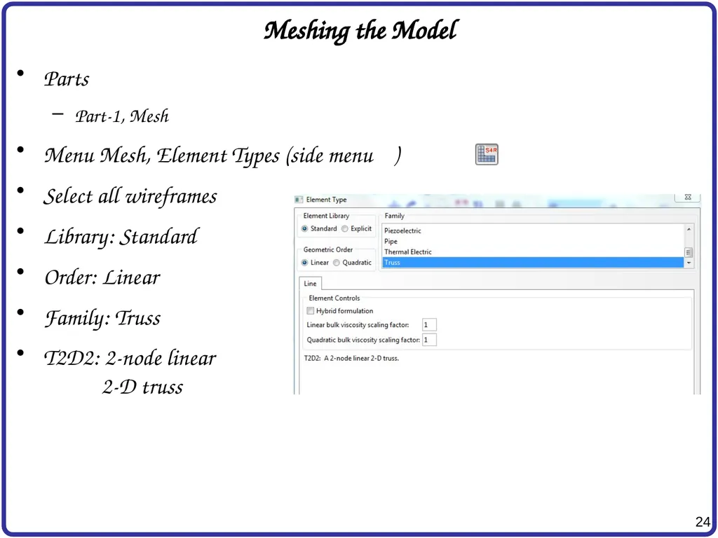
Meshing the Model Parts
Part-1, Mesh
Menu Mesh, Element Types (side menu )
Select all wireframes
Library: Standard
Order: Linear
Family: Truss
T2D2: 2-node linear� 2-D truss<br>
25
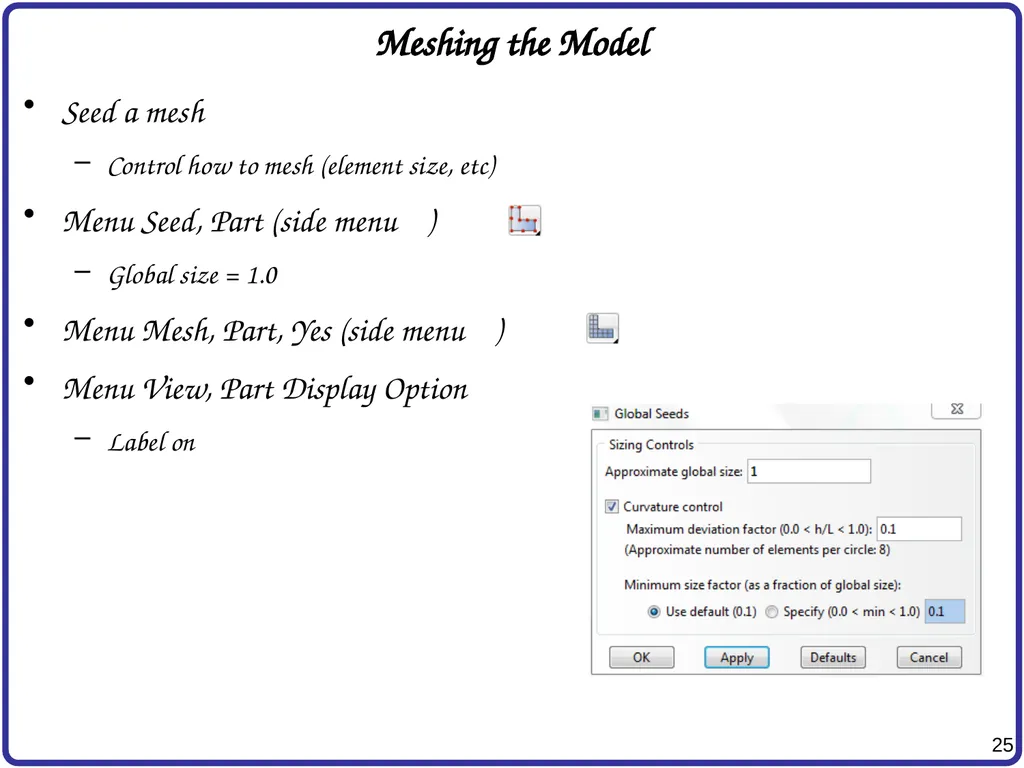
Meshing the Model Seed a mesh
Control how to mesh (element size, etc)
Menu Seed, Part (side menu )
Global size = 1.0
Menu Mesh, Part, Yes (side menu )
Menu View, Part Display Option
Label on<br>
26
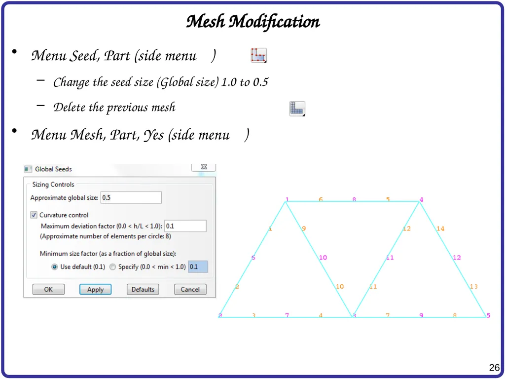
Mesh Modification Menu Seed, Part (side menu )
Change the seed size (Global size) 1.0 to 0.5
Delete the previous mesh
Menu Mesh, Part, Yes (side menu )<br>
27
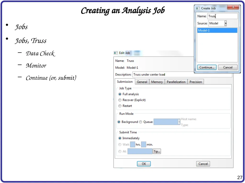
Creating an Analysis Job Jobs
Jobs, Truss
Data Check
Monitor
Continue (or, submit)<br>
28
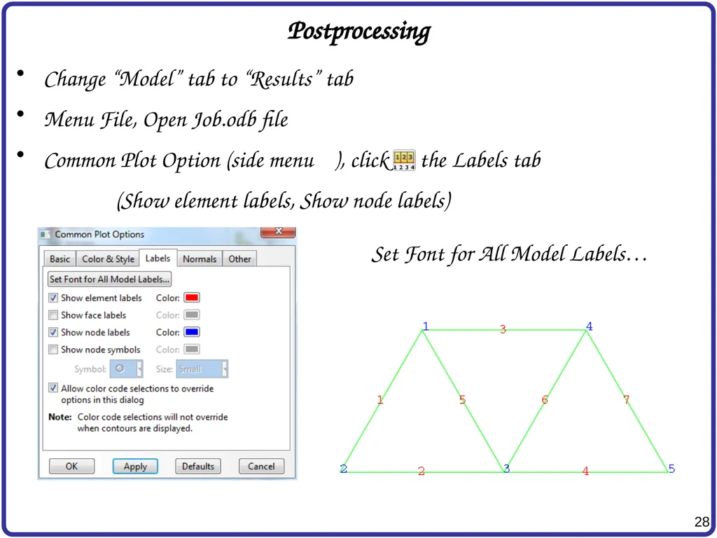
Postprocessing Change “Model” tab to “Results” tab
Menu File, Open Job.odb file
Common Plot Option (side menu ), click on the Labels tab
(Show element labels, Show node labels) Set Font for All Model Labels…<br>
29
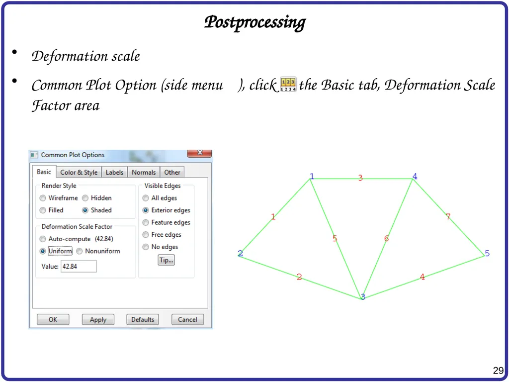
Postprocessing Deformation scale
Common Plot Option (side menu ), click on the Basic tab, Deformation Scale Factor area<br>
30
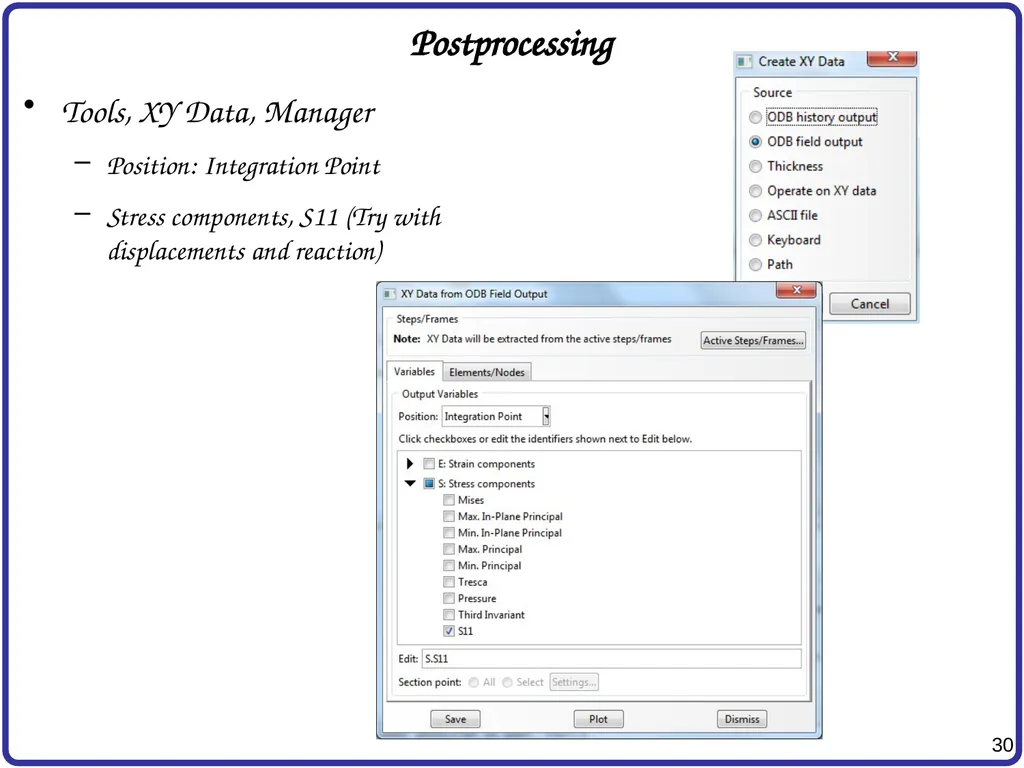
Postprocessing Tools, XY Data, Manager
Position: Integration Point
Stress components, S11 (Try with displacements and reaction)<br>
31
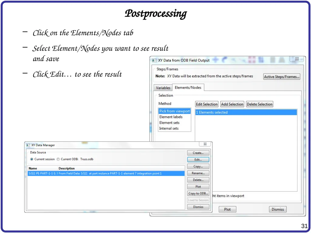
Postprocessing Click on the Elements/Nodes tab
Select Element/Nodes you want to see result and save
Click Edit… to see the result<br>
32
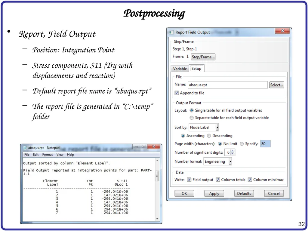
Postprocessing Report, Field Output
Position: Integration Point
Stress components, S11 (Try with displacements and reaction)
Default report file name is “abaqus.rpt”
The report file is generated in “C:\temp” folder<br>
33
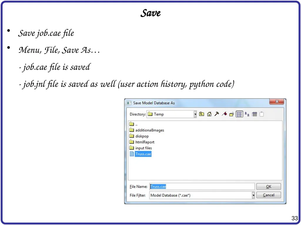
Save Save job.cae file
Menu, File, Save As…
- job.cae file is saved
- job.jnl file is saved as well (user action history, python code)<br>