Fluvial Hydraulics CH-6 Bed-Load Transport

slide1. Fluvial HydraulicsCH-6 Bed-Load Transport<br>
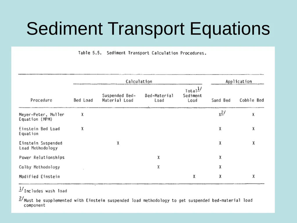
slide2. Sediment Transport Equations Sediment transport equations used to determine CAPACITY for set of flow conditions
Capacity needed for many different analyses such as aggradation/degradation, general scour/deposition, and lateral migration
First step is to select appropriate equation:
Predicated on an understanding of the system being studied
Some formulas developed for sand-bed streams with high suspended load transport
Other equations pertain to conditions where bed-load transport dominates
Study objectives determine the portion of the sediment transport that needs to be estimated and the level of accuracy
Some formulas independently predict bed load and suspended load
Other formulas estimated bed-material load (i.e., bed load + suspended load) – usually these equations do not include wash load
Procedures exist that incorporate sediment sampling data, such as the modified Einstein procedure, that can estimate total sediment transport rate (including wash load)<br>
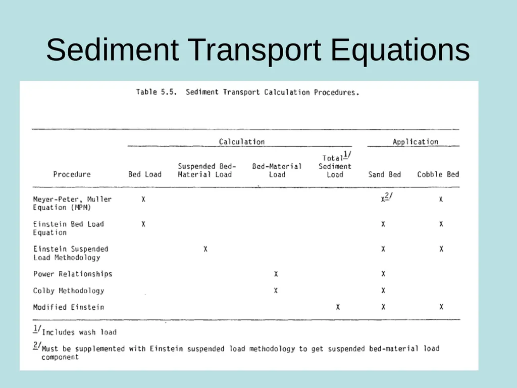
slide3. Sediment Transport Equations<br>
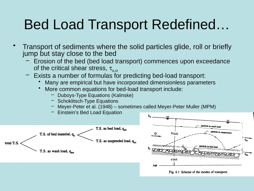
slide4. Bed Load Transport Redefined… Transport of sediments where the solid particles glide, roll or briefly jump but stay close to the bed
Erosion of the bed (bed load transport) commences upon exceedance of the critical shear stress, to,cr
Exists a number of formulas for predicting bed-load transport:
Many are empirical but have incorporated dimensionless parameters
More common equations for bed-load transport include:
Duboys-Type Equations (Kalinske)
Schoklitsch-Type Equations
Meyer-Peter et al. (1948) – sometimes called Meyer-Peter Muller (MPM)
Einstein’s Bed Load Equation<br>
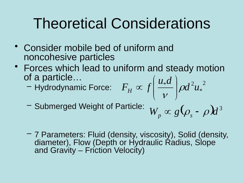
slide5. Theoretical Considerations Consider mobile bed of uniform and noncohesive particles
Forces which lead to uniform and steady motion of a particle…
Hydrodynamic Force:

Submerged Weight of Particle:

7 Parameters: Fluid (density, viscosity), Solid (density, diameter), Flow (Depth or Hydraulic Radius, Slope and Gravity – Friction Velocity)<br>
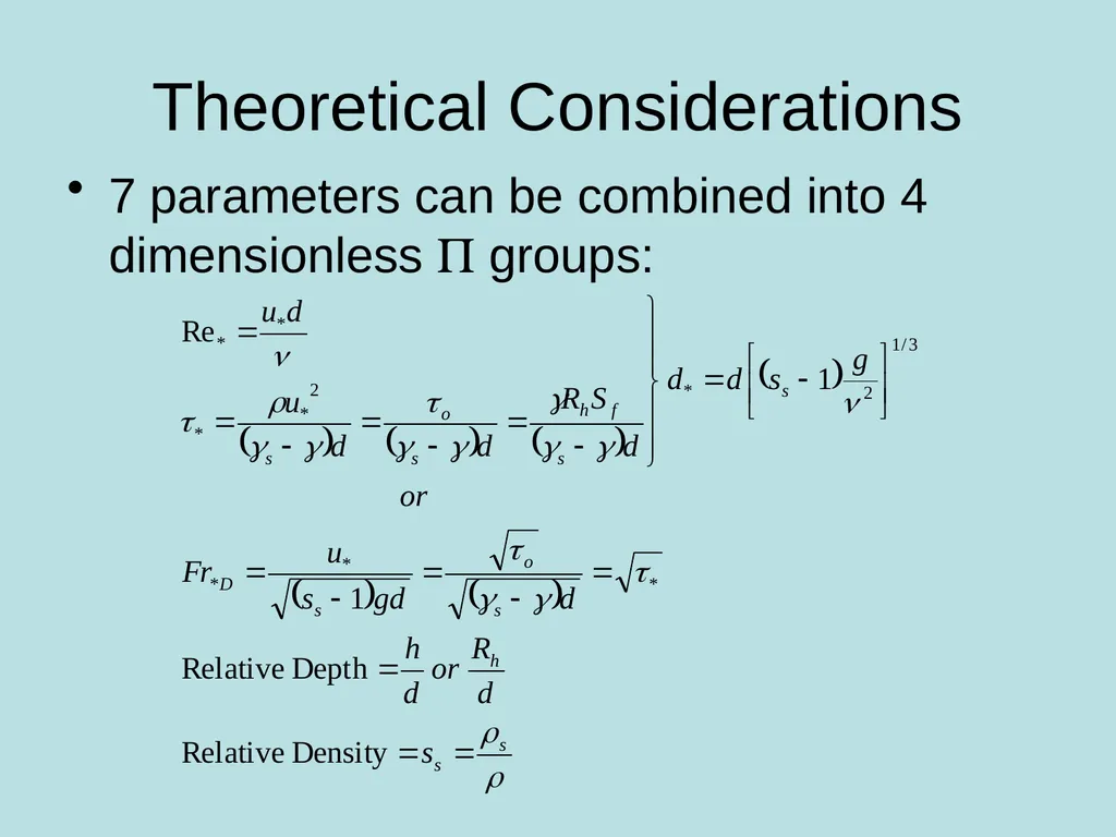
slide6. Theoretical Considerations 7 parameters can be combined into 4 dimensionless P groups:<br>
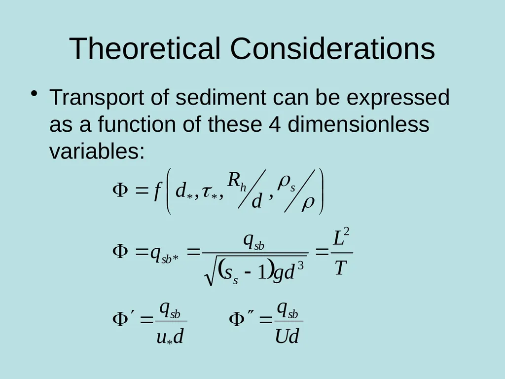
slide7. Theoretical Considerations Transport of sediment can be expressed as a function of these 4 dimensionless variables:<br>
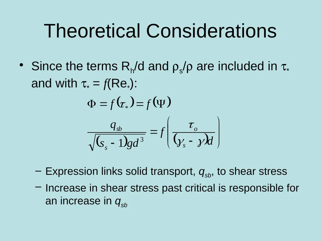
slide8. Theoretical Considerations Since the terms Rh/d and rs/r are included in t* and with t* = f(Re*):

Expression links solid transport, qsb, to shear stress
Increase in shear stress past critical is responsible for an increase in qsb<br>
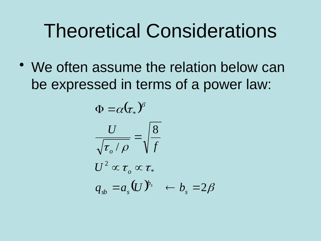
slide9. Theoretical Considerations We often assume the relation below can be expressed in terms of a power law:<br>
slide10. Bed-Load Transport Equations Be Careful!!!
Formulas give “reasonably satisfying results” with the parameter domain for which they were derived
Application of formulas should be done with great care!<br>
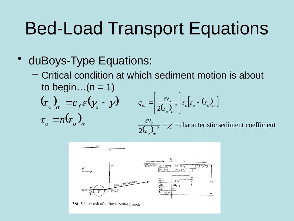
slide11. Bed-Load Transport Equations duBoys-Type Equations:
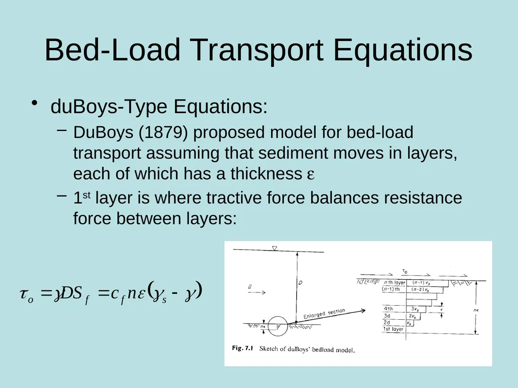
DuBoys (1879) proposed model for bed-load transport assuming that sediment moves in layers, each of which has a thickness e
1st layer is where tractive force balances resistance force between layers:<br>
slide12. Bed-Load Transport Equations duBoys-Type Equations:
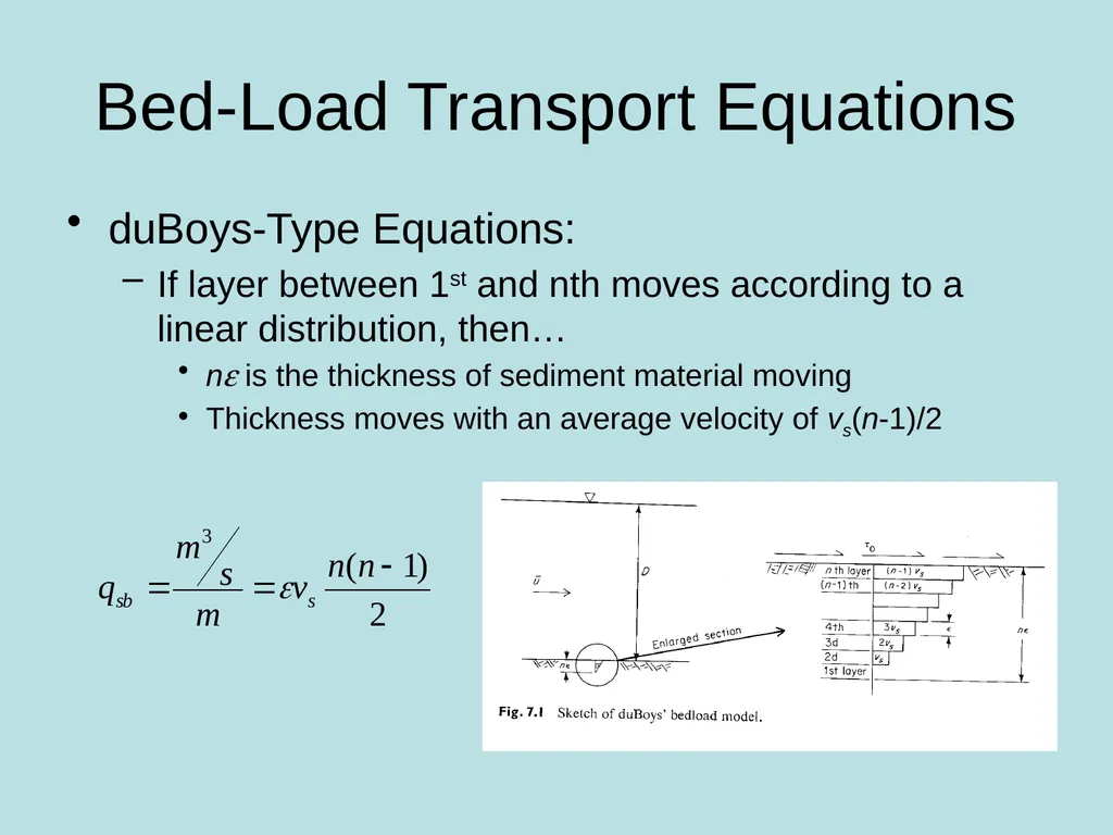
If layer between 1st and nth moves according to a linear distribution, then…
ne is the thickness of sediment material moving
Thickness moves with an average velocity of vs(n-1)/2<br>
slide13. Bed-Load Transport Equations duBoys-Type Equations:
Critical condition at which sediment motion is about to begin…(n = 1)<br>
slide14. Bed-Load Transport Equations duBoys-Type Equations:
Assumptions of this equation have been shown to disagree totally with observations of bed-load transport
Bed load does not move as sliding layers (Schoklitsch, 1914)
However, there is generally good agreement between this equation and field/laboratory data
Proper use of the equation depends on correct evaluation of the characteristic sediment coefficient, c

Sidenote: generally all bed load equations based on excess shear stress are classified as duBoys-type equations<br>
slide15. Bed-Load Transport Equations duBoys-Type Equations:
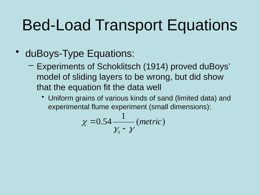
Experiments of Schoklitsch (1914) proved duBoys’ model of sliding layers to be wrong, but did show that the equation fit the data well
Uniform grains of various kinds of sand (limited data) and experimental flume experiment (small dimensions):<br>
slide16. Bed-Load Transport Equations duBoys-Type Equations:
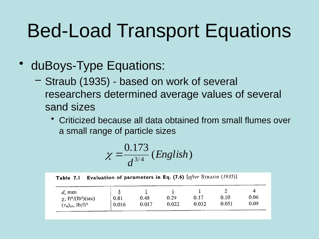
Straub (1935) - based on work of several researchers determined average values of several sand sizes
Criticized because all data obtained from small flumes over a small range of particle sizes<br>
slide17. Bed-Load Transport Equations duBoys-Type Equations:
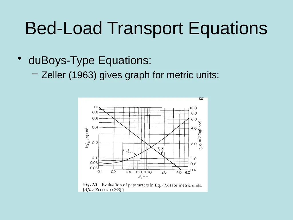
Zeller (1963) gives graph for metric units:<br>
slide18. Bed-Load Transport Equations duBoys-Type Equations:
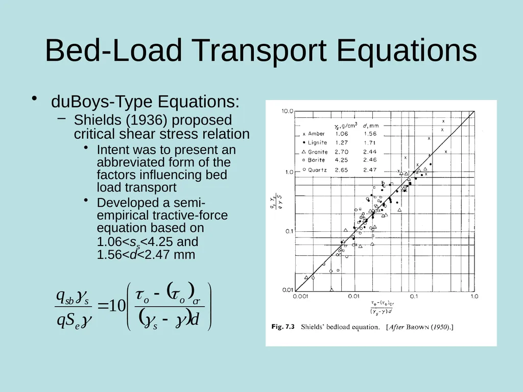
Shields (1936) proposed critical shear stress relation
Intent was to present an abbreviated form of the factors influencing bed load transport
Developed a semi-empirical tractive-force equation based on 1.06<ss<4.25 and 1.56<d<2.47 mm<br>
slide19. Bed-Load Transport Equations duBoys-Type Equations:
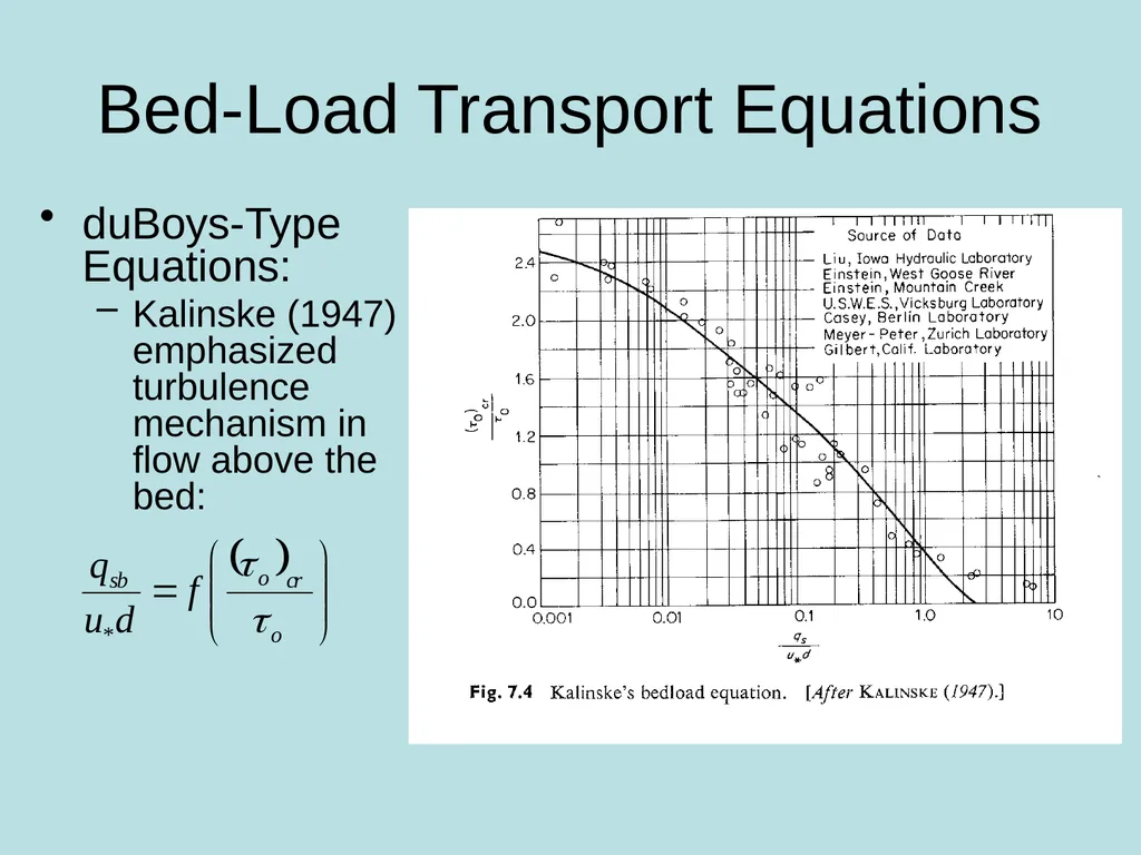
Kalinske (1947) emphasized turbulence mechanism in flow above the bed:<br>
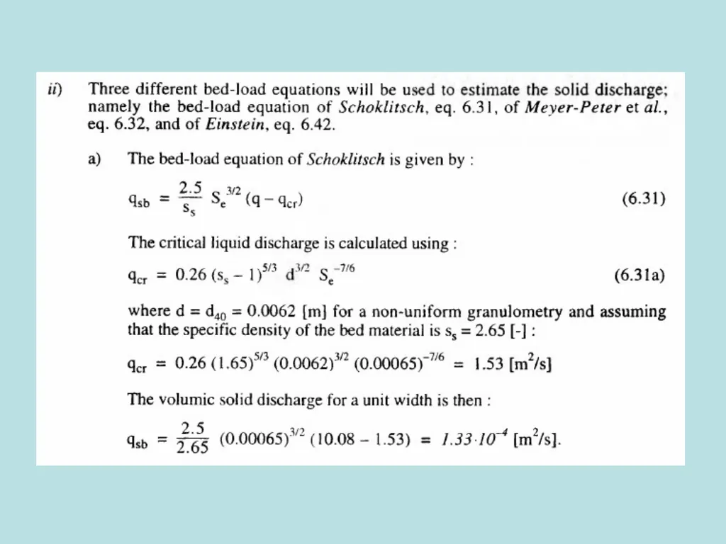
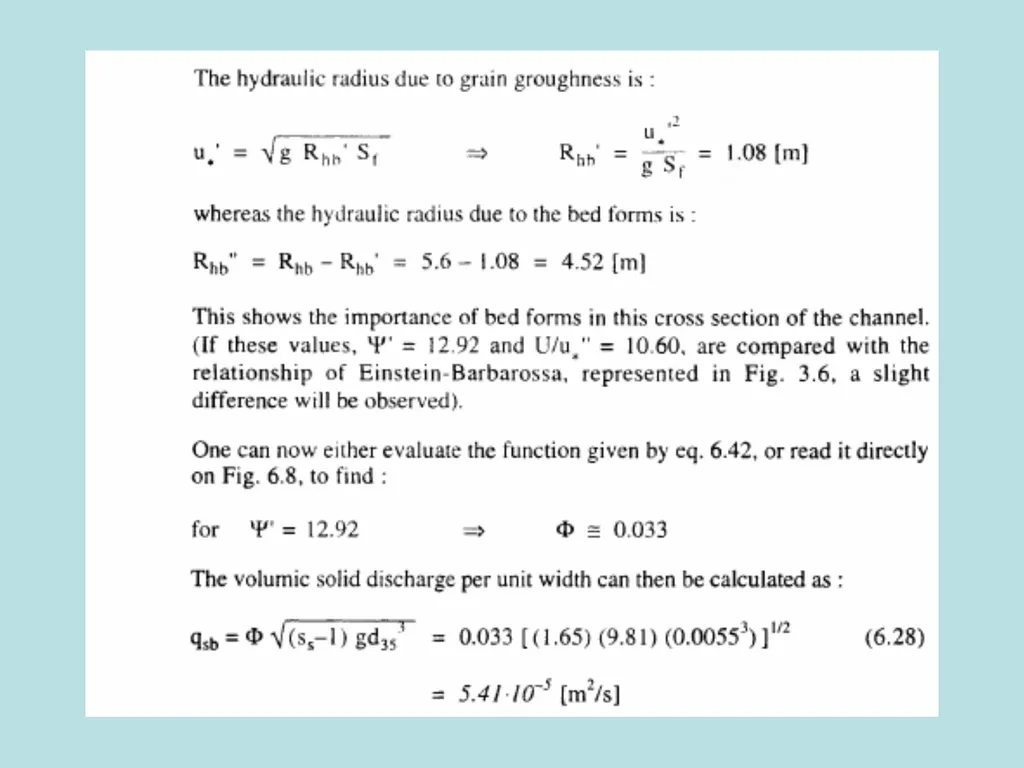
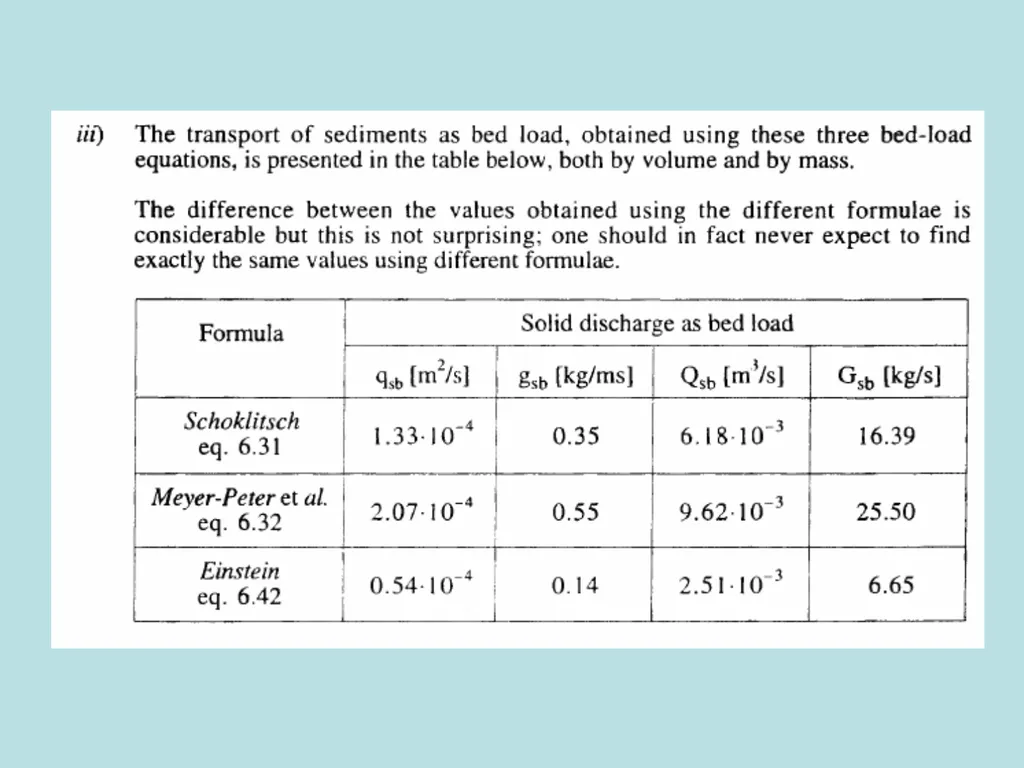
slide20. Example – Graf 6.D An artificial channel has been constructed to divert a certain discharge from a river. This channel has an approximately rectangular cross-section with a width of B = 46.5 m and a bed slope of Sf=6.5 x 10-4. Uniform flow is established when the flow depth is 5.6 m. Velocity-profile measurements suggest an average velocity of 1.8 m/s and n’ = 0.0212 (due to bed roughness). Estimate the bed-load transport using the Kalinske equation. Express the solid discharge as a concentration.<br>
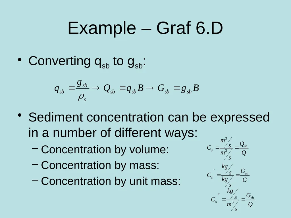
slide21. Example – Graf 6.D Converting qsb to gsb:

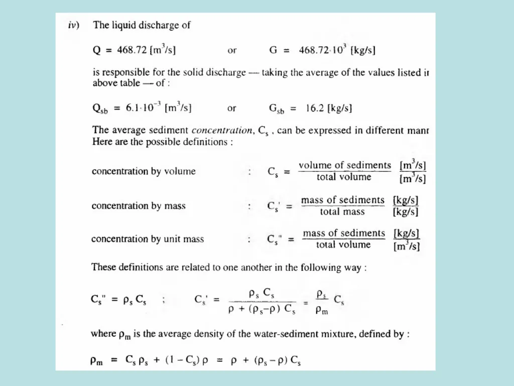
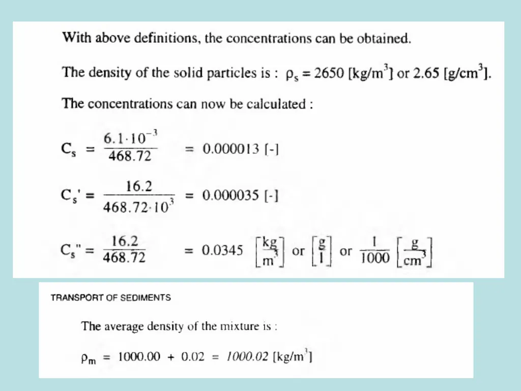
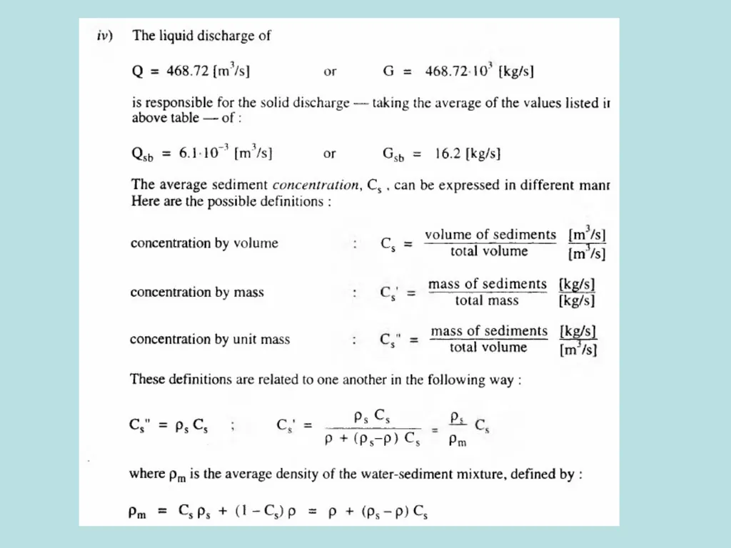
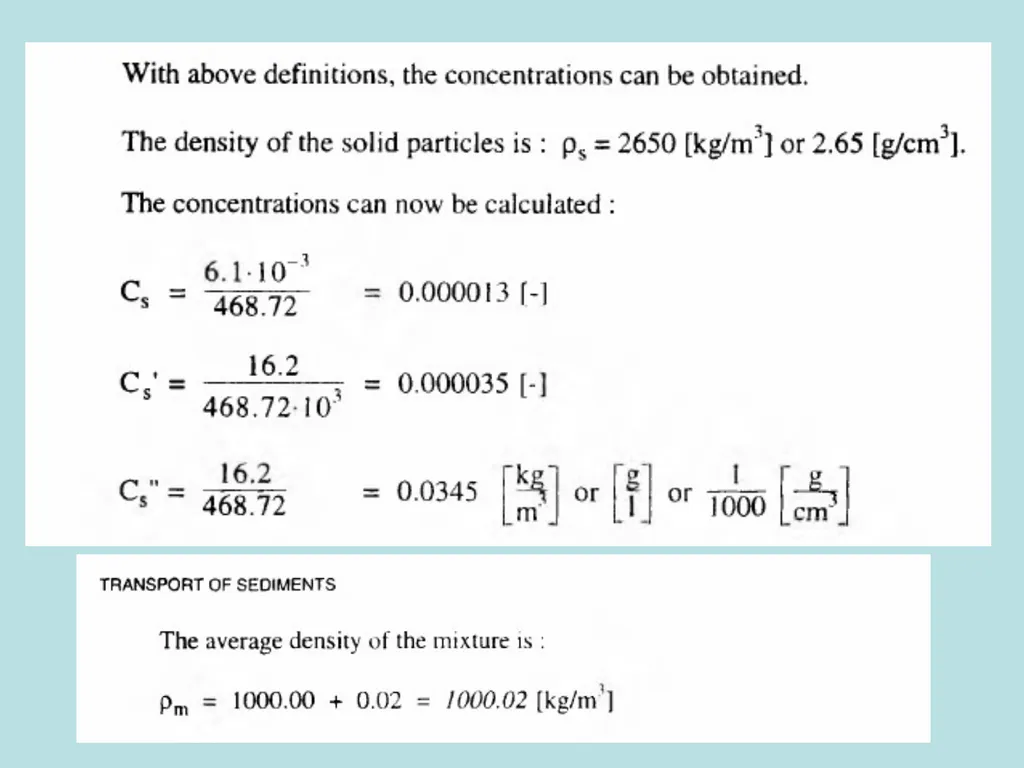
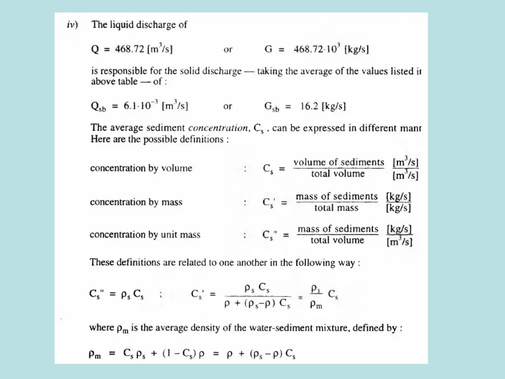
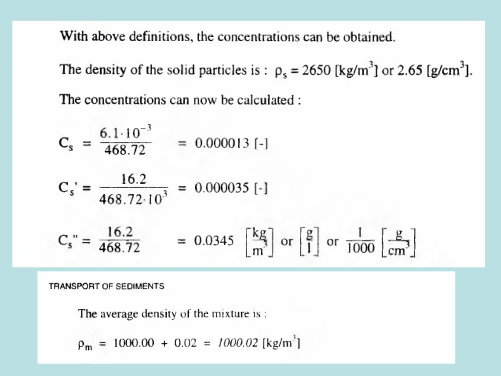
Sediment concentration can be expressed in a number of different ways:
Concentration by volume:
Concentration by mass:
Concentration by unit mass:<br>
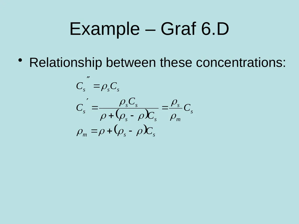
slide22. Example – Graf 6.D Relationship between these concentrations:<br>
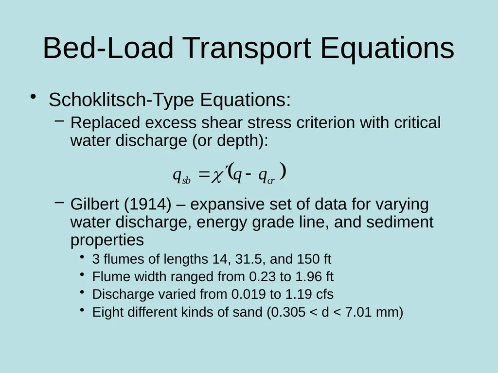
slide23. Bed-Load Transport Equations Schoklitsch-Type Equations:
Replaced excess shear stress criterion with critical water discharge (or depth):

Gilbert (1914) – expansive set of data for varying water discharge, energy grade line, and sediment properties
3 flumes of lengths 14, 31.5, and 150 ft
Flume width ranged from 0.23 to 1.96 ft
Discharge varied from 0.019 to 1.19 cfs
Eight different kinds of sand (0.305 < d < 7.01 mm)<br>
slide24. Bed-Load Transport Equations Schoklitsch-Type Equations:
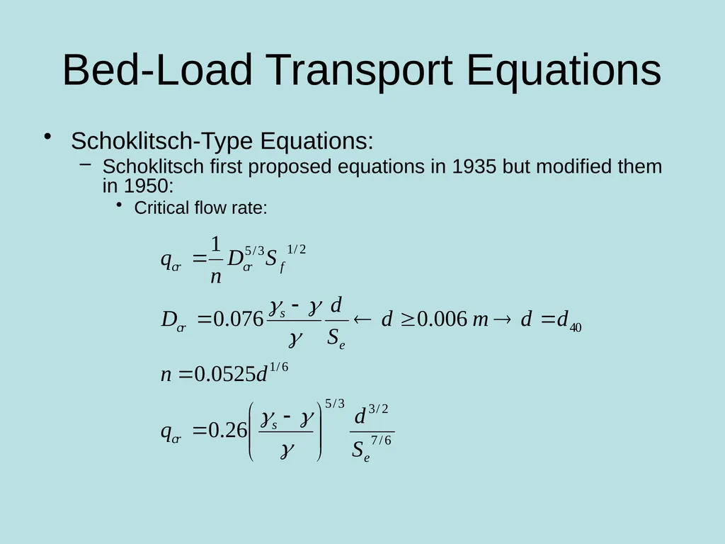
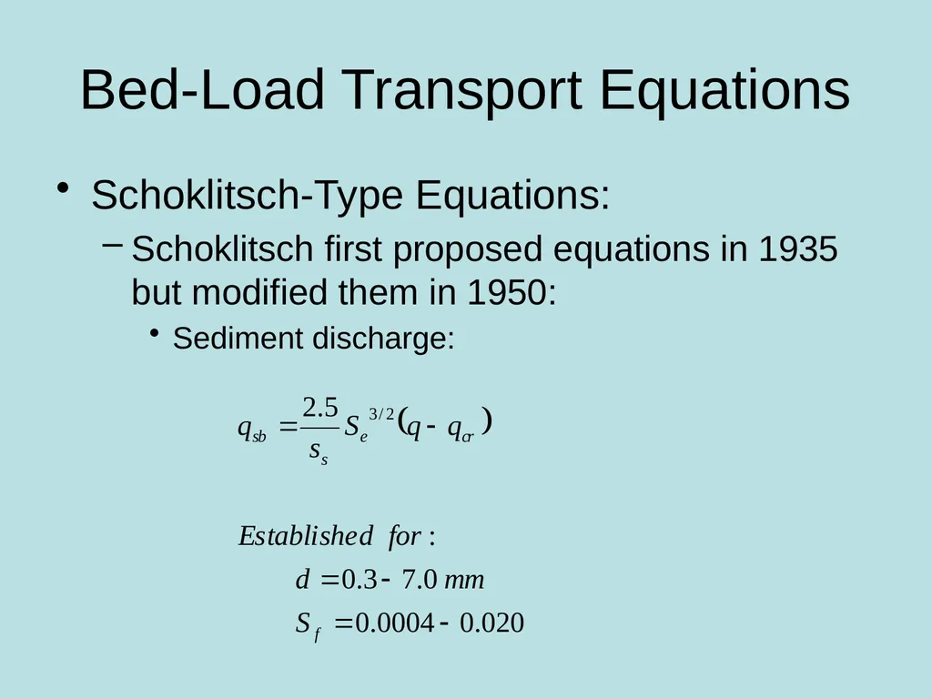
Schoklitsch first proposed equations in 1935 but modified them in 1950:
Critical flow rate:<br>
slide25. Bed-Load Transport Equations Schoklitsch-Type Equations:
Schoklitsch first proposed equations in 1935 but modified them in 1950:
Sediment discharge:<br>
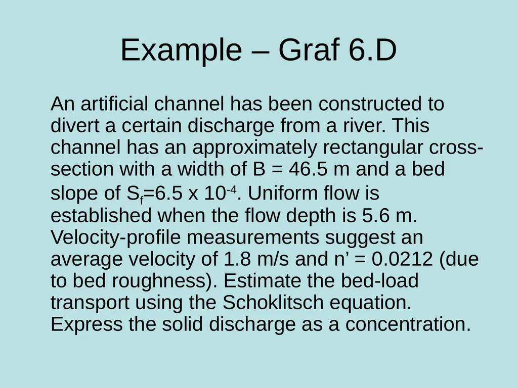
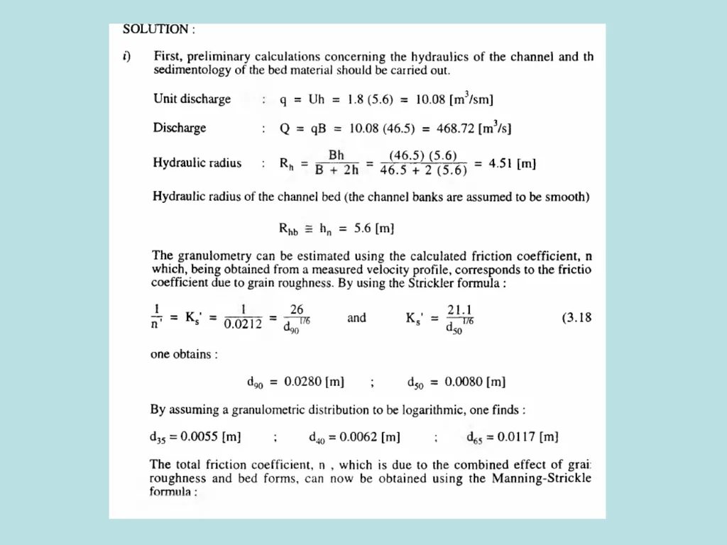
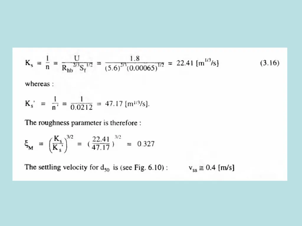
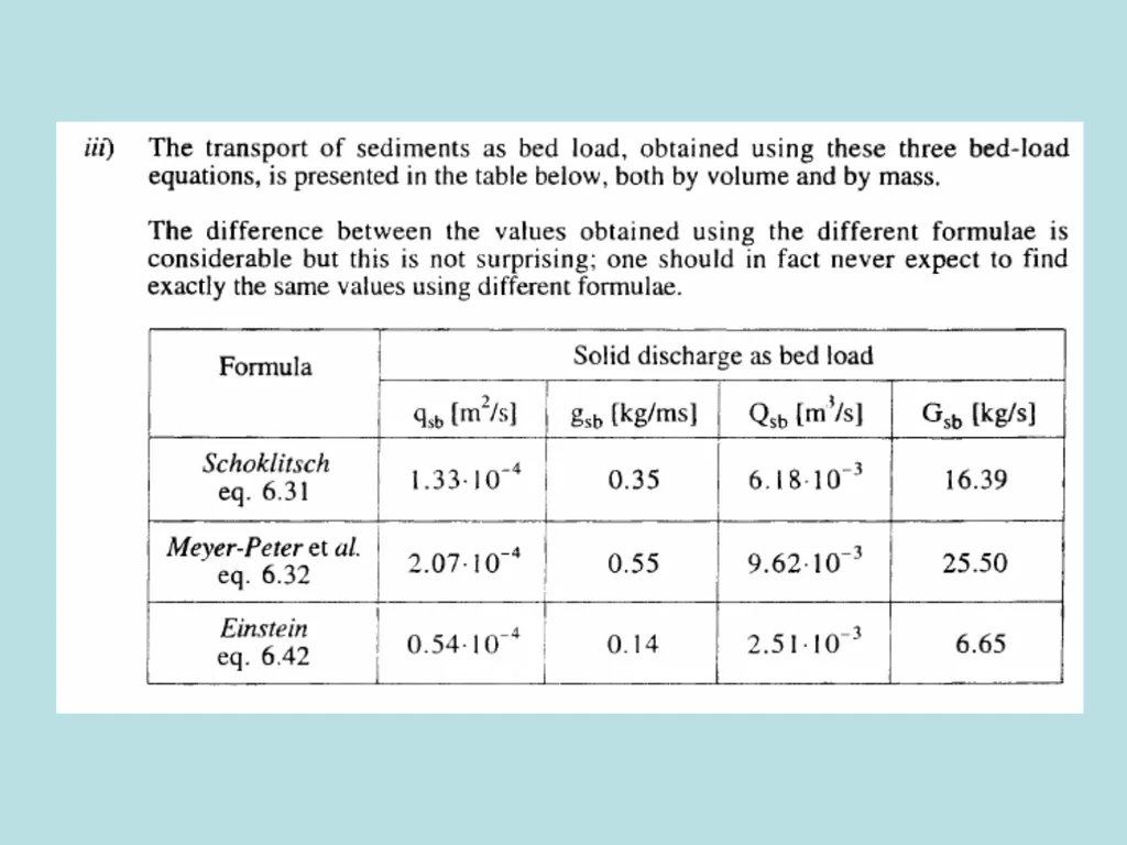
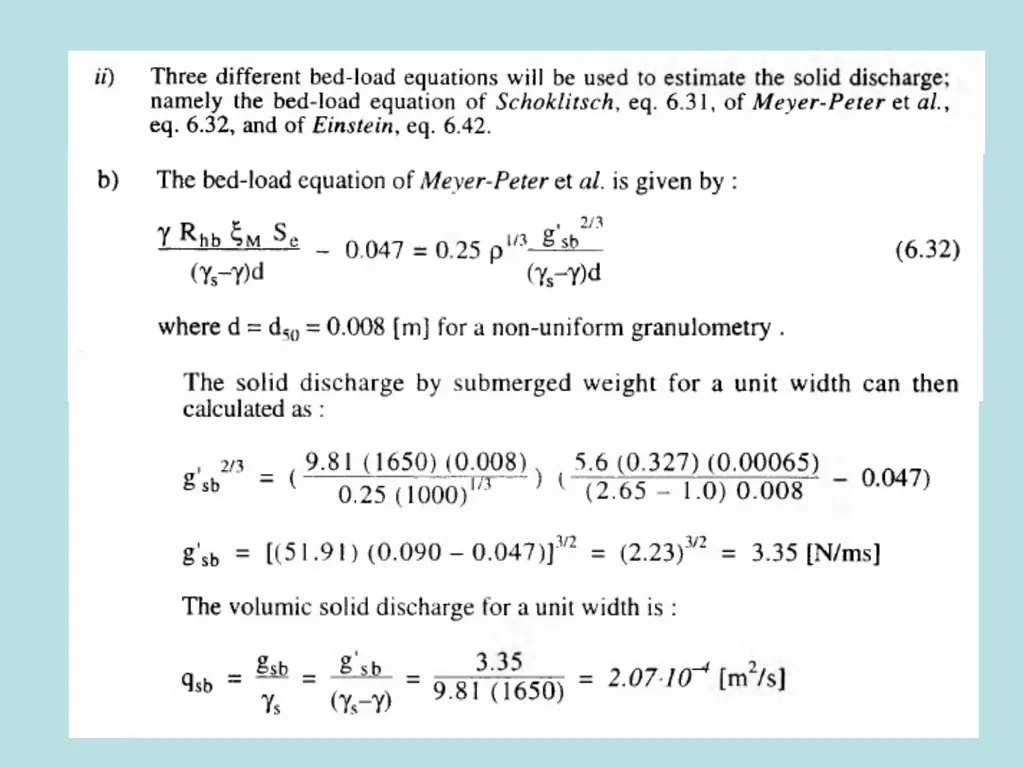
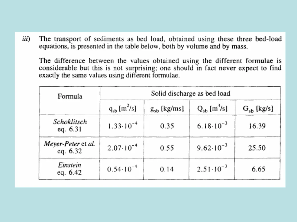
slide26. Example – Graf 6.D An artificial channel has been constructed to divert a certain discharge from a river. This channel has an approximately rectangular cross-section with a width of B = 46.5 m and a bed slope of Sf=6.5 x 10-4. Uniform flow is established when the flow depth is 5.6 m. Velocity-profile measurements suggest an average velocity of 1.8 m/s and n’ = 0.0212 (due to bed roughness). Estimate the bed-load transport using the Schoklitsch equation. Express the solid discharge as a concentration.<br>
slide33. Bed-Load Transport Equations Meyer-Peter Muller (MPM):
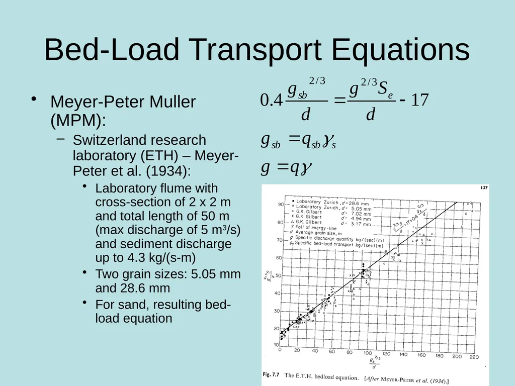
Switzerland research laboratory (ETH) – Meyer-Peter et al. (1934):
Laboratory flume with cross-section of 2 x 2 m and total length of 50 m (max discharge of 5 m3/s) and sediment discharge up to 4.3 kg/(s-m)
Two grain sizes: 5.05 mm and 28.6 mm
For sand, resulting bed-load equation<br>
slide34. Bed-Load Transport Equations Meyer-Peter Muller (MPM):
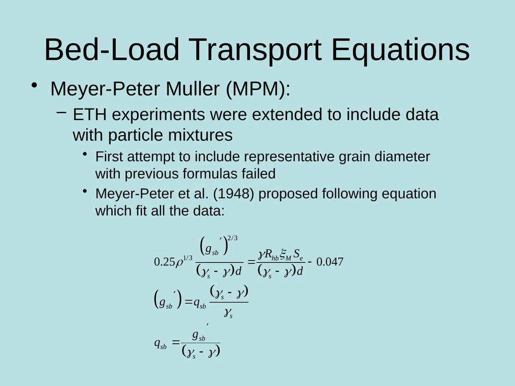
ETH experiments were extended to include data with particle mixtures
First attempt to include representative grain diameter with previous formulas failed
Meyer-Peter et al. (1948) proposed following equation which fit all the data:<br>
slide35. Bed-Load Transport Equations Meyer-Peter Muller (MPM):
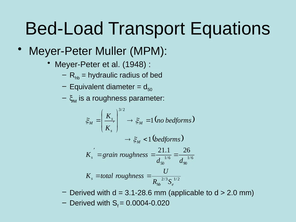
Meyer-Peter et al. (1948) :
Rhb = hydraulic radius of bed
Equivalent diameter = d50
xM is a roughness parameter:

Derived with d = 3.1-28.6 mm (applicable to d > 2.0 mm)
Derived with Sf = 0.0004-0.020<br>
slide36. Example – Graf 6.D An artificial channel has been constructed to divert a certain discharge from a river. This channel has an approximately rectangular cross-section with a width of B = 46.5 m and a bed slope of Sf=6.5 x 10-4. Uniform flow is established when the flow depth is 5.6 m. Velocity-profile measurements suggest an average velocity of 1.8 m/s and n’ = 0.0212 (due to bed roughness). Estimate the bed-load transport using the Meyer-Peter et al. formulas. Express the solid discharge as a concentration.<br>
slide41. Sediment Transport Equations<br>
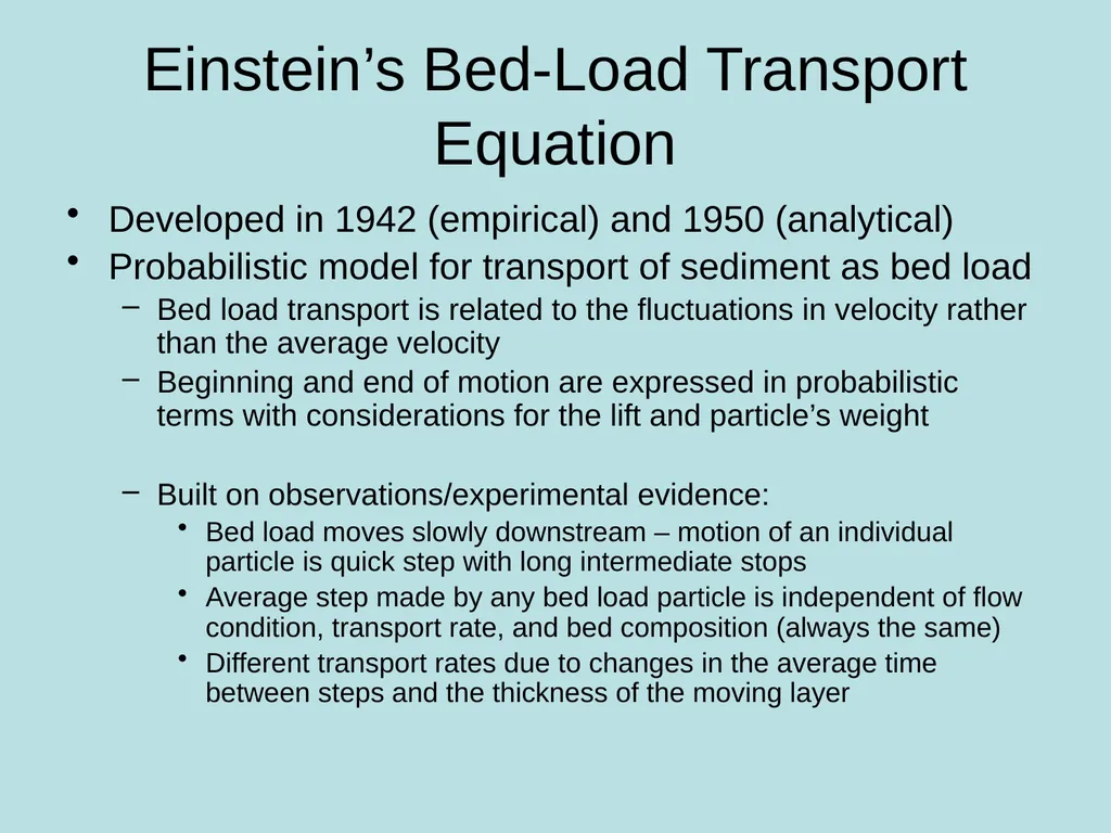
slide42. Einstein’s Bed-Load Transport Equation Developed in 1942 (empirical) and 1950 (analytical)
Probabilistic model for transport of sediment as bed load
Bed load transport is related to the fluctuations in velocity rather than the average velocity
Beginning and end of motion are expressed in probabilistic terms with considerations for the lift and particle’s weight

Built on observations/experimental evidence:
Bed load moves slowly downstream – motion of an individual particle is quick step with long intermediate stops
Average step made by any bed load particle is independent of flow condition, transport rate, and bed composition (always the same)
Different transport rates due to changes in the average time between steps and the thickness of the moving layer<br>
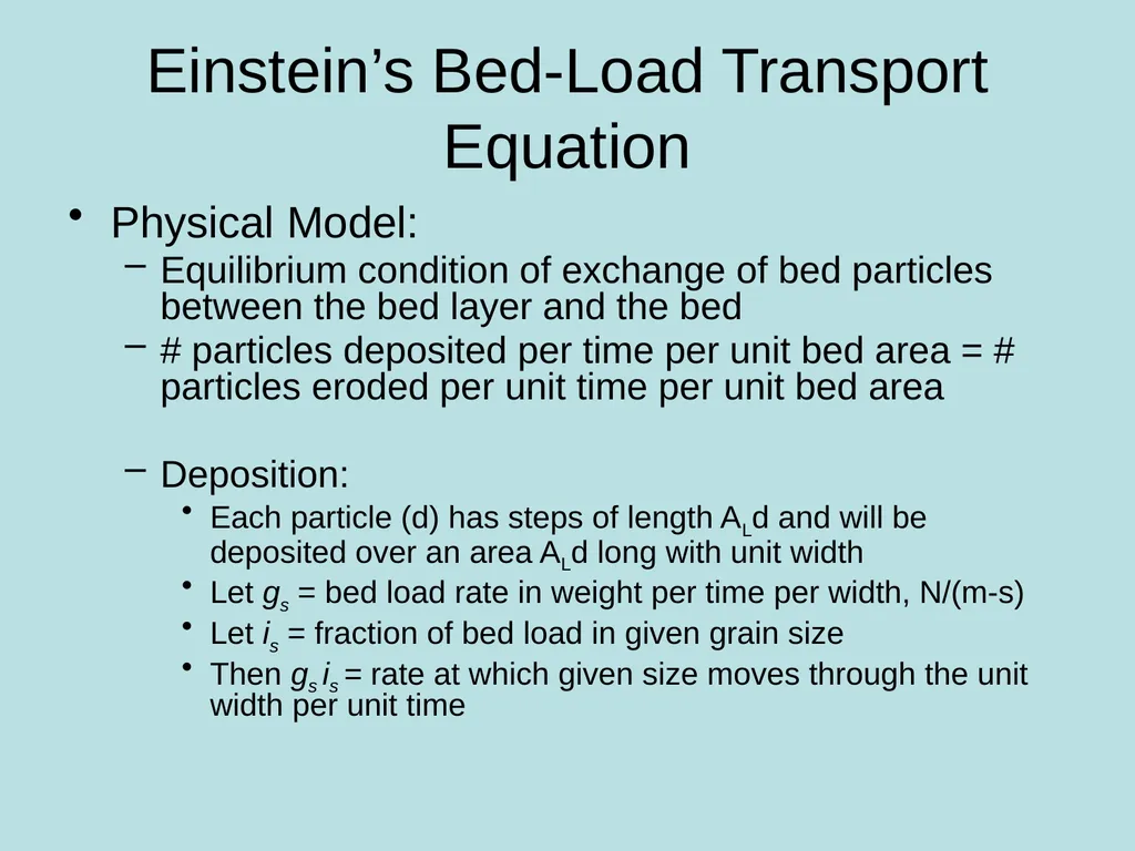
slide43. Einstein’s Bed-Load Transport Equation Physical Model:
Equilibrium condition of exchange of bed particles between the bed layer and the bed
# particles deposited per time per unit bed area = # particles eroded per unit time per unit bed area

Deposition:
Each particle (d) has steps of length ALd and will be deposited over an area ALd long with unit width
Let gs = bed load rate in weight per time per width, N/(m-s)
Let is = fraction of bed load in given grain size
Then gs is = rate at which given size moves through the unit width per unit time<br>
slide44. Einstein’s Bed-Load Transport Equation Physical Model:
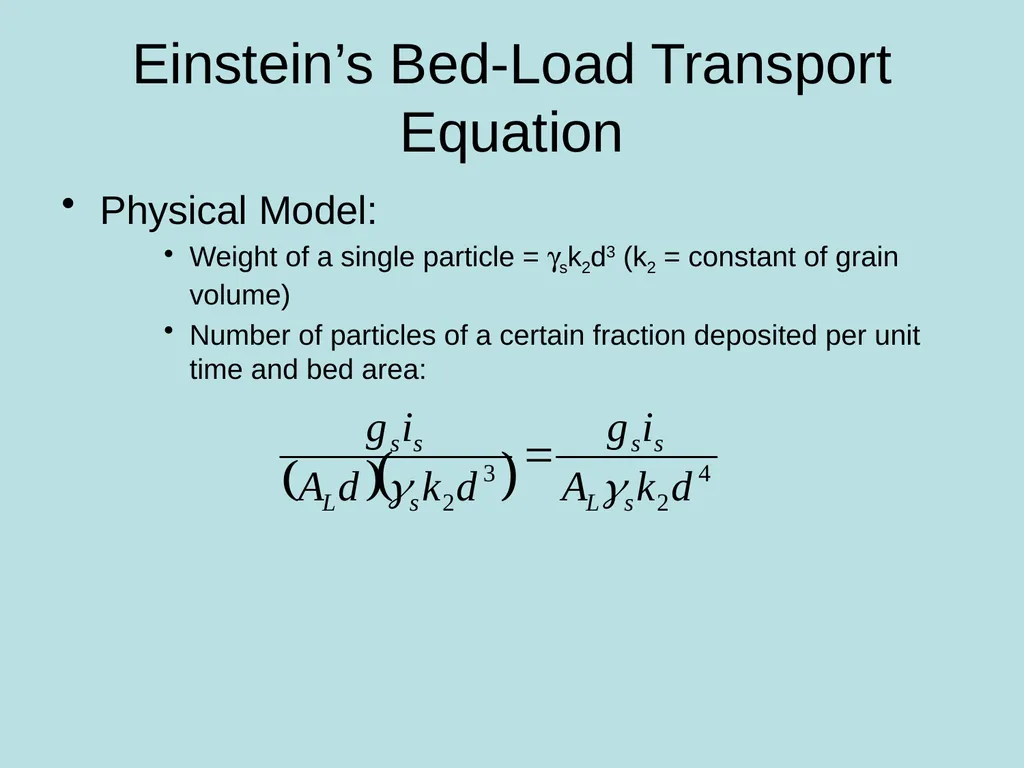
Weight of a single particle = gsk2d3 (k2 = constant of grain volume)
Number of particles of a certain fraction deposited per unit time and bed area:<br>
slide45. Einstein’s Bed-Load Transport Equation Physical Model:
Erosion:
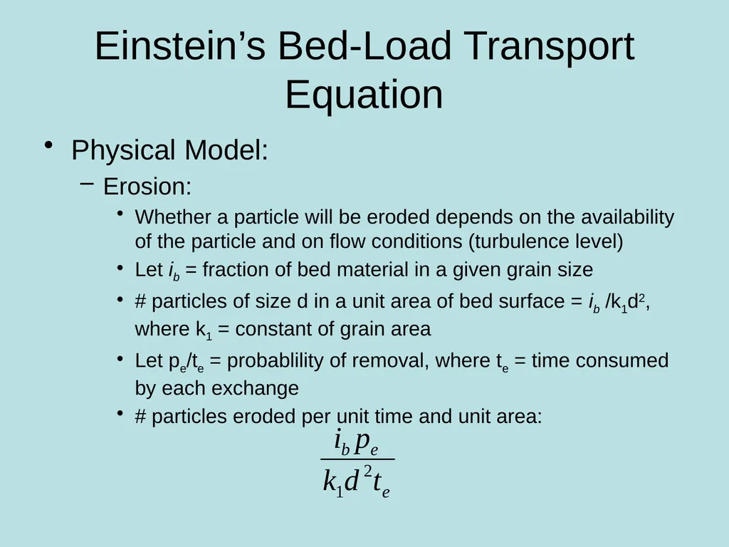
Whether a particle will be eroded depends on the availability of the particle and on flow conditions (turbulence level)
Let ib = fraction of bed material in a given grain size
# particles of size d in a unit area of bed surface = ib /k1d2, where k1 = constant of grain area
Let pe/te = probablility of removal, where te = time consumed by each exchange
# particles eroded per unit time and unit area:<br>
slide46. Einstein’s Bed-Load Transport Equation Physical Model:
Erosion:
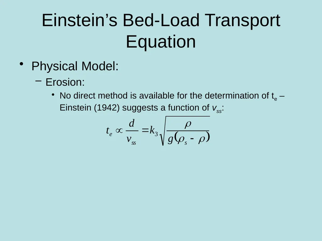
No direct method is available for the determination of te – Einstein (1942) suggests a function of vss:<br>
slide47. Einstein’s Bed-Load Transport Equation Physical Model:
Bed Load Equation (Equilibrium):
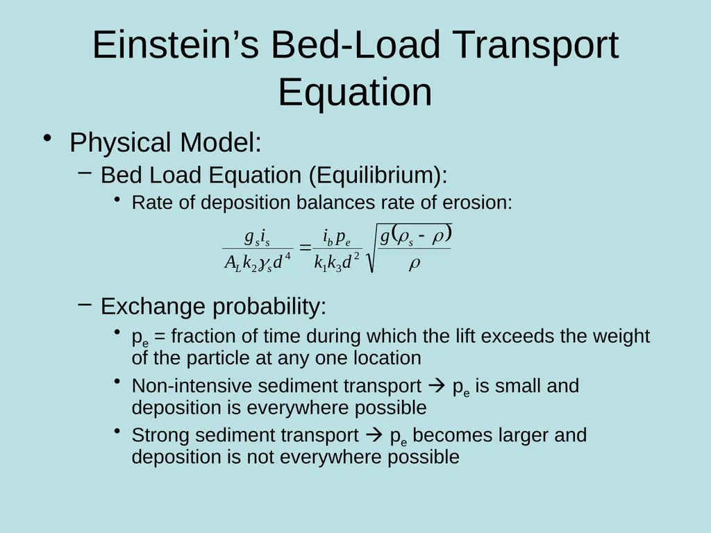
Rate of deposition balances rate of erosion:

Exchange probability:
pe = fraction of time during which the lift exceeds the weight of the particle at any one location
Non-intensive sediment transport  pe is small and deposition is everywhere possible
Strong sediment transport  pe becomes larger and deposition is not everywhere possible<br>
slide48. Einstein’s Bed-Load Transport Equation Physical Model:
Exchange probability:
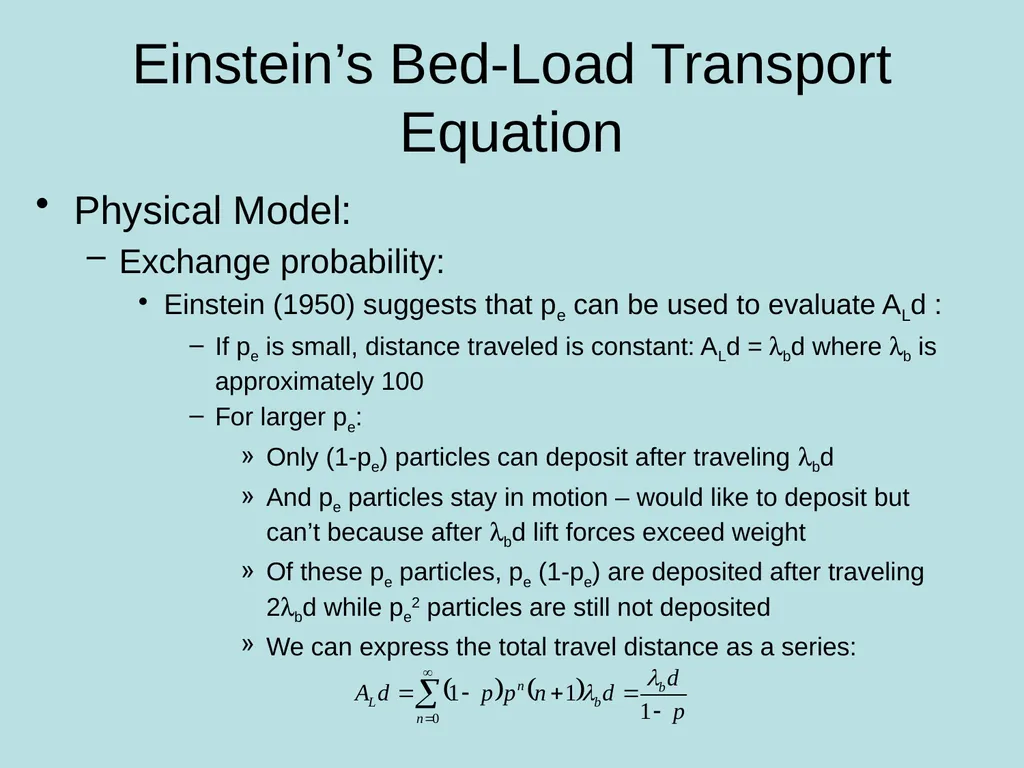
Einstein (1950) suggests that pe can be used to evaluate ALd :
If pe is small, distance traveled is constant: ALd = lbd where lb is approximately 100
For larger pe:
Only (1-pe) particles can deposit after traveling lbd
And pe particles stay in motion – would like to deposit but can’t because after lbd lift forces exceed weight
Of these pe particles, pe (1-pe) are deposited after traveling 2lbd while pe2 particles are still not deposited
We can express the total travel distance as a series:<br>
slide49. Einstein’s Bed-Load Transport Equation Physical Model:
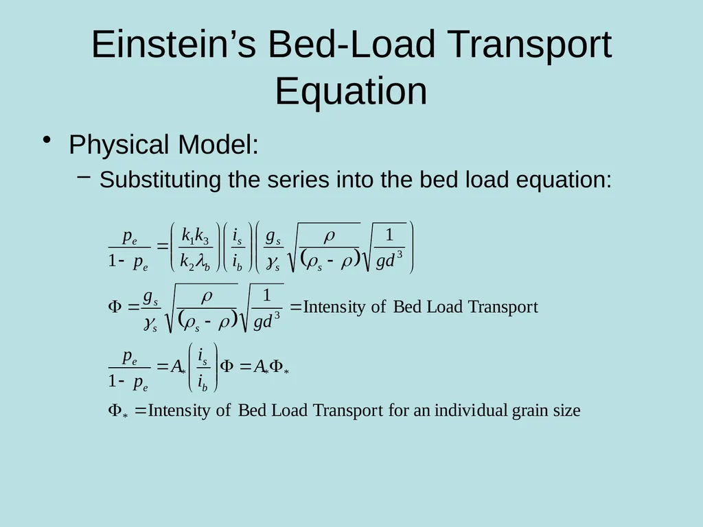
Substituting the series into the bed load equation:<br>
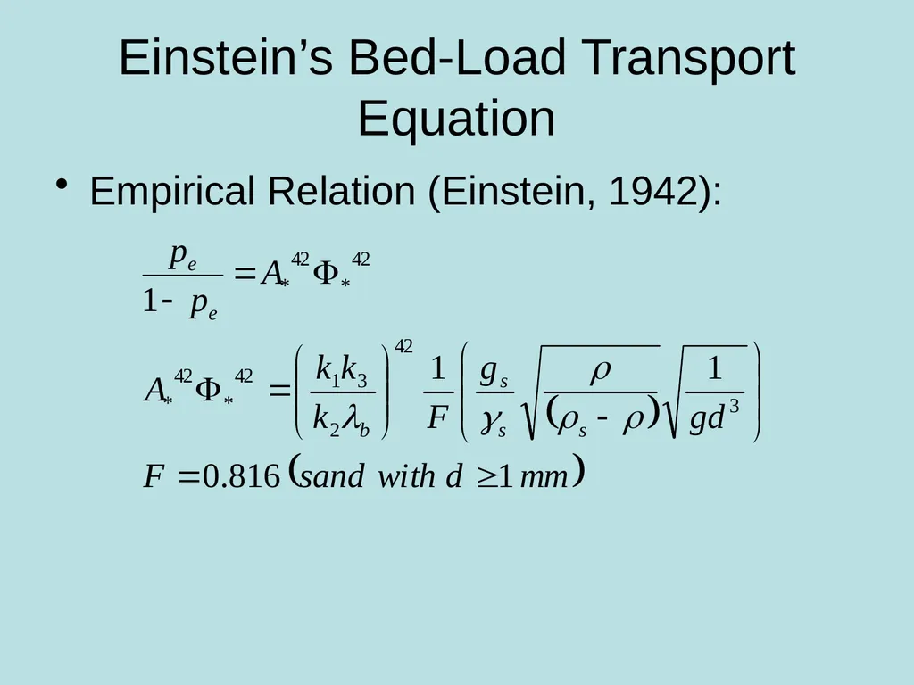
slide50. Einstein’s Bed-Load Transport Equation Empirical Relation (Einstein, 1942):<br>
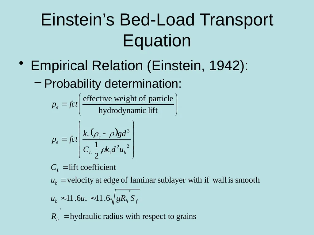
slide51. Einstein’s Bed-Load Transport Equation Empirical Relation (Einstein, 1942):
Probability determination:<br>
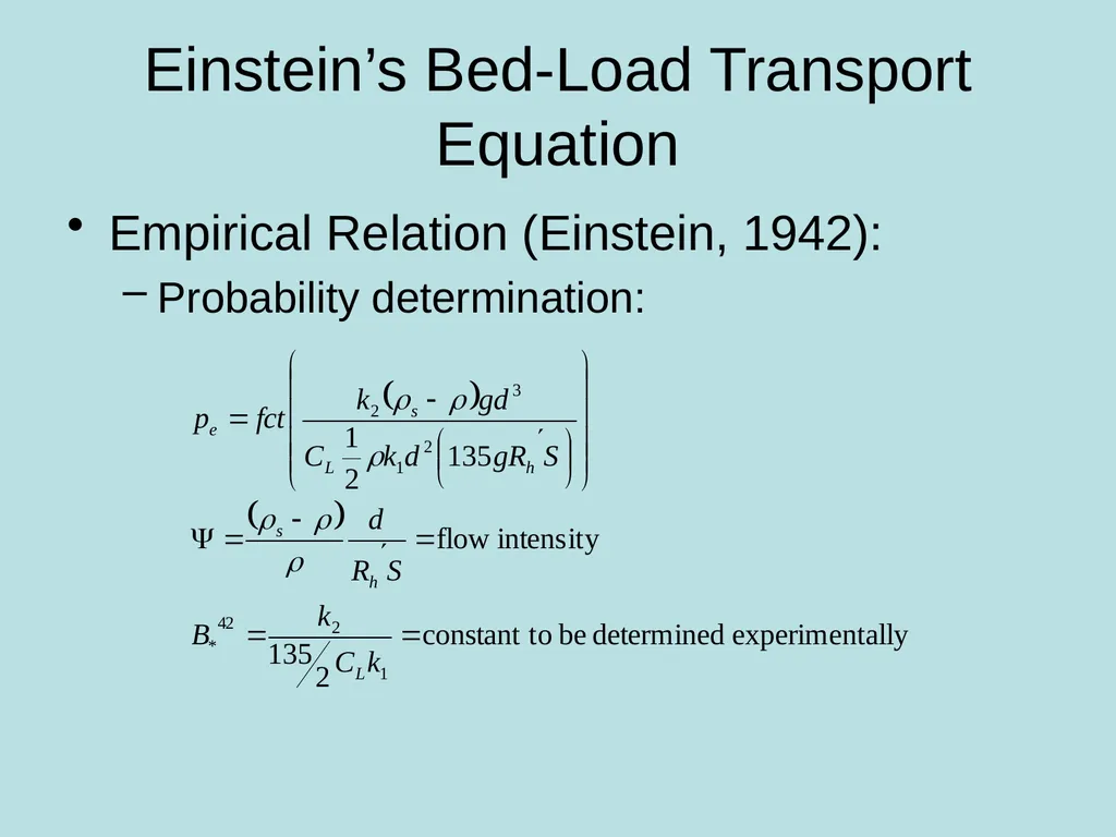
slide52. Einstein’s Bed-Load Transport Equation Empirical Relation (Einstein, 1942):
Probability determination:<br>
slide53. Einstein’s Bed-Load Transport Equation Empirical Relation (Einstein, 1942):
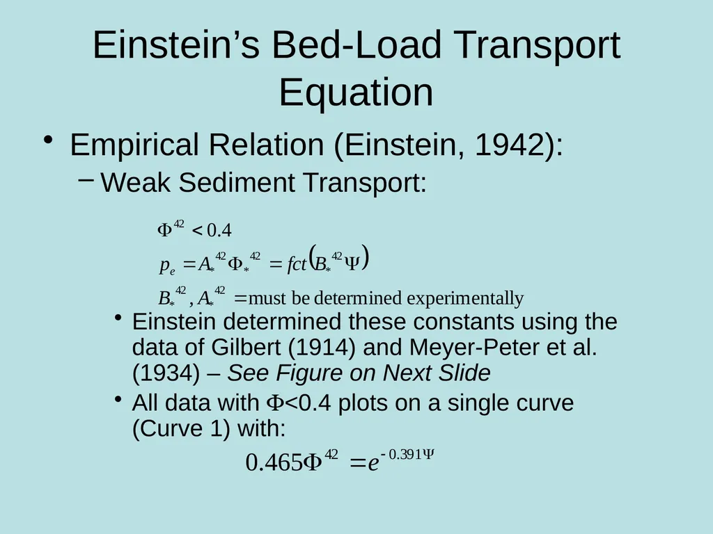
Weak Sediment Transport:

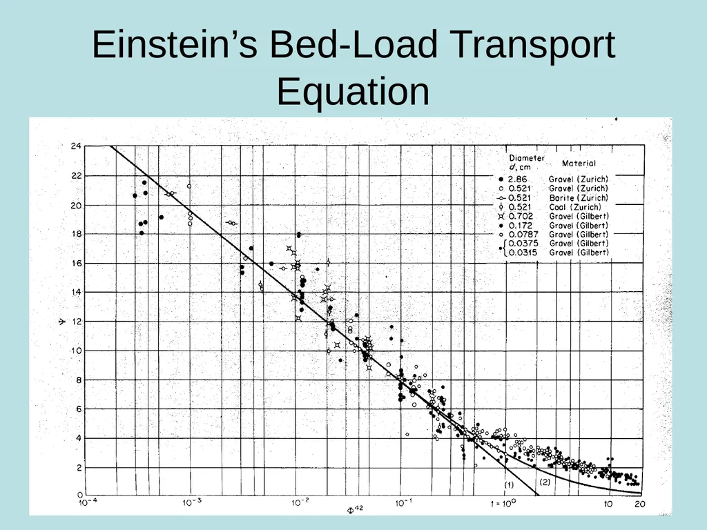
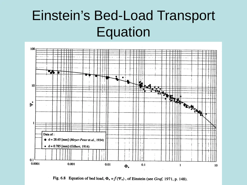
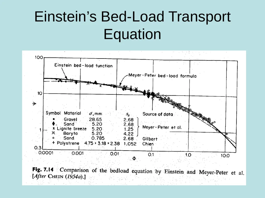
Einstein determined these constants using the data of Gilbert (1914) and Meyer-Peter et al. (1934) – See Figure on Next Slide
All data with F<0.4 plots on a single curve (Curve 1) with:<br>
slide54. Einstein’s Bed-Load Transport Equation<br>
slide55. Einstein’s Bed-Load Transport Equation Empirical Relation (Einstein, 1942):
Strong Sediment Transport:
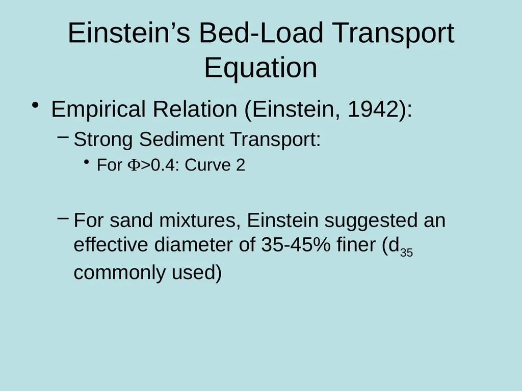
For F>0.4: Curve 2

For sand mixtures, Einstein suggested an effective diameter of 35-45% finer (d35 commonly used)<br>
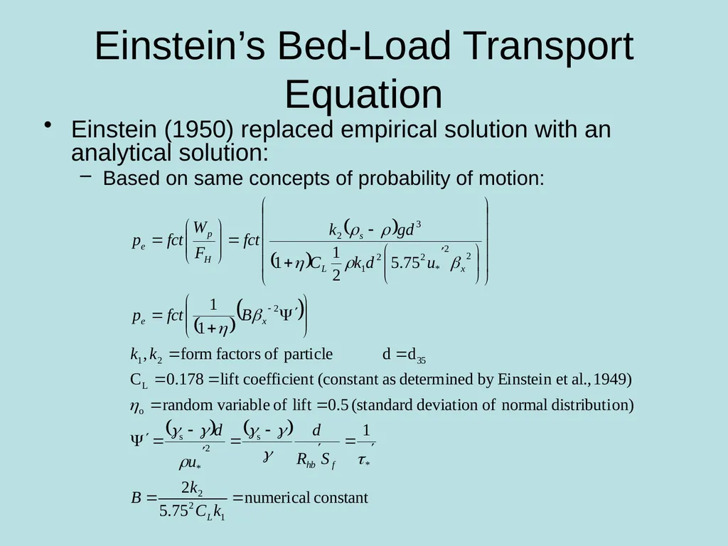
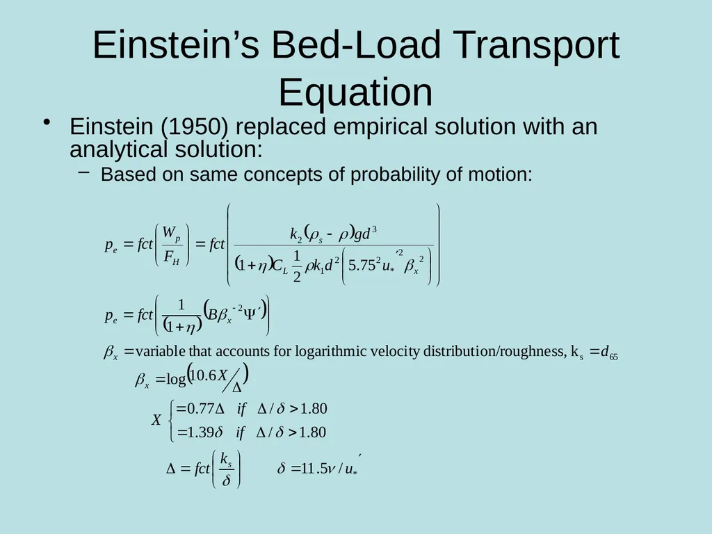
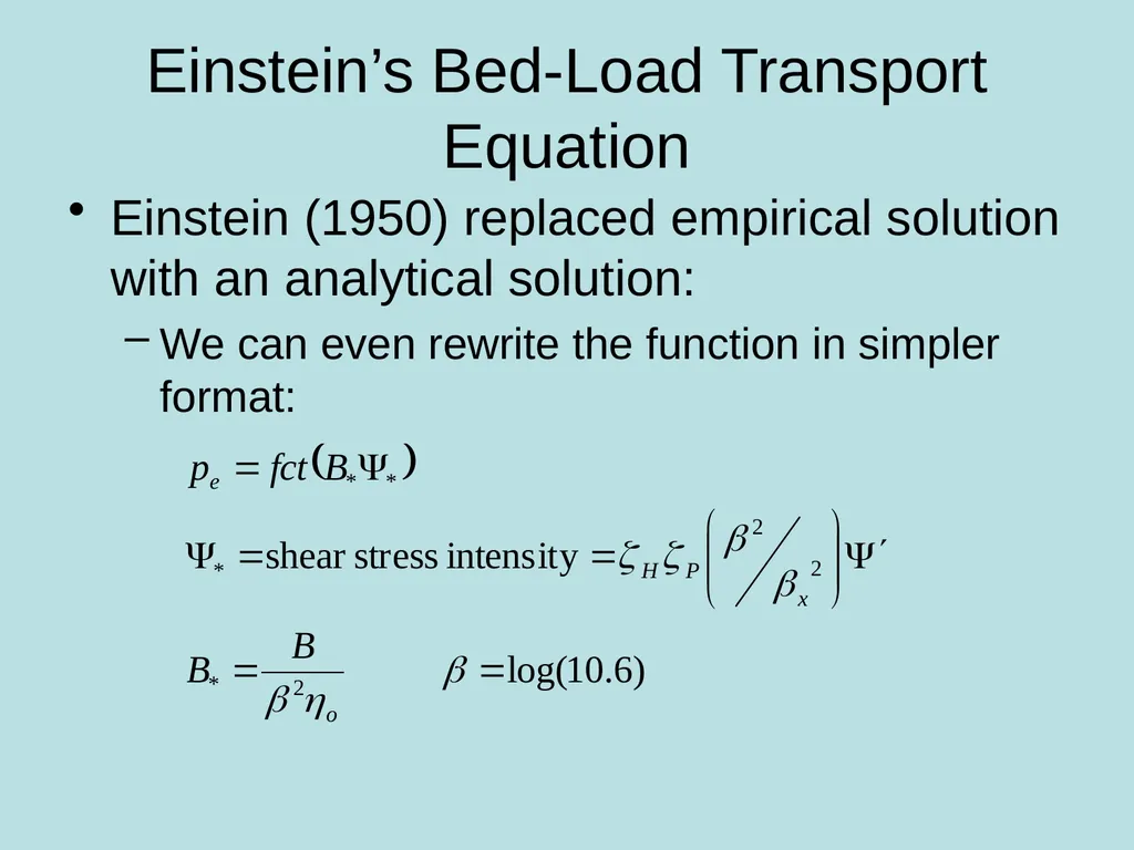
slide56. Einstein’s Bed-Load Transport Equation Einstein (1950) replaced empirical solution with an analytical solution:
Based on same concepts of probability of motion:<br>
slide57. Einstein’s Bed-Load Transport Equation Einstein (1950) replaced empirical solution with an analytical solution:
Based on same concepts of probability of motion:<br>
slide58. Einstein’s Bed-Load Transport Equation<br>
slide59. Einstein’s Bed-Load Transport Equation Einstein (1950) replaced empirical solution with an analytical solution:
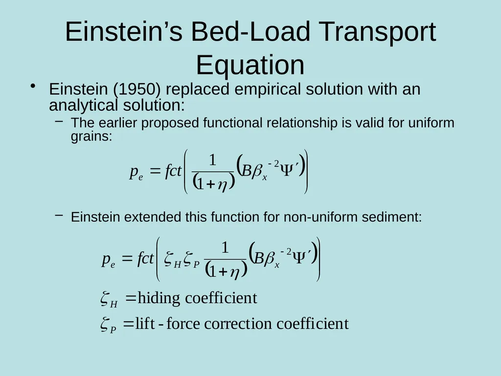
The earlier proposed functional relationship is valid for uniform grains:

Einstein extended this function for non-uniform sediment:<br>
slide60. Einstein’s Bed-Load Transport Equation<br>
slide61. Einstein’s Bed-Load Transport Equation Einstein (1950) replaced empirical solution with an analytical solution:
We can even rewrite the function in simpler format:<br>
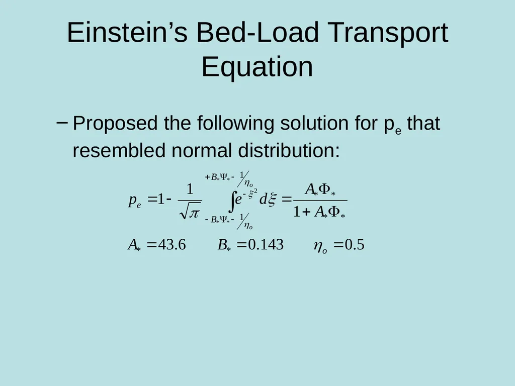
slide62. Einstein’s Bed-Load Transport Equation Proposed the following solution for pe that resembled normal distribution:<br>
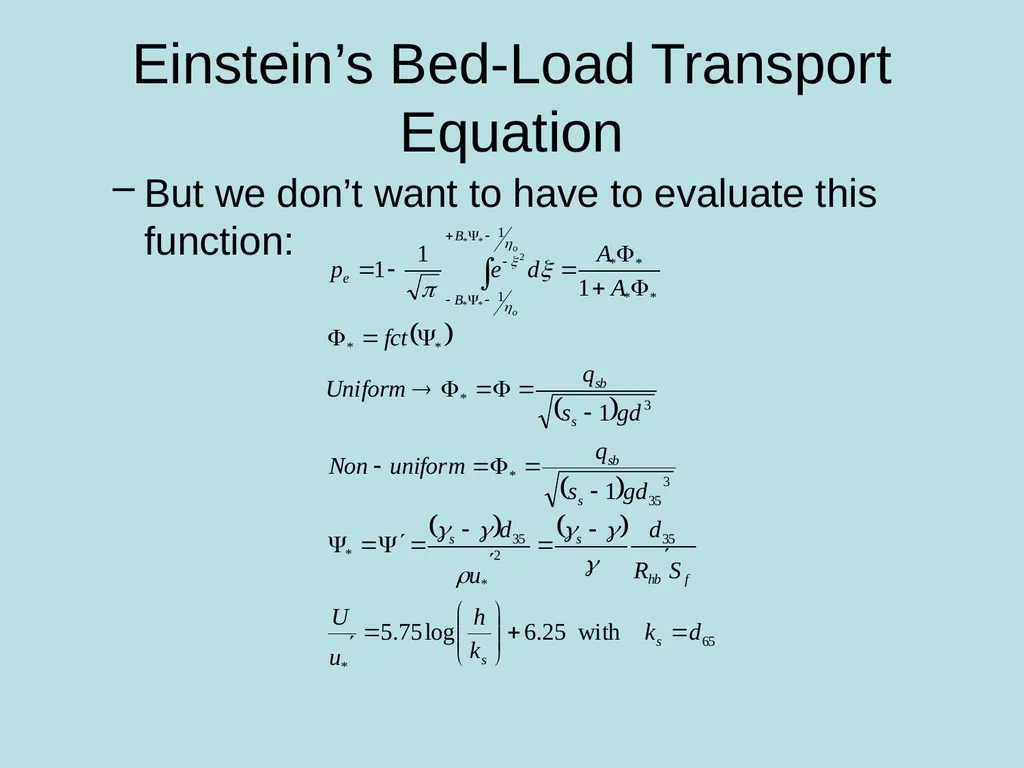
slide63. Einstein’s Bed-Load Transport Equation But we don’t want to have to evaluate this function:<br>
slide64. Einstein’s Bed-Load Transport Equation<br>
slide65. Einstein’s Bed-Load Transport Equation<br>
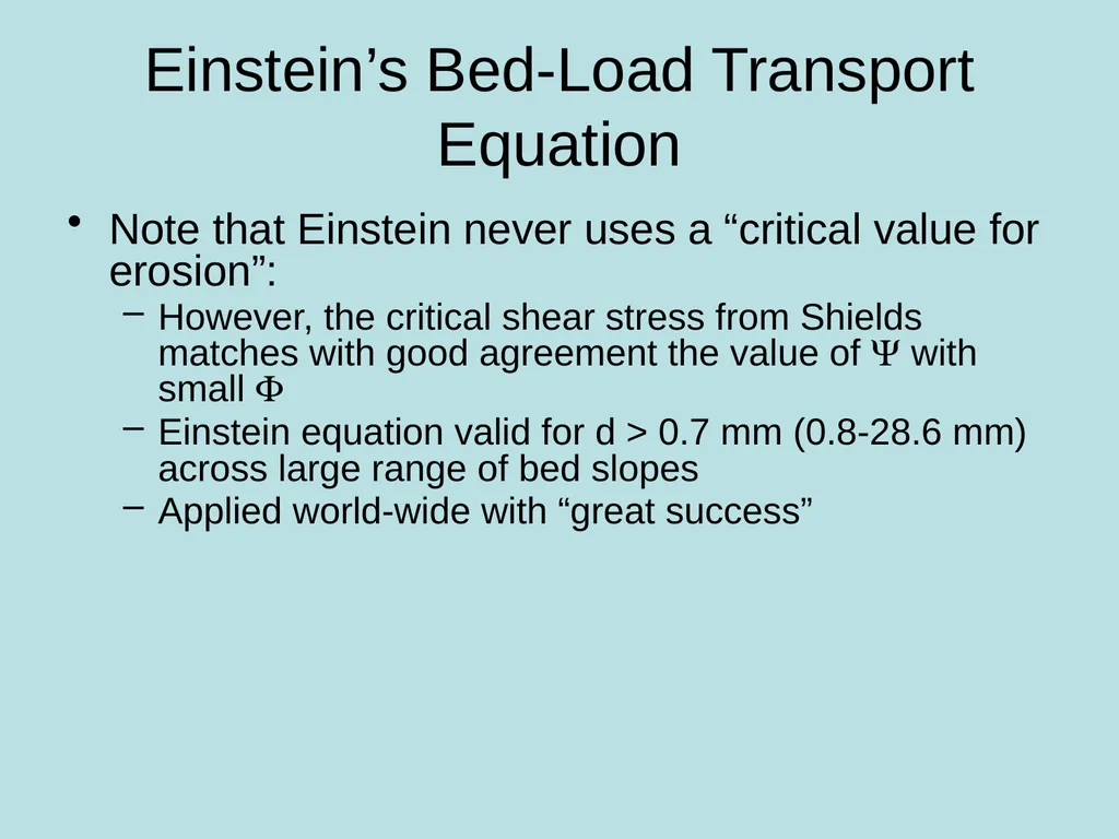
slide66. Einstein’s Bed-Load Transport Equation Note that Einstein never uses a “critical value for erosion”:
However, the critical shear stress from Shields matches with good agreement the value of Y with small F
Einstein equation valid for d > 0.7 mm (0.8-28.6 mm) across large range of bed slopes
Applied world-wide with “great success”<br>
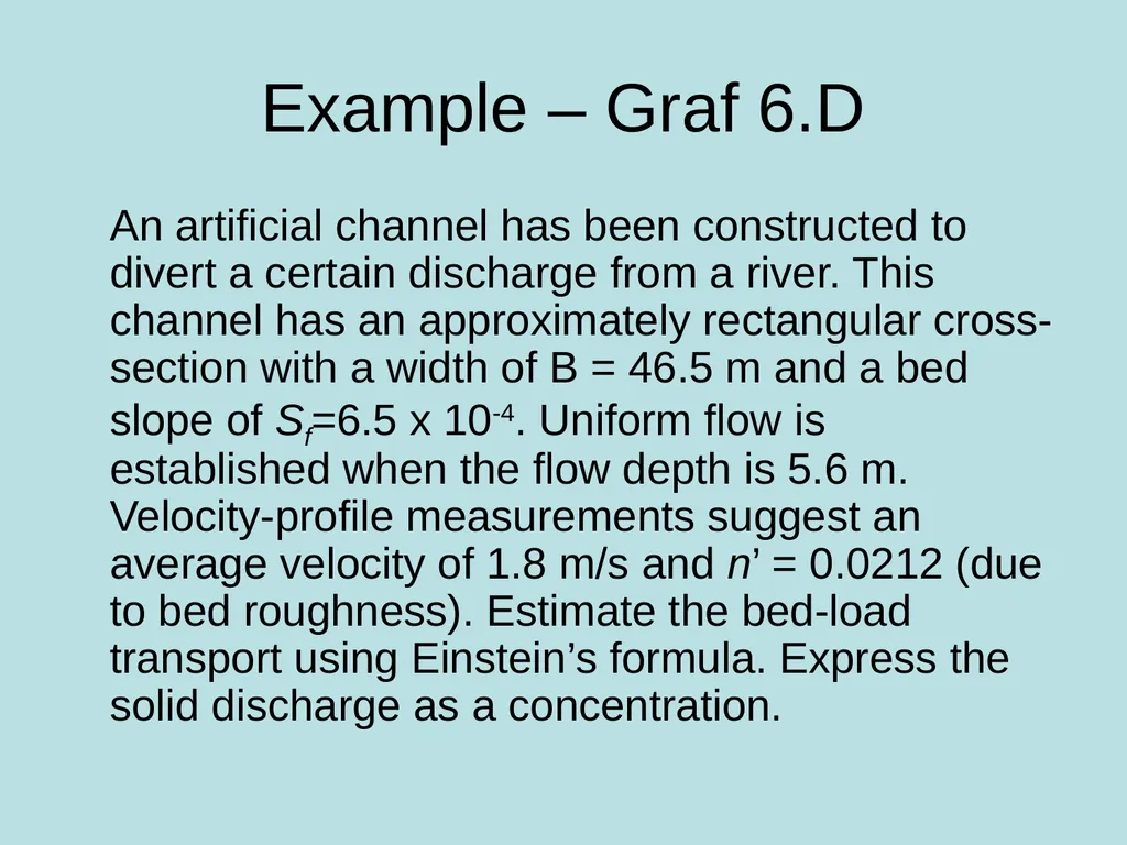
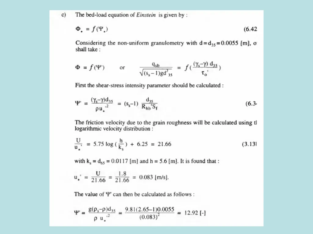
slide67. Example – Graf 6.D An artificial channel has been constructed to divert a certain discharge from a river. This channel has an approximately rectangular cross-section with a width of B = 46.5 m and a bed slope of Sf=6.5 x 10-4. Uniform flow is established when the flow depth is 5.6 m. Velocity-profile measurements suggest an average velocity of 1.8 m/s and n’ = 0.0212 (due to bed roughness). Estimate the bed-load transport using Einstein’s formula. Express the solid discharge as a concentration.<br>
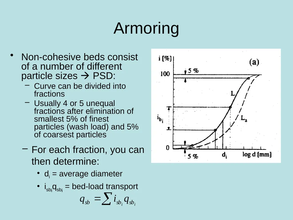
slide73. Armoring Non-cohesive beds consist of a number of different particle sizes  PSD:
Curve can be divided into fractions
Usually 4 or 5 unequal fractions after elimination of smallest 5% of finest particles (wash load) and 5% of coarsest particles For each fraction, you can then determine:
di = average diameter
isbiqsbi = bed-load transport<br>
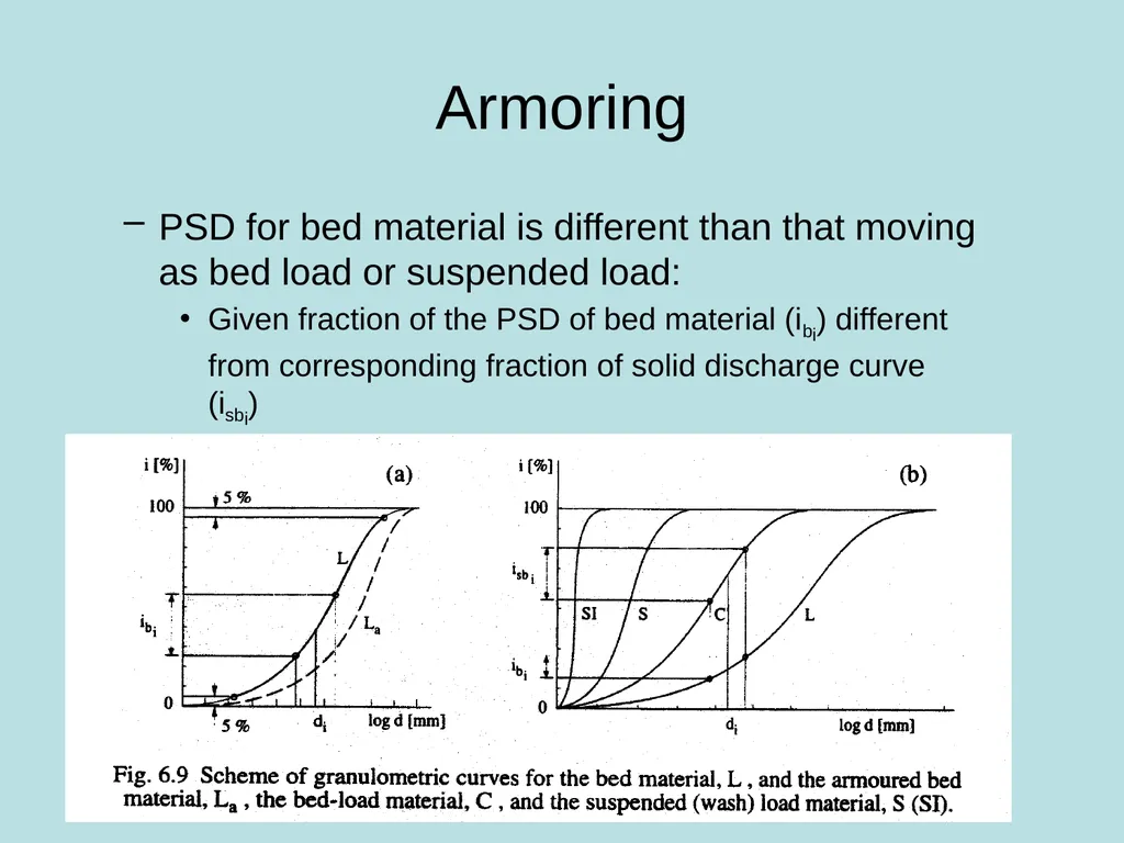
slide74. Armoring PSD for bed material is different than that moving as bed load or suspended load:
Given fraction of the PSD of bed material (ibi) different from corresponding fraction of solid discharge curve (isbi)<br>
slide75. Armoring Smaller particles are more easily eroded than larger ones:
Grain-size sorting process
Accumulation of the remaining larger particles called armoring (armouring) – protects the underlying sediment
Prevents erosion during subsequent flood events due to larger particles at bed surface
Capacity for sediment transport not satisfied until armor layer is destroyed (original sediment reappears and begins to form a new armor layer)
Samples taken when armoring has occurred must be interpreted with caution!
Less than a single complete covering layer suffices for total armoring effect
Field observations suggest that a relatively stable armor layer requires a minimum of two layers of armoring particles

Question: At what location in the channel cross-section would armoring begin?<br>
slide76. Armoring Graf describes armoring as an asymptotic process:
As u* increases, smaller particles are eroded and larges ones stay in place
Corresponding friction velocity once larger ones stay in place = critical friction velocity for armoring (u*a,cr)
Maximum possible armored bed formed by largest particles: d90 or larger
For discharges when u>u*a,cr, armored bed becomes unstable and will be destroyed
Original sediment sizes will be exposed at surface and active erosion begins again
Armor can then be restored under moderate flows<br>
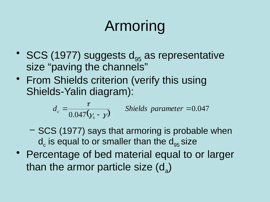
slide77. Armoring SCS (1977) suggests d95 as representative size “paving the channels”
From Shields criterion (verify this using Shields-Yalin diagram):

SCS (1977) says that armoring is probable when dc is equal to or smaller than the d95 size
Percentage of bed material equal to or larger than the armor particle size (da)<br>
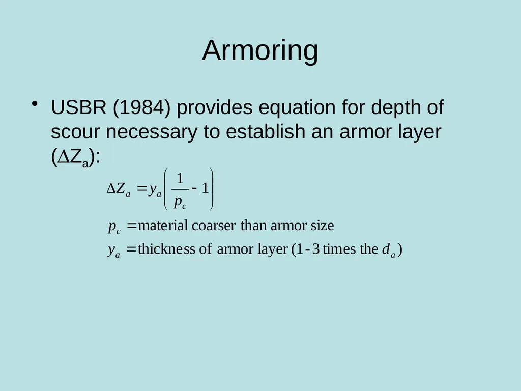
slide78. Armoring USBR (1984) provides equation for depth of scour necessary to establish an armor layer (DZa):<br>
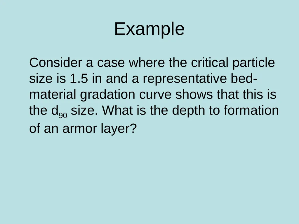
slide79. Example Consider a case where the critical particle size is 1.5 in and a representative bed-material gradation curve shows that this is the d90 size. What is the depth to formation of an armor layer?<br>
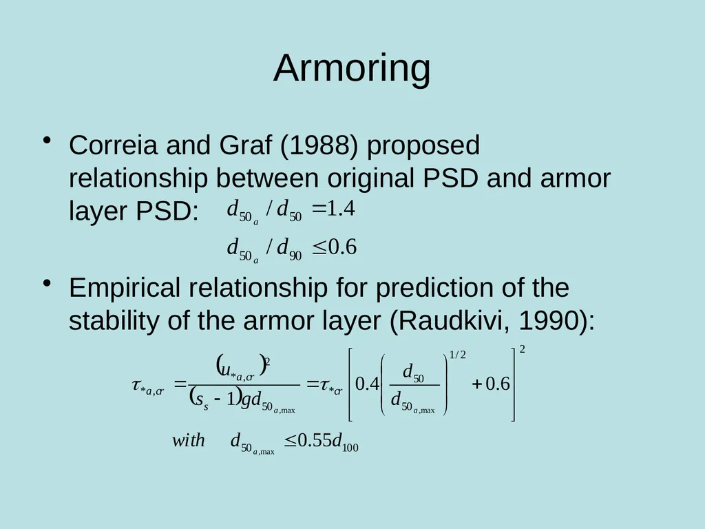
slide80. Armoring Correia and Graf (1988) proposed relationship between original PSD and armor layer PSD:

Empirical relationship for prediction of the stability of the armor layer (Raudkivi, 1990):<br>
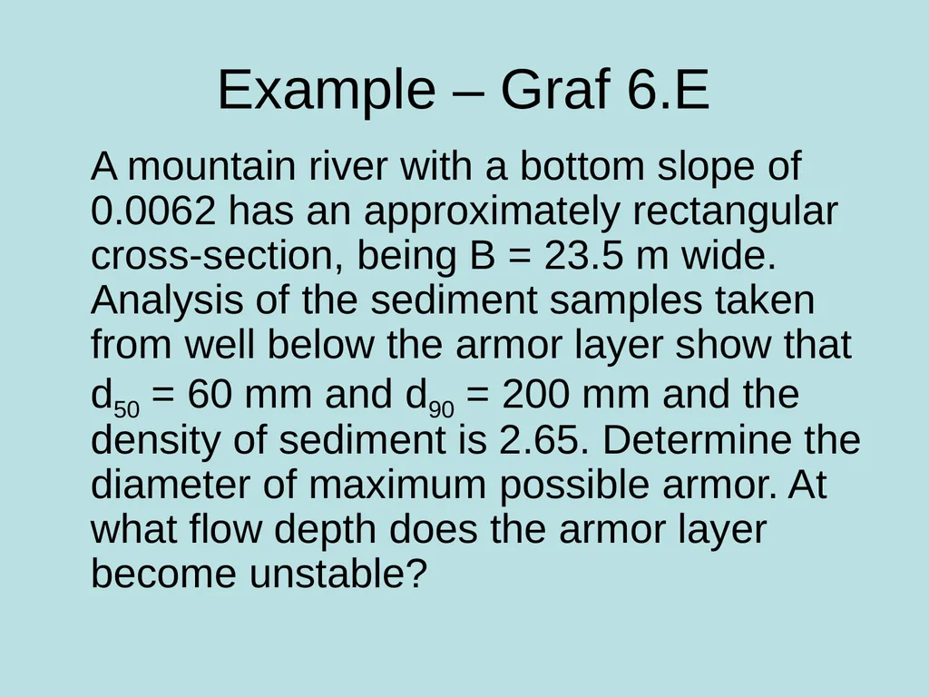
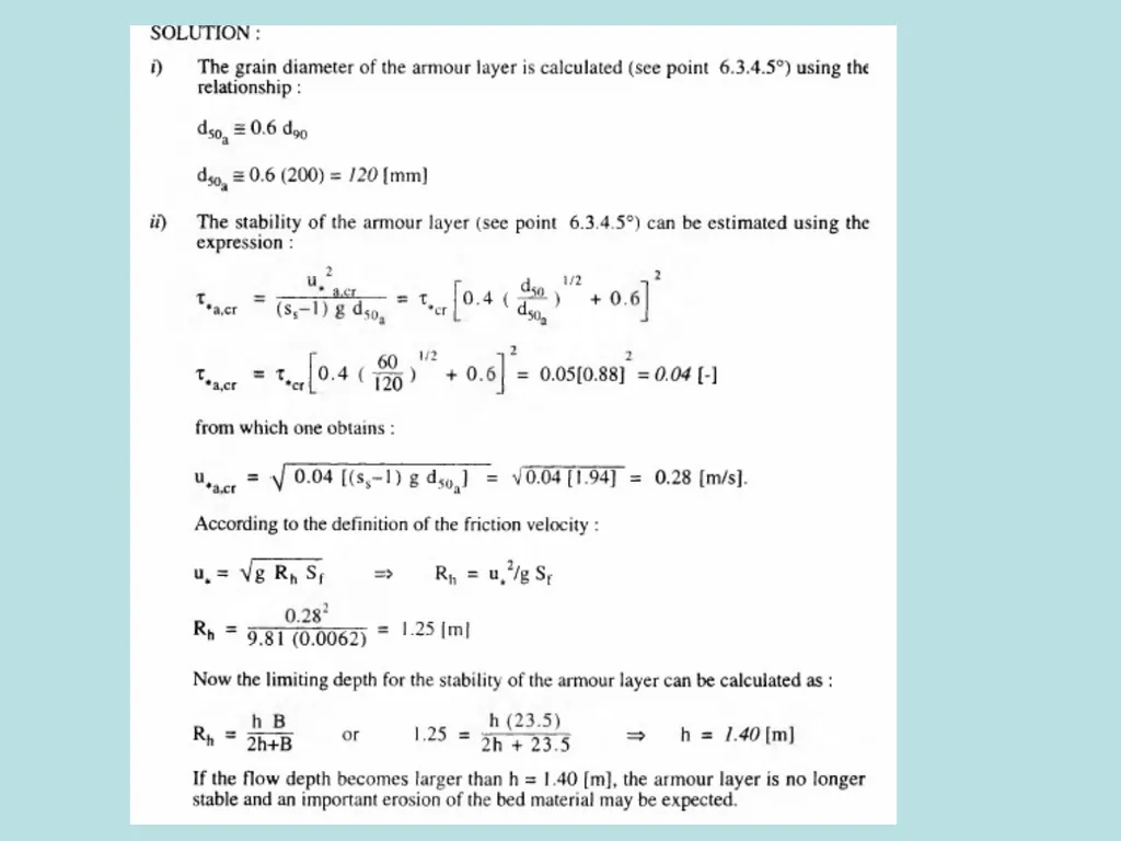
slide81. Example – Graf 6.E A mountain river with a bottom slope of 0.0062 has an approximately rectangular cross-section, being B = 23.5 m wide. Analysis of the sediment samples taken from well below the armor layer show that d50 = 60 mm and d90 = 200 mm and the density of sediment is 2.65. Determine the diameter of maximum possible armor. At what flow depth does the armor layer become unstable?<br>