
Google Earth Engine Introduction 1 Outline What is
A
Published · 69 slides · 0 views
1 / 1



Description
Google Earth Engine Introduction 1 Outline What is GEE? Practical to get you started introduce some functionality to GEE API Advanced practical on queries Use satellite data and shapefiles to query something Extra bonus At end is a run
Related Topics
Share
Embed code
Download this presentation From Below
"Google Earth Engine Introduction 1 Outline What is" is the property of its rightful owner. Permission is granted to download and print the materials on this website for personal, non-commercial use only, and to display it on your personal computer provided you do not modify the materials and that you retain all copyright notices contained in the materials. By downloading content from our website, you accept the terms of this agreement.
Presentation Transcript
01
Google Earth Engine Introduction 1<br>
02
Outline What is GEE?
Practical to get you started
introduce some functionality to GEE API
Advanced practical on queries
Use satellite data and shapefiles to query something
Extra bonus
At end is a run through of how to get shapefiles into GEE 2<br>
Practical to get you started
introduce some functionality to GEE API
Advanced practical on queries
Use satellite data and shapefiles to query something
Extra bonus
At end is a run through of how to get shapefiles into GEE 2<br>
03
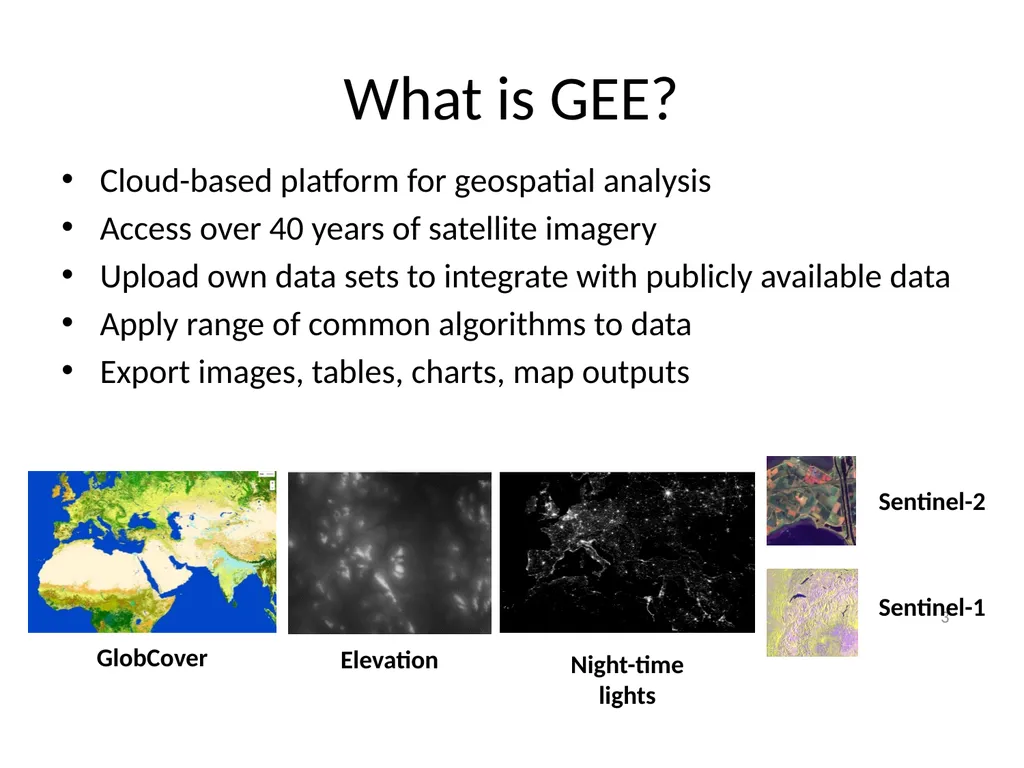
What is GEE? Cloud-based platform for geospatial analysis
Access over 40 years of satellite imagery
Upload own data sets to integrate with publicly available data
Apply range of common algorithms to data
Export images, tables, charts, map outputs 3 Elevation Sentinel-1 Sentinel-2 Night-time lights GlobCover<br>
Access over 40 years of satellite imagery
Upload own data sets to integrate with publicly available data
Apply range of common algorithms to data
Export images, tables, charts, map outputs 3 Elevation Sentinel-1 Sentinel-2 Night-time lights GlobCover<br>
04
What can you do in the API Run algorithms on image data:
Simple Band combinations such as NDVI
Masking bands using existing bands
Classifying satellite data
Subsetting data spatially using vector data
Long list of options – most would appear in ArcMap, ENVI, Erdas Imagine, R. 4<br>
Simple Band combinations such as NDVI
Masking bands using existing bands
Classifying satellite data
Subsetting data spatially using vector data
Long list of options – most would appear in ArcMap, ENVI, Erdas Imagine, R. 4<br>
05
Example: Time Series in Kenya Is it possible to estimate NDVI time series of agricultural fields in Kenya?
Method:
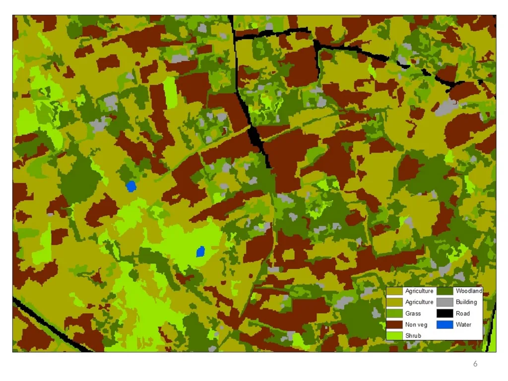
VHR Land use classification (QuickBird).
Create mask of agricultural fields
Mask landsat 5 time series from 2002-2012 to the field level. 5<br>
Method:
VHR Land use classification (QuickBird).
Create mask of agricultural fields
Mask landsat 5 time series from 2002-2012 to the field level. 5<br>
06
6<br>
07
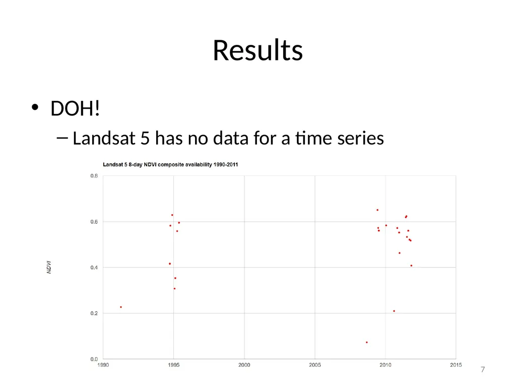
Results DOH!
Landsat 5 has no data for a time series 7<br>
Landsat 5 has no data for a time series 7<br>
08
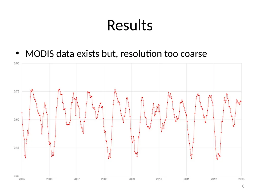
Results MODIS data exists but, resolution too coarse 8<br>
09
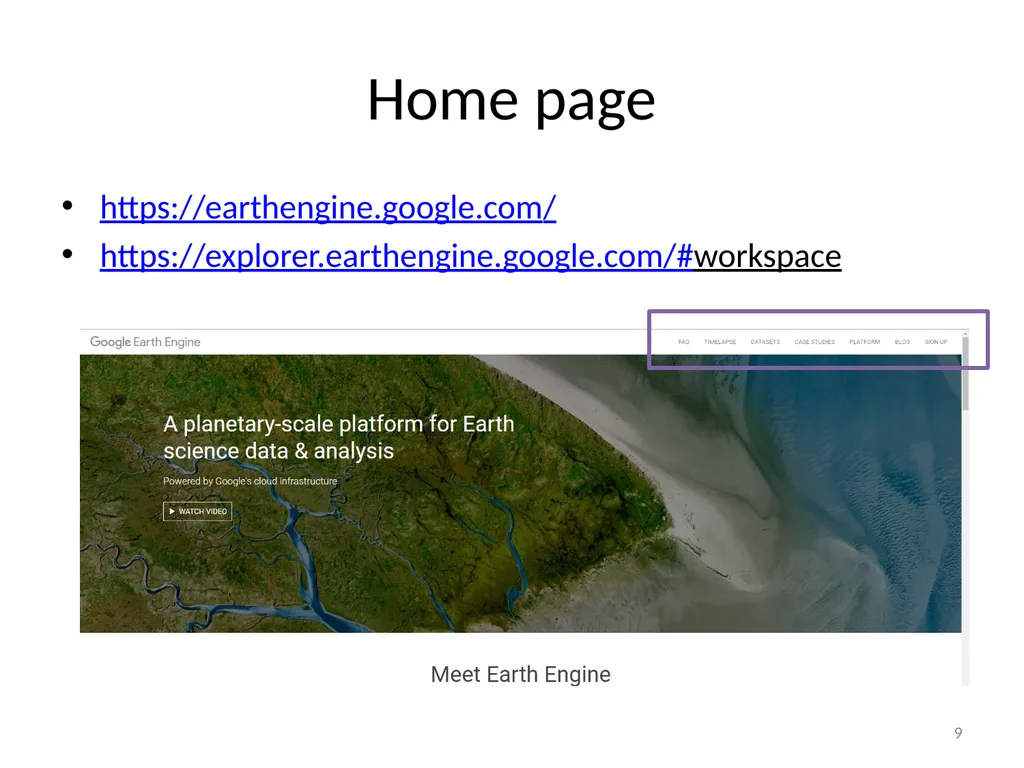
Home page https://earthengine.google.com/
https://explorer.earthengine.google.com/#workspace 9<br>
https://explorer.earthengine.google.com/#workspace 9<br>
10
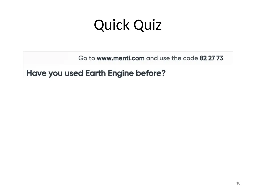
Quick Quiz 10<br>
11
11 EarthEngine API introduction<br>
12
API Introduction API requried to analyse data more fully
Mainly uses a version of JavaScript but some Python
Do not have to be a coding genius to use GEE
Many helpful tutorials:
https://developers.google.com/earth-engine/getstarted
https://developers.google.com/earth-engine/tutorials 12<br>
Mainly uses a version of JavaScript but some Python
Do not have to be a coding genius to use GEE
Many helpful tutorials:
https://developers.google.com/earth-engine/getstarted
https://developers.google.com/earth-engine/tutorials 12<br>
13
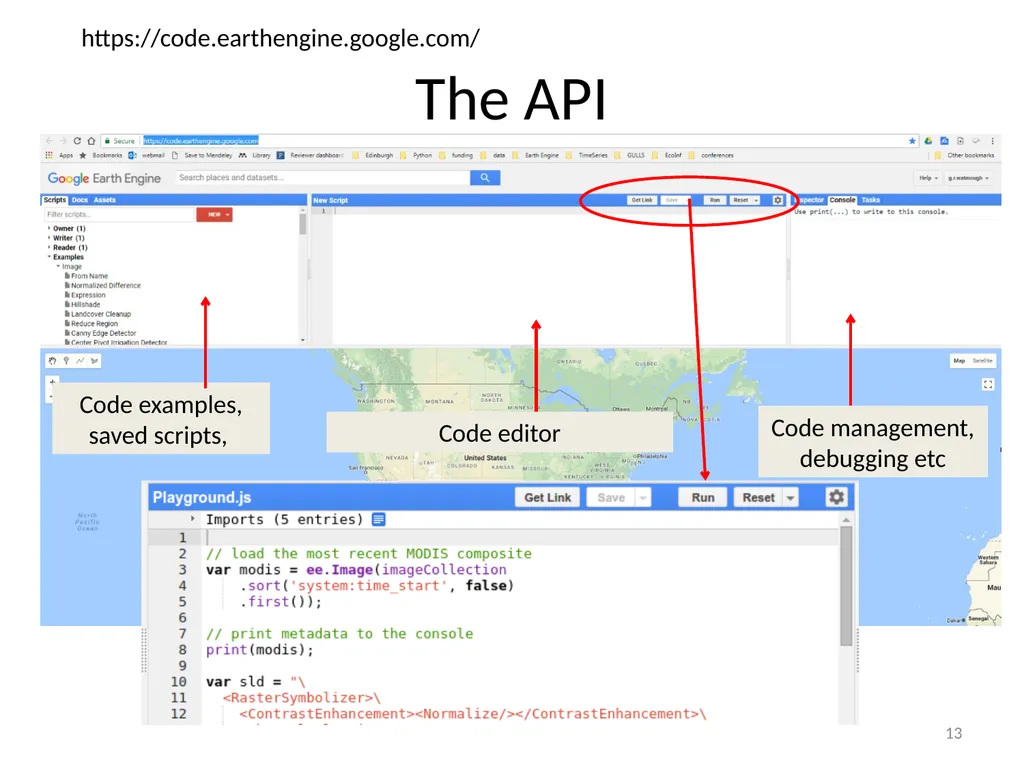
The API Code editor Code examples, saved scripts, Code management, debugging etc 13 https://code.earthengine.google.com/<br>
14
Available Algorithms Docs tab > ee.Image
Shows the algorithms that can be run on an image
Eg: Add
Click to see an explanation of the algorithm.
var image3 = image1.add(image2)
Sums the pixels in the first raster to the second raster creating a new variable (var) called image3. 14<br>
Shows the algorithms that can be run on an image
Eg: Add
Click to see an explanation of the algorithm.
var image3 = image1.add(image2)
Sums the pixels in the first raster to the second raster creating a new variable (var) called image3. 14<br>
15
15 EarthEngine API Practical 1 “Differences in NDVI"<br>
16
Before you start Have two Script windows open
Use one to paste in each new set of instructions
Once you are happy with what they are doing add them to the second script window and add a comment. Save the script for future use. 16<br>
Use one to paste in each new set of instructions
Once you are happy with what they are doing add them to the second script window and add a comment. Save the script for future use. 16<br>
17
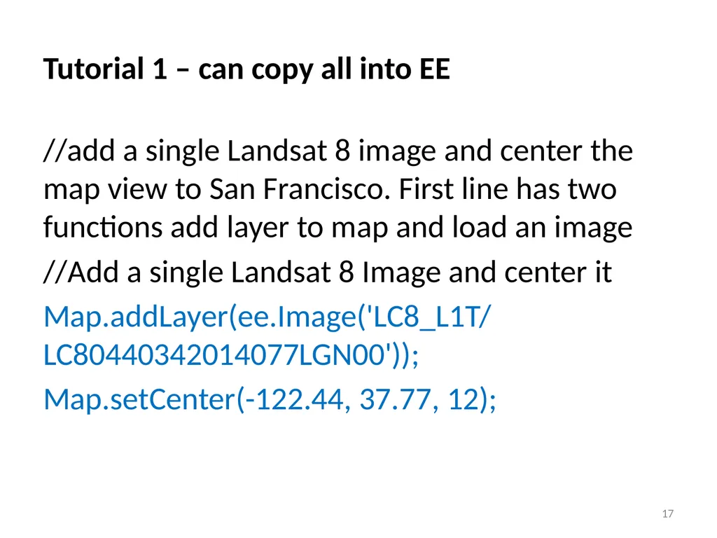
Tutorial 1 – can copy all into EE //add a single Landsat 8 image and center the map view to San Francisco. First line has two functions add layer to map and load an image
//Add a single Landsat 8 Image and center it
Map.addLayer(ee.Image('LC8_L1T/LC80440342014077LGN00'));
Map.setCenter(-122.44, 37.77, 12); 17<br>
//Add a single Landsat 8 Image and center it
Map.addLayer(ee.Image('LC8_L1T/LC80440342014077LGN00'));
Map.setCenter(-122.44, 37.77, 12); 17<br>
18
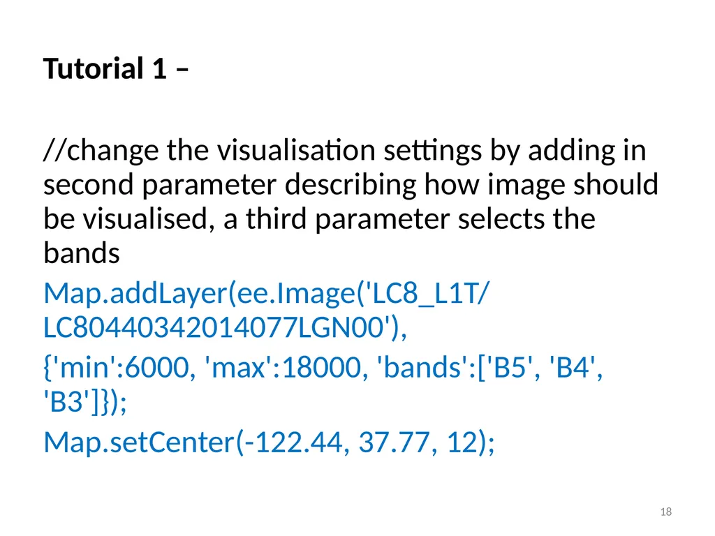
Tutorial 1 – //change the visualisation settings by adding in second parameter describing how image should be visualised, a third parameter selects the bands
Map.addLayer(ee.Image('LC8_L1T/LC80440342014077LGN00'),
{'min':6000, 'max':18000, 'bands':['B5', 'B4', 'B3']});
Map.setCenter(-122.44, 37.77, 12); 18<br>
Map.addLayer(ee.Image('LC8_L1T/LC80440342014077LGN00'),
{'min':6000, 'max':18000, 'bands':['B5', 'B4', 'B3']});
Map.setCenter(-122.44, 37.77, 12); 18<br>
19
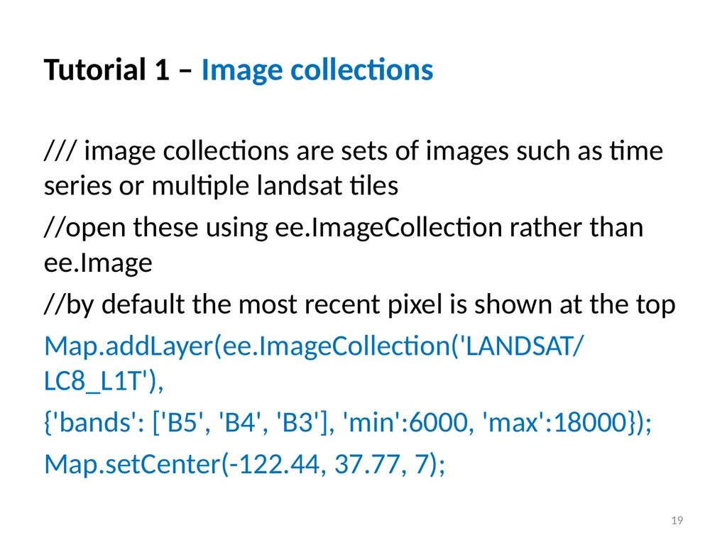
Tutorial 1 – Image collections /// image collections are sets of images such as time series or multiple landsat tiles
//open these using ee.ImageCollection rather than ee.Image
//by default the most recent pixel is shown at the top
Map.addLayer(ee.ImageCollection('LANDSAT/LC8_L1T'),
{'bands': ['B5', 'B4', 'B3'], 'min':6000, 'max':18000});
Map.setCenter(-122.44, 37.77, 7); 19<br>
//open these using ee.ImageCollection rather than ee.Image
//by default the most recent pixel is shown at the top
Map.addLayer(ee.ImageCollection('LANDSAT/LC8_L1T'),
{'bands': ['B5', 'B4', 'B3'], 'min':6000, 'max':18000});
Map.setCenter(-122.44, 37.77, 7); 19<br>
20
Tutorial 1 – improving the image view resulting image is messy due to overlapping scenes. Two ways to deal with this:
first is to select only a specific time period of images to display
second is to tell GEE how to deal with overlapping areas. 20<br>
first is to select only a specific time period of images to display
second is to tell GEE how to deal with overlapping areas. 20<br>
21
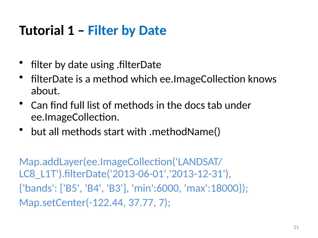
Tutorial 1 – Filter by Date filter by date using .filterDate
filterDate is a method which ee.ImageCollection knows about.
Can find full list of methods in the docs tab under ee.ImageCollection.
but all methods start with .methodName()
Map.addLayer(ee.ImageCollection('LANDSAT/LC8_L1T').filterDate('2013-06-01','2013-12-31'),
{'bands': ['B5', 'B4', 'B3'], 'min':6000, 'max':18000});
Map.setCenter(-122.44, 37.77, 7); 21<br>
filterDate is a method which ee.ImageCollection knows about.
Can find full list of methods in the docs tab under ee.ImageCollection.
but all methods start with .methodName()
Map.addLayer(ee.ImageCollection('LANDSAT/LC8_L1T').filterDate('2013-06-01','2013-12-31'),
{'bands': ['B5', 'B4', 'B3'], 'min':6000, 'max':18000});
Map.setCenter(-122.44, 37.77, 7); 21<br>
22
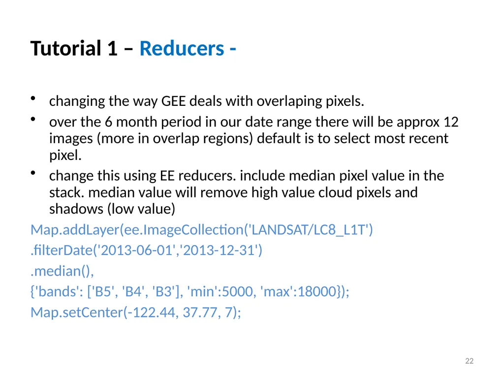
Tutorial 1 – Reducers - changing the way GEE deals with overlaping pixels.
over the 6 month period in our date range there will be approx 12 images (more in overlap regions) default is to select most recent pixel.
change this using EE reducers. include median pixel value in the stack. median value will remove high value cloud pixels and shadows (low value)
Map.addLayer(ee.ImageCollection('LANDSAT/LC8_L1T')
.filterDate('2013-06-01','2013-12-31')
.median(),
{'bands': ['B5', 'B4', 'B3'], 'min':5000, 'max':18000});
Map.setCenter(-122.44, 37.77, 7); 22<br>
over the 6 month period in our date range there will be approx 12 images (more in overlap regions) default is to select most recent pixel.
change this using EE reducers. include median pixel value in the stack. median value will remove high value cloud pixels and shadows (low value)
Map.addLayer(ee.ImageCollection('LANDSAT/LC8_L1T')
.filterDate('2013-06-01','2013-12-31')
.median(),
{'bands': ['B5', 'B4', 'B3'], 'min':5000, 'max':18000});
Map.setCenter(-122.44, 37.77, 7); 22<br>
23
Tutorial 1 – Variables The code above is getting too messy
so now use variables to hold data in
and reduce the amount of instructions in two lines
variables store values such as strings, numbers and can be called in the script
to define a variable start with var 23<br>
so now use variables to hold data in
and reduce the amount of instructions in two lines
variables store values such as strings, numbers and can be called in the script
to define a variable start with var 23<br>
24
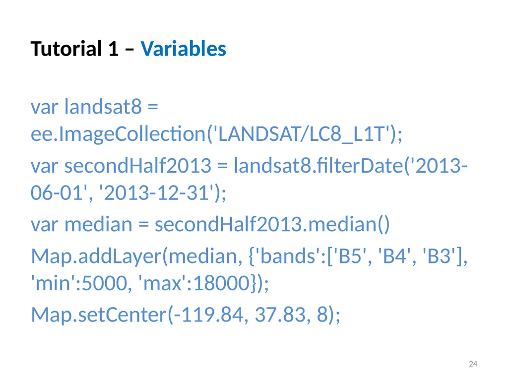
Tutorial 1 – Variables var landsat8 = ee.ImageCollection('LANDSAT/LC8_L1T');
var secondHalf2013 = landsat8.filterDate('2013-06-01', '2013-12-31');
var median = secondHalf2013.median()
Map.addLayer(median, {'bands':['B5', 'B4', 'B3'], 'min':5000, 'max':18000});
Map.setCenter(-119.84, 37.83, 8); 24<br>
var secondHalf2013 = landsat8.filterDate('2013-06-01', '2013-12-31');
var median = secondHalf2013.median()
Map.addLayer(median, {'bands':['B5', 'B4', 'B3'], 'min':5000, 'max':18000});
Map.setCenter(-119.84, 37.83, 8); 24<br>
25
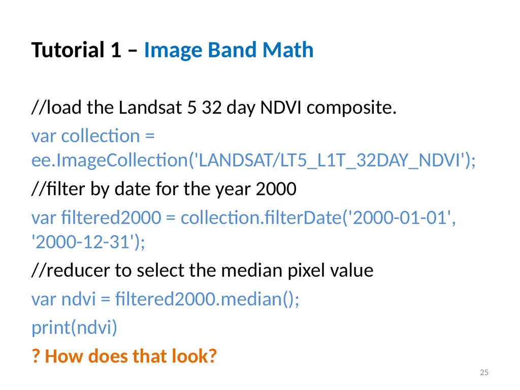
Tutorial 1 – Image Band Math //load the Landsat 5 32 day NDVI composite.
var collection = ee.ImageCollection('LANDSAT/LT5_L1T_32DAY_NDVI');
//filter by date for the year 2000
var filtered2000 = collection.filterDate('2000-01-01', '2000-12-31');
//reducer to select the median pixel value
var ndvi = filtered2000.median();
print(ndvi)
? How does that look? 25<br>
var collection = ee.ImageCollection('LANDSAT/LT5_L1T_32DAY_NDVI');
//filter by date for the year 2000
var filtered2000 = collection.filterDate('2000-01-01', '2000-12-31');
//reducer to select the median pixel value
var ndvi = filtered2000.median();
print(ndvi)
? How does that look? 25<br>
26
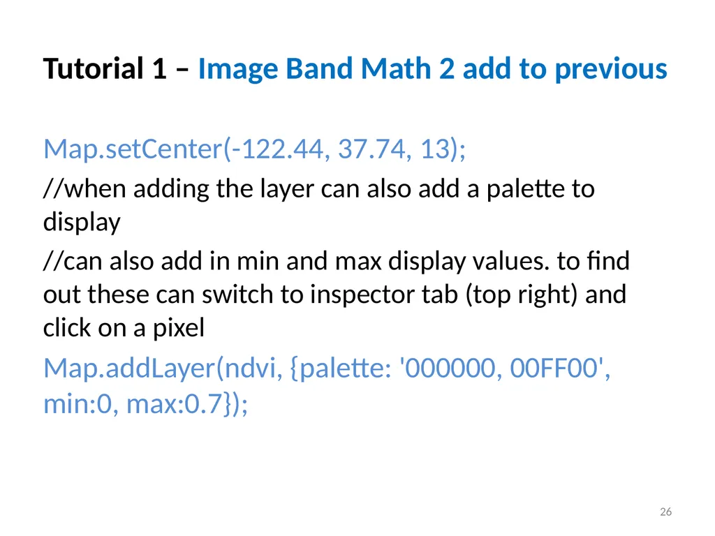
Tutorial 1 – Image Band Math 2 add to previous Map.setCenter(-122.44, 37.74, 13);
//when adding the layer can also add a palette to display
//can also add in min and max display values. to find out these can switch to inspector tab (top right) and click on a pixel
Map.addLayer(ndvi, {palette: '000000, 00FF00', min:0, max:0.7}); 26<br>
//when adding the layer can also add a palette to display
//can also add in min and max display values. to find out these can switch to inspector tab (top right) and click on a pixel
Map.addLayer(ndvi, {palette: '000000, 00FF00', min:0, max:0.7}); 26<br>
27
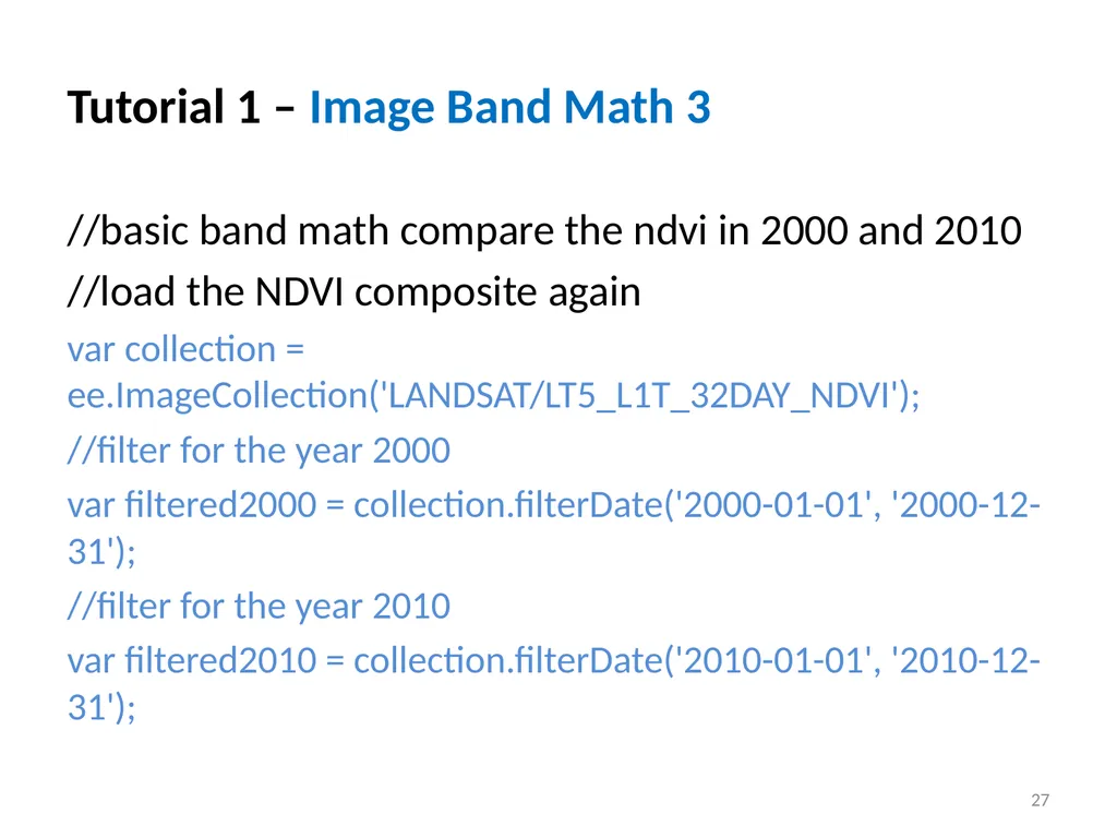
Tutorial 1 – Image Band Math 3 //basic band math compare the ndvi in 2000 and 2010
//load the NDVI composite again
var collection = ee.ImageCollection('LANDSAT/LT5_L1T_32DAY_NDVI');
//filter for the year 2000
var filtered2000 = collection.filterDate('2000-01-01', '2000-12-31');
//filter for the year 2010
var filtered2010 = collection.filterDate('2010-01-01', '2010-12-31'); 27<br>
//load the NDVI composite again
var collection = ee.ImageCollection('LANDSAT/LT5_L1T_32DAY_NDVI');
//filter for the year 2000
var filtered2000 = collection.filterDate('2000-01-01', '2000-12-31');
//filter for the year 2010
var filtered2010 = collection.filterDate('2010-01-01', '2010-12-31'); 27<br>
28
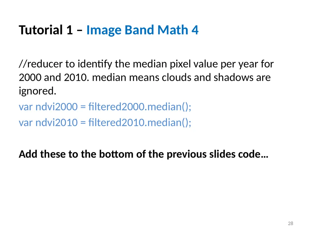
Tutorial 1 – Image Band Math 4 //reducer to identify the median pixel value per year for 2000 and 2010. median means clouds and shadows are ignored.
var ndvi2000 = filtered2000.median();
var ndvi2010 = filtered2010.median();
Add these to the bottom of the previous slides code… 28<br>
var ndvi2000 = filtered2000.median();
var ndvi2010 = filtered2010.median();
Add these to the bottom of the previous slides code… 28<br>
29
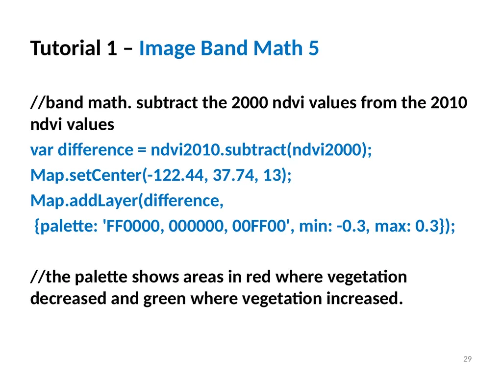
Tutorial 1 – Image Band Math 5 //band math. subtract the 2000 ndvi values from the 2010 ndvi values
var difference = ndvi2010.subtract(ndvi2000);
Map.setCenter(-122.44, 37.74, 13);
Map.addLayer(difference,
{palette: 'FF0000, 000000, 00FF00', min: -0.3, max: 0.3});
//the palette shows areas in red where vegetation decreased and green where vegetation increased. 29<br>
var difference = ndvi2010.subtract(ndvi2000);
Map.setCenter(-122.44, 37.74, 13);
Map.addLayer(difference,
{palette: 'FF0000, 000000, 00FF00', min: -0.3, max: 0.3});
//the palette shows areas in red where vegetation decreased and green where vegetation increased. 29<br>
30
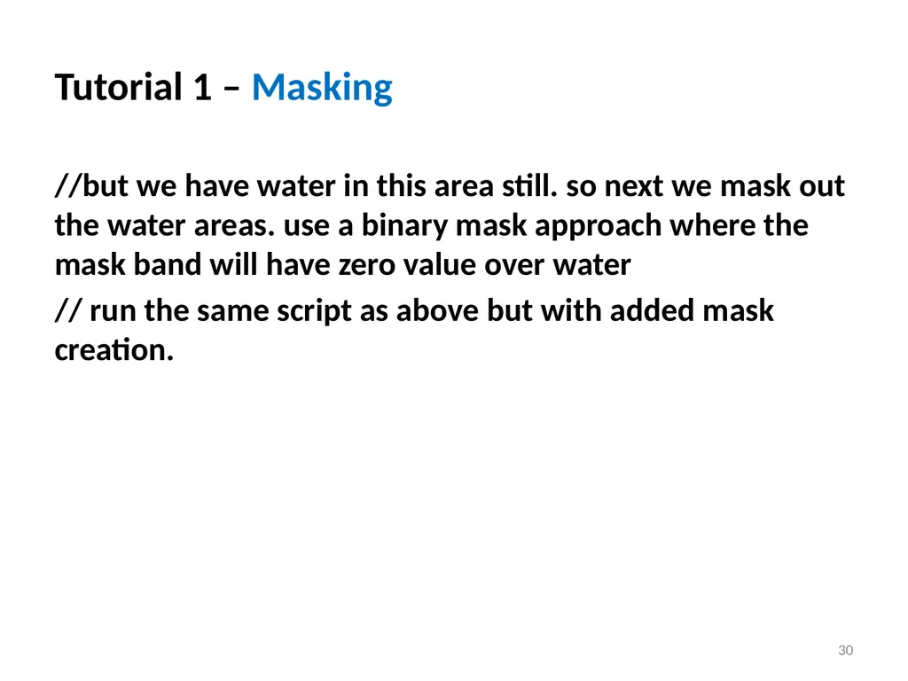
Tutorial 1 – Masking //but we have water in this area still. so next we mask out the water areas. use a binary mask approach where the mask band will have zero value over water
// run the same script as above but with added mask creation. 30<br>
// run the same script as above but with added mask creation. 30<br>
31
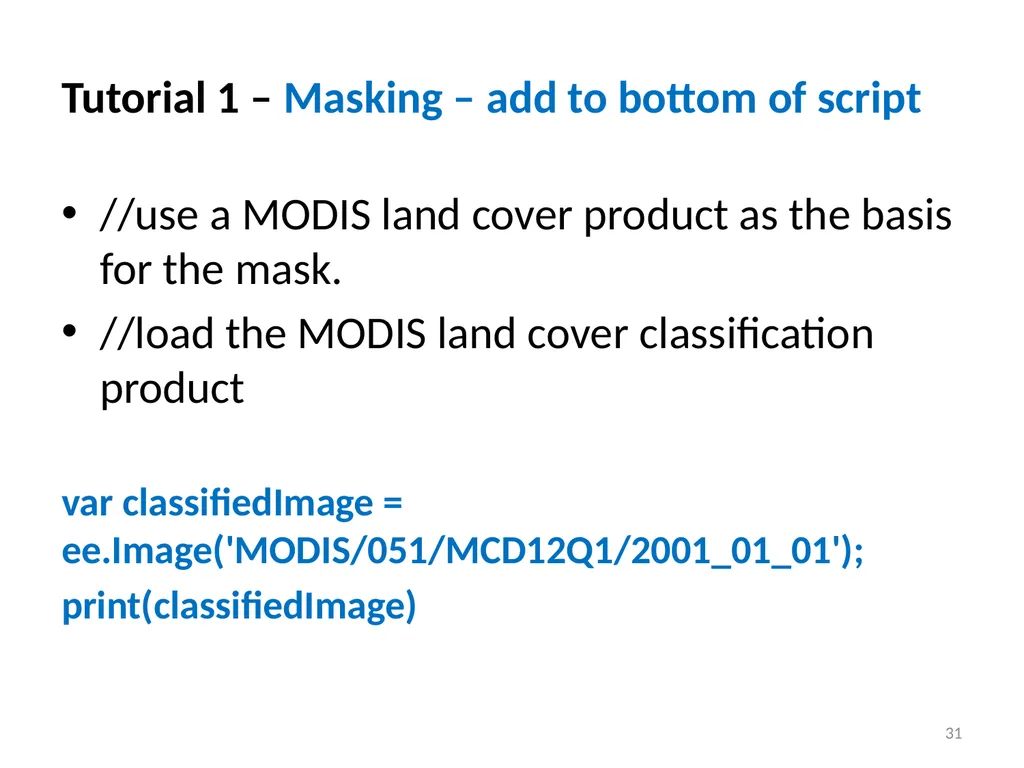
Tutorial 1 – Masking – add to bottom of script //use a MODIS land cover product as the basis for the mask.
//load the MODIS land cover classification product
var classifiedImage = ee.Image('MODIS/051/MCD12Q1/2001_01_01');
print(classifiedImage) 31<br>
//load the MODIS land cover classification product
var classifiedImage = ee.Image('MODIS/051/MCD12Q1/2001_01_01');
print(classifiedImage) 31<br>
32
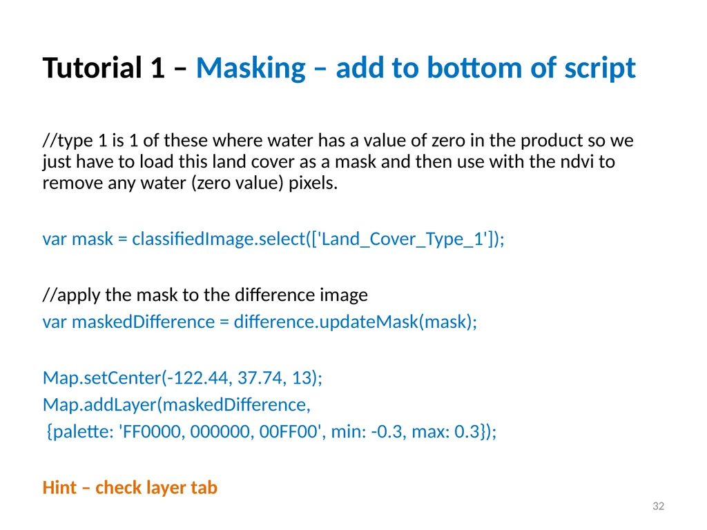
Tutorial 1 – Masking – add to bottom of script //type 1 is 1 of these where water has a value of zero in the product so we just have to load this land cover as a mask and then use with the ndvi to remove any water (zero value) pixels.
var mask = classifiedImage.select(['Land_Cover_Type_1']);
//apply the mask to the difference image
var maskedDifference = difference.updateMask(mask);
Map.setCenter(-122.44, 37.74, 13);
Map.addLayer(maskedDifference,
{palette: 'FF0000, 000000, 00FF00', min: -0.3, max: 0.3});
Hint – check layer tab 32<br>
var mask = classifiedImage.select(['Land_Cover_Type_1']);
//apply the mask to the difference image
var maskedDifference = difference.updateMask(mask);
Map.setCenter(-122.44, 37.74, 13);
Map.addLayer(maskedDifference,
{palette: 'FF0000, 000000, 00FF00', min: -0.3, max: 0.3});
Hint – check layer tab 32<br>
33
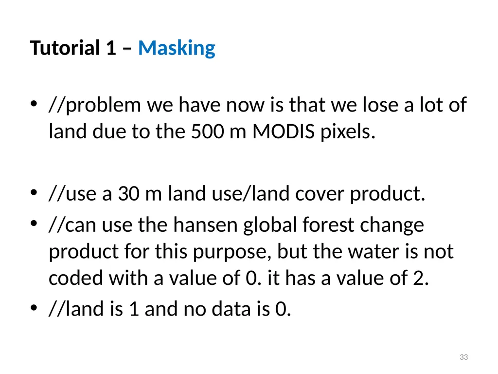
Tutorial 1 – Masking //problem we have now is that we lose a lot of land due to the 500 m MODIS pixels.
//use a 30 m land use/land cover product.
//can use the hansen global forest change product for this purpose, but the water is not coded with a value of 0. it has a value of 2.
//land is 1 and no data is 0. 33<br>
//use a 30 m land use/land cover product.
//can use the hansen global forest change product for this purpose, but the water is not coded with a value of 0. it has a value of 2.
//land is 1 and no data is 0. 33<br>
34
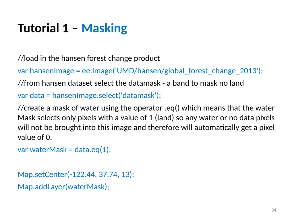
Tutorial 1 – Masking //load in the hansen forest change product
var hansenImage = ee.Image('UMD/hansen/global_forest_change_2013');
//from hansen dataset select the datamask - a band to mask no land
var data = hansenImage.select('datamask');
//create a mask of water using the operator .eq() which means that the water Mask selects only pixels with a value of 1 (land) so any water or no data pixels will not be brought into this image and therefore will automatically get a pixel value of 0.
var waterMask = data.eq(1);
Map.setCenter(-122.44, 37.74, 13);
Map.addLayer(waterMask); 34<br>
var hansenImage = ee.Image('UMD/hansen/global_forest_change_2013');
//from hansen dataset select the datamask - a band to mask no land
var data = hansenImage.select('datamask');
//create a mask of water using the operator .eq() which means that the water Mask selects only pixels with a value of 1 (land) so any water or no data pixels will not be brought into this image and therefore will automatically get a pixel value of 0.
var waterMask = data.eq(1);
Map.setCenter(-122.44, 37.74, 13);
Map.addLayer(waterMask); 34<br>
35
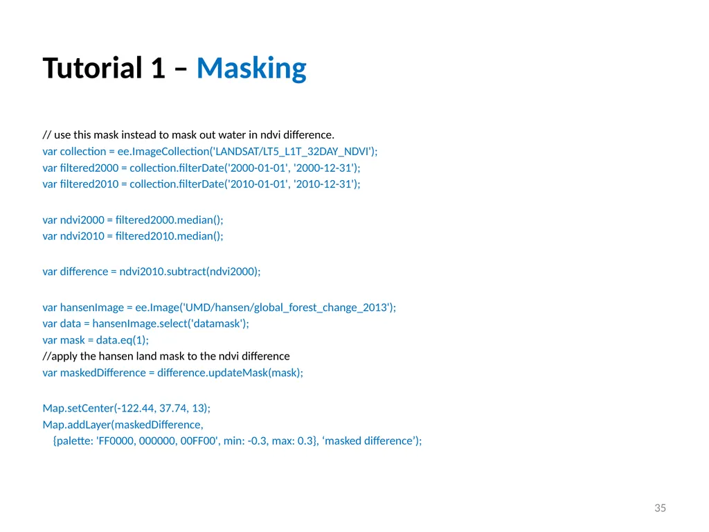
Tutorial 1 – Masking // use this mask instead to mask out water in ndvi difference.
var collection = ee.ImageCollection('LANDSAT/LT5_L1T_32DAY_NDVI');
var filtered2000 = collection.filterDate('2000-01-01', '2000-12-31');
var filtered2010 = collection.filterDate('2010-01-01', '2010-12-31');
var ndvi2000 = filtered2000.median();
var ndvi2010 = filtered2010.median();
var difference = ndvi2010.subtract(ndvi2000);
var hansenImage = ee.Image('UMD/hansen/global_forest_change_2013');
var data = hansenImage.select('datamask');
var mask = data.eq(1);
//apply the hansen land mask to the ndvi difference
var maskedDifference = difference.updateMask(mask);
Map.setCenter(-122.44, 37.74, 13);
Map.addLayer(maskedDifference,
{palette: 'FF0000, 000000, 00FF00', min: -0.3, max: 0.3}, ‘masked difference’); 35<br>
var collection = ee.ImageCollection('LANDSAT/LT5_L1T_32DAY_NDVI');
var filtered2000 = collection.filterDate('2000-01-01', '2000-12-31');
var filtered2010 = collection.filterDate('2010-01-01', '2010-12-31');
var ndvi2000 = filtered2000.median();
var ndvi2010 = filtered2010.median();
var difference = ndvi2010.subtract(ndvi2000);
var hansenImage = ee.Image('UMD/hansen/global_forest_change_2013');
var data = hansenImage.select('datamask');
var mask = data.eq(1);
//apply the hansen land mask to the ndvi difference
var maskedDifference = difference.updateMask(mask);
Map.setCenter(-122.44, 37.74, 13);
Map.addLayer(maskedDifference,
{palette: 'FF0000, 000000, 00FF00', min: -0.3, max: 0.3}, ‘masked difference’); 35<br>
36
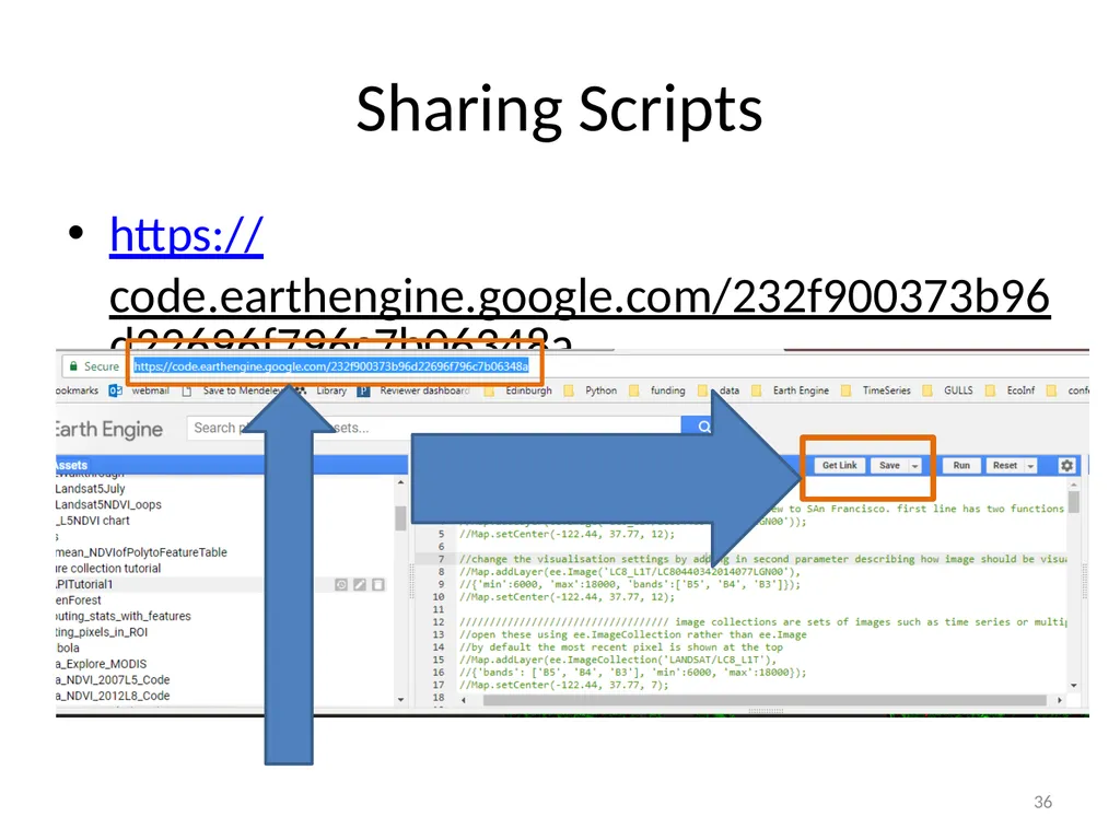
Sharing Scripts https://code.earthengine.google.com/232f900373b96d22696f796c7b06348a 36<br>
37
Review Display images
Difference between Image and ImageCollection
Simple mathemetical operators applied to images
Band math in ENVI
Filtered on date
masking 37<br>
Difference between Image and ImageCollection
Simple mathemetical operators applied to images
Band math in ENVI
Filtered on date
masking 37<br>
38
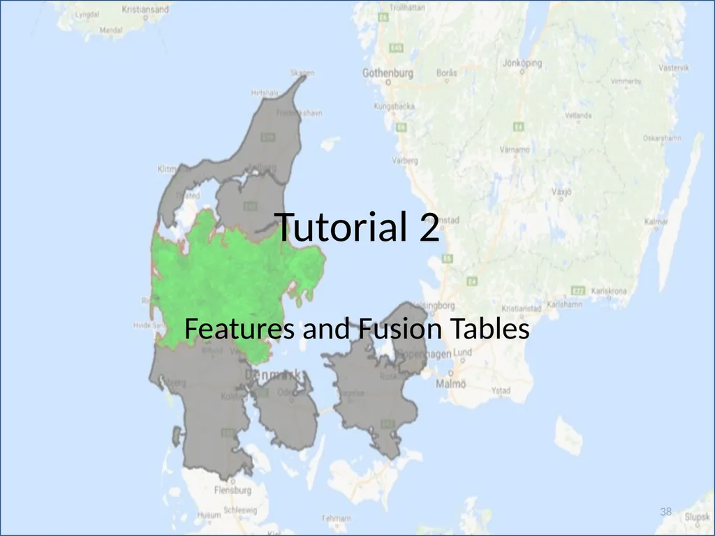
Tutorial 2 Features and Fusion Tables 38<br>
39
What is a Fusion Table? ”Experimental data visualisation web application”
Worrying?
Those familiar with GIS - Fusion tables are the way that shapefiles or polygons can be imported into EE.
Known as Feature (single) or Feature Class (multiple). 39<br>
Worrying?
Those familiar with GIS - Fusion tables are the way that shapefiles or polygons can be imported into EE.
Known as Feature (single) or Feature Class (multiple). 39<br>
40
What is a Fusion Table Can create them by importing:
Spreadsheet or delimited text file (.csv; .tsv; .txt)
KML file (google earth)
Shapeescape tool (.shp to fusion table)
Automated tool to convert into a Fusion Table. 40<br>
Spreadsheet or delimited text file (.csv; .tsv; .txt)
KML file (google earth)
Shapeescape tool (.shp to fusion table)
Automated tool to convert into a Fusion Table. 40<br>
41
Denmark Fusion Table Table ID: 1l8U580LAtM9d-fYUUfd5kRaK1BlNVZKAP8SmhEOi
This is a Fusion Table for parts of Denmark
GADM Admin Level 1 boundaries for a few places (http://gadm.org/) 41<br>
This is a Fusion Table for parts of Denmark
GADM Admin Level 1 boundaries for a few places (http://gadm.org/) 41<br>
42
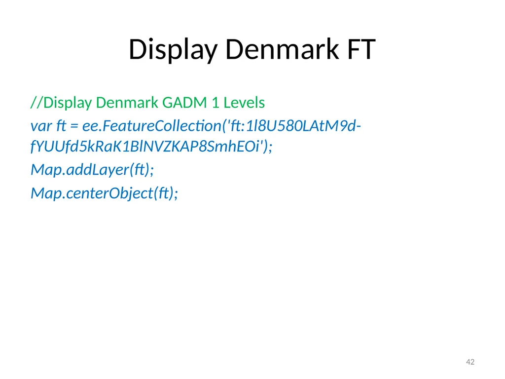
Display Denmark FT //Display Denmark GADM 1 Levels
var ft = ee.FeatureCollection('ft:1l8U580LAtM9d-fYUUfd5kRaK1BlNVZKAP8SmhEOi');
Map.addLayer(ft);
Map.centerObject(ft); 42<br>
var ft = ee.FeatureCollection('ft:1l8U580LAtM9d-fYUUfd5kRaK1BlNVZKAP8SmhEOi');
Map.addLayer(ft);
Map.centerObject(ft); 42<br>
43
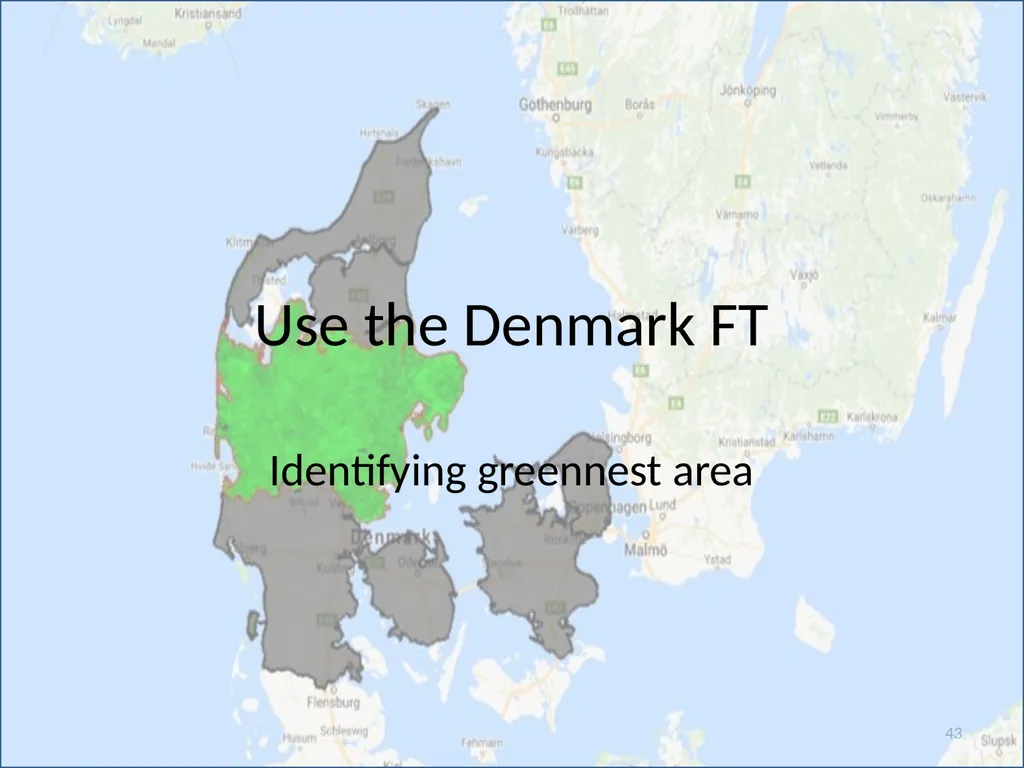
Use the Denmark FT Identifying greennest area 43<br>
44
Which Danish Area is most green? Use the fusion table in EE to find out
Average NDVI in 2015 for each Danish polygon. 44<br>
Average NDVI in 2015 for each Danish polygon. 44<br>
45
find out the median NDVI of Midtjylland in 2011 // 1. filter the feature collection
var midt = ft.filter(ee.Filter.eq('NAME_1', 'Midtjylland'));
Map.addLayer(midt, {'color':'FF0000'});
// 2. load in NDVI MODIS 16-Day Composite
var NDVI = ee.ImageCollection('MODIS/MCD43A4_NDVI').filterDate('2011-01-01','2011-12-31');
//reduce the NDVImidt to median
var median = NDVI.median(); 45<br>
var midt = ft.filter(ee.Filter.eq('NAME_1', 'Midtjylland'));
Map.addLayer(midt, {'color':'FF0000'});
// 2. load in NDVI MODIS 16-Day Composite
var NDVI = ee.ImageCollection('MODIS/MCD43A4_NDVI').filterDate('2011-01-01','2011-12-31');
//reduce the NDVImidt to median
var median = NDVI.median(); 45<br>
46
find out the median NDVI of Midtjylland in 2011 //clip to Midtjylland
var midtNDVI = median.clip(midt);
Map.addLayer(midtNDVI, {palette:'000000, 00FF00', min:0, max:0.8});
//this shows us the median pixel value in 2011 for all pixels in Midtjylland. 46<br>
var midtNDVI = median.clip(midt);
Map.addLayer(midtNDVI, {palette:'000000, 00FF00', min:0, max:0.8});
//this shows us the median pixel value in 2011 for all pixels in Midtjylland. 46<br>
47
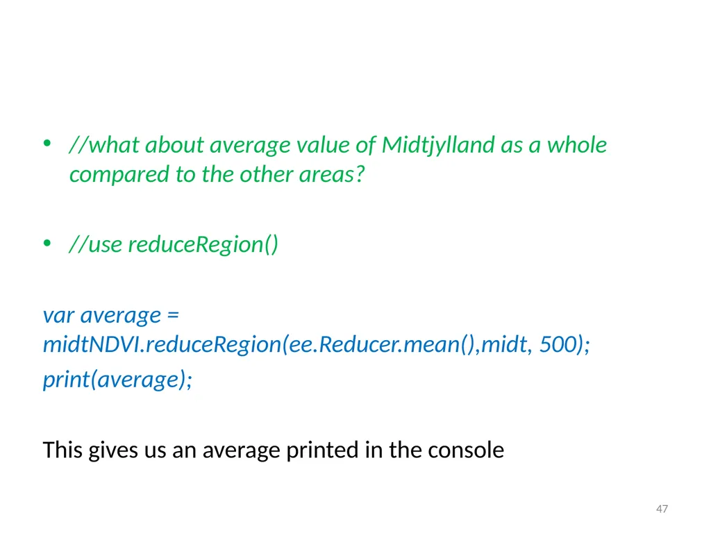
//what about average value of Midtjylland as a whole compared to the other areas?
//use reduceRegion()
var average = midtNDVI.reduceRegion(ee.Reducer.mean(),midt, 500);
print(average);
This gives us an average printed in the console 47<br>
//use reduceRegion()
var average = midtNDVI.reduceRegion(ee.Reducer.mean(),midt, 500);
print(average);
This gives us an average printed in the console 47<br>
48
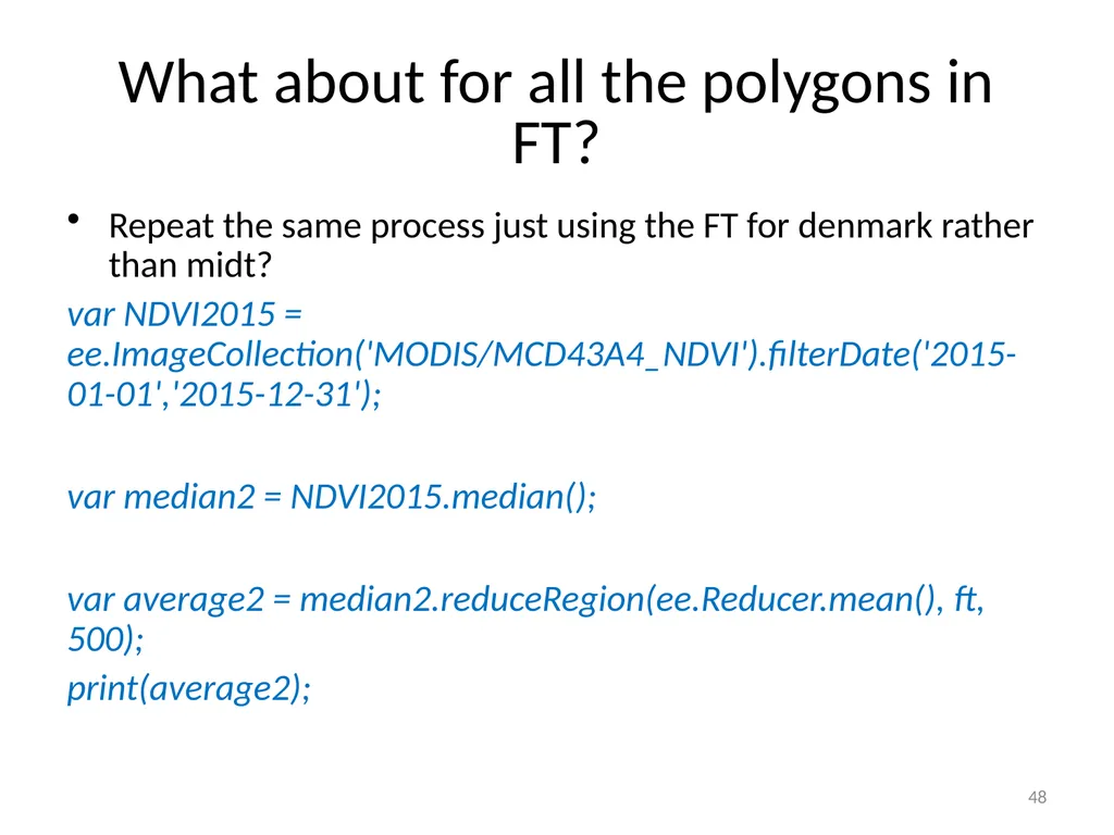
What about for all the polygons in FT? Repeat the same process just using the FT for denmark rather than midt?
var NDVI2015 = ee.ImageCollection('MODIS/MCD43A4_NDVI').filterDate('2015-01-01','2015-12-31');
var median2 = NDVI2015.median();
var average2 = median2.reduceRegion(ee.Reducer.mean(), ft, 500);
print(average2); 48<br>
var NDVI2015 = ee.ImageCollection('MODIS/MCD43A4_NDVI').filterDate('2015-01-01','2015-12-31');
var median2 = NDVI2015.median();
var average2 = median2.reduceRegion(ee.Reducer.mean(), ft, 500);
print(average2); 48<br>
49
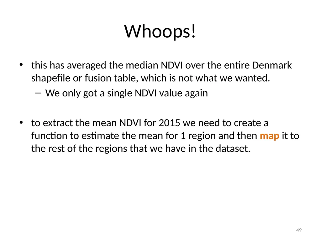
Whoops! this has averaged the median NDVI over the entire Denmark shapefile or fusion table, which is not what we wanted.
We only got a single NDVI value again
to extract the mean NDVI for 2015 we need to create a function to estimate the mean for 1 region and then map it to the rest of the regions that we have in the dataset. 49<br>
We only got a single NDVI value again
to extract the mean NDVI for 2015 we need to create a function to estimate the mean for 1 region and then map it to the rest of the regions that we have in the dataset. 49<br>
50
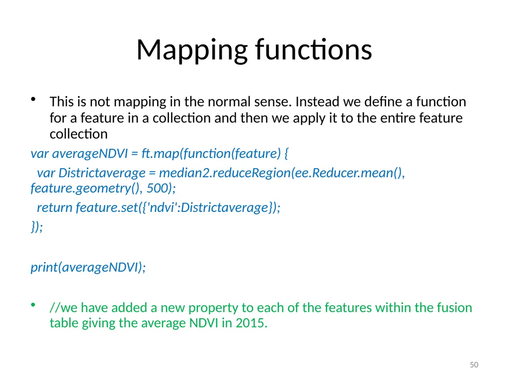
Mapping functions This is not mapping in the normal sense. Instead we define a function for a feature in a collection and then we apply it to the entire feature collection
var averageNDVI = ft.map(function(feature) {
var Districtaverage = median2.reduceRegion(ee.Reducer.mean(), feature.geometry(), 500);
return feature.set({'ndvi':Districtaverage});
});
print(averageNDVI);
//we have added a new property to each of the features within the fusion table giving the average NDVI in 2015. 50<br>
var averageNDVI = ft.map(function(feature) {
var Districtaverage = median2.reduceRegion(ee.Reducer.mean(), feature.geometry(), 500);
return feature.set({'ndvi':Districtaverage});
});
print(averageNDVI);
//we have added a new property to each of the features within the fusion table giving the average NDVI in 2015. 50<br>
51
Review Created fusion table from csv and shp file.
Uploaded and displayed in EE API
Performed basic queries on NDVI data using FT.
Wrote a Function and mapped it to a collection. 51<br>
Uploaded and displayed in EE API
Performed basic queries on NDVI data using FT.
Wrote a Function and mapped it to a collection. 51<br>
52
Comments The fusion tables are experimental – what does that mean?
There are limits to the file sizes for upload
Difficult to get polygons uploaded without using shapeescape
Difficult to create your own data in GoogleEarth and then converting it to fusion table as the geometry and name variables require specific types. 52<br>
There are limits to the file sizes for upload
Difficult to get polygons uploaded without using shapeescape
Difficult to create your own data in GoogleEarth and then converting it to fusion table as the geometry and name variables require specific types. 52<br>
53
Good to know Fusion table creation is temperamental – general advice if get errors is to try again and vary a few things:
Eg - Chrome browser doesnt always seem to work for creating fusion tables
FT’s are public. You can protect them with invite only status but you still have to upload your data onto a public google cloud
Check the data use policies before doing this!
Uploading to shapeescape could also be against data providers policies. 53<br>
Eg - Chrome browser doesnt always seem to work for creating fusion tables
FT’s are public. You can protect them with invite only status but you still have to upload your data onto a public google cloud
Check the data use policies before doing this!
Uploading to shapeescape could also be against data providers policies. 53<br>
54
Benefits of GEE? ”GEE does the same things as the software i am used to”
Uses the Google Cloud Server capabilities so the analysis is run on the fly.
You do not need to download and process gb’s of data.
Example:
NDVI time series for 12 months at 8-day repeat?
In ENVI ~ 46 images per tile
GEE – run the analysis on the 46 images without having to download. 54<br>
Uses the Google Cloud Server capabilities so the analysis is run on the fly.
You do not need to download and process gb’s of data.
Example:
NDVI time series for 12 months at 8-day repeat?
In ENVI ~ 46 images per tile
GEE – run the analysis on the 46 images without having to download. 54<br>
55
55<br>
56
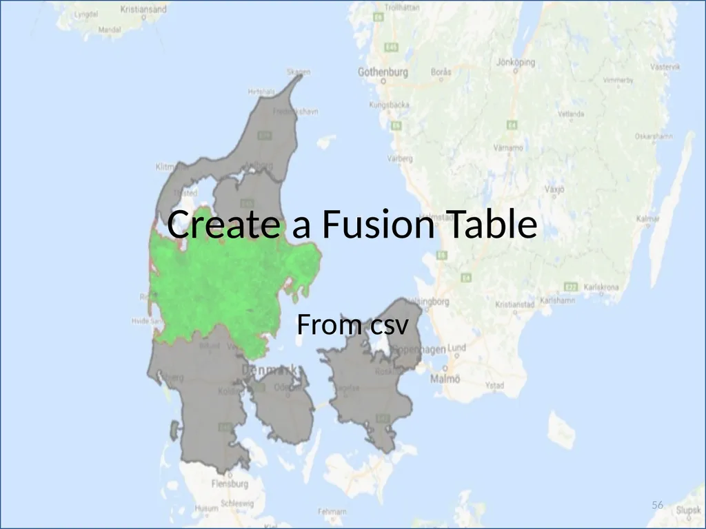
Create a Fusion Table From csv 56<br>
57
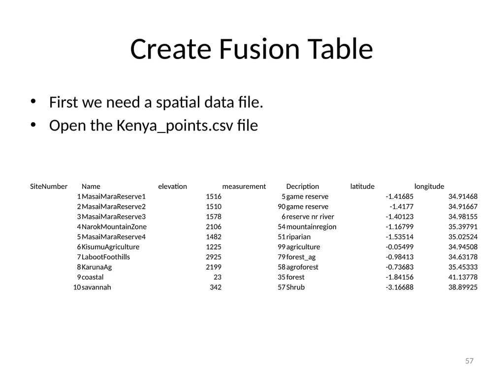
Create Fusion Table First we need a spatial data file.
Open the Kenya_points.csv file 57<br>
Open the Kenya_points.csv file 57<br>
58
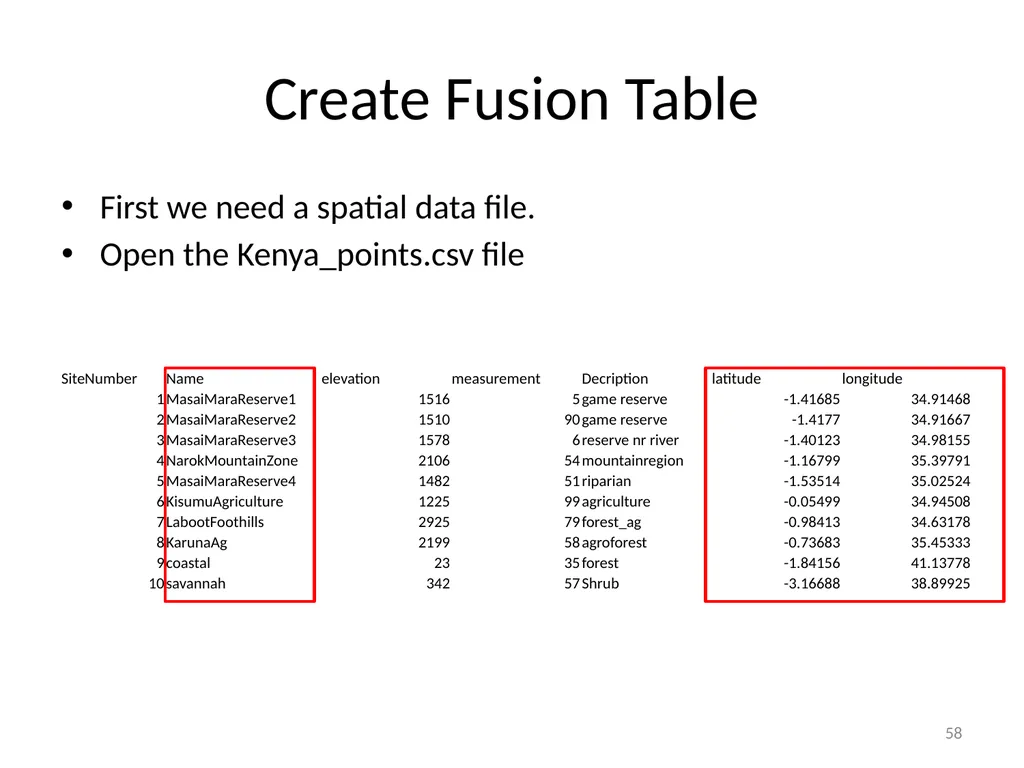
Create Fusion Table First we need a spatial data file.
Open the Kenya_points.csv file 58<br>
Open the Kenya_points.csv file 58<br>
59
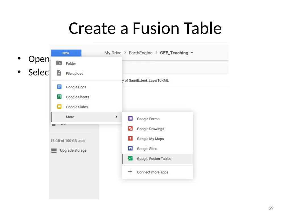
Create a Fusion Table Open Google Drive
Select new and Fusion table option 59<br>
Select new and Fusion table option 59<br>
60
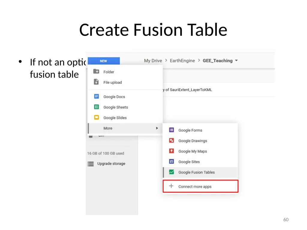
Create Fusion Table If not an option select connect more apps and search for fusion table 60<br>
61
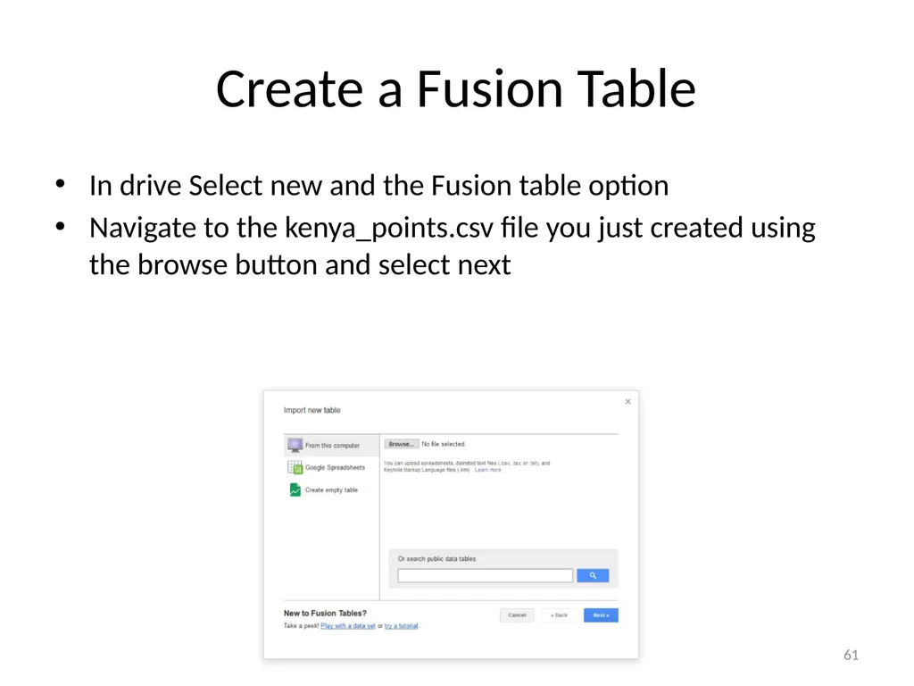
Create a Fusion Table In drive Select new and the Fusion table option
Navigate to the kenya_points.csv file you just created using the browse button and select next 61<br>
Navigate to the kenya_points.csv file you just created using the browse button and select next 61<br>
62
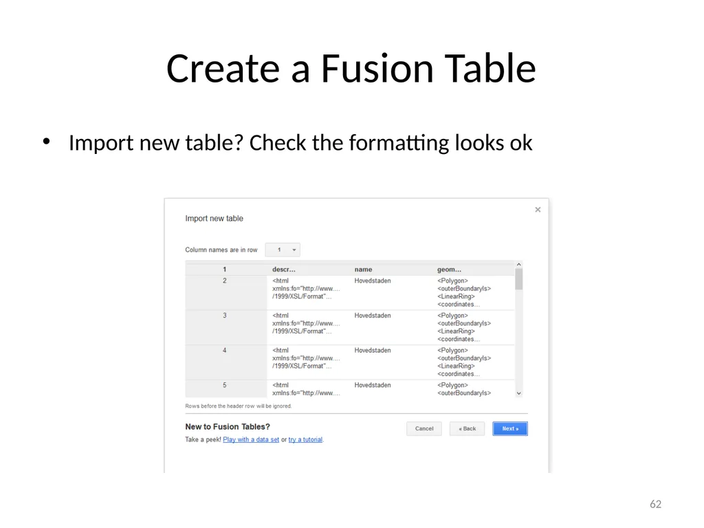
Create a Fusion Table Import new table? Check the formatting looks ok 62<br>
63
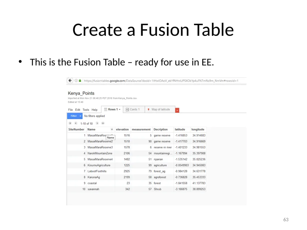
Create a Fusion Table This is the Fusion Table – ready for use in EE. 63<br>
64
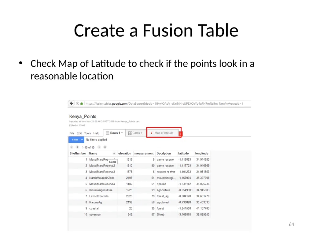
Create a Fusion Table Check Map of Latitude to check if the points look in a reasonable location 64<br>
65
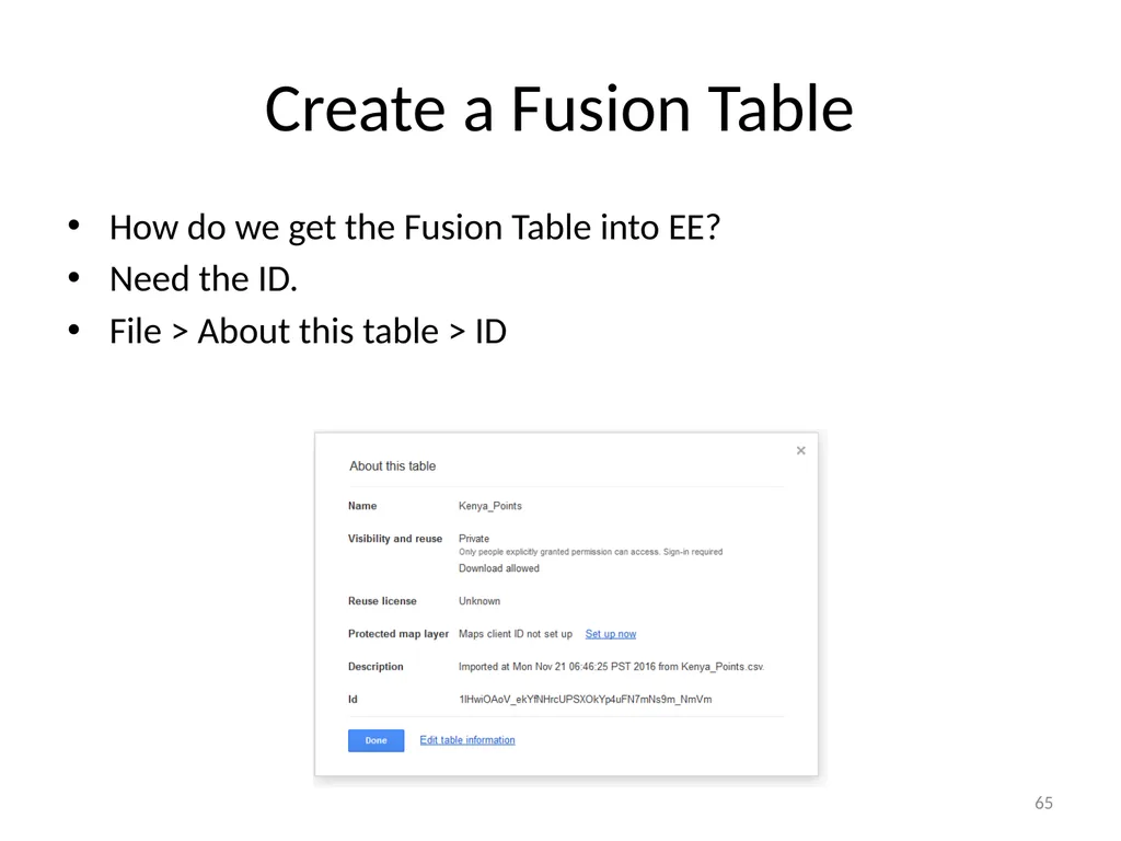
Create a Fusion Table How do we get the Fusion Table into EE?
Need the ID.
File > About this table > ID 65<br>
Need the ID.
File > About this table > ID 65<br>
66
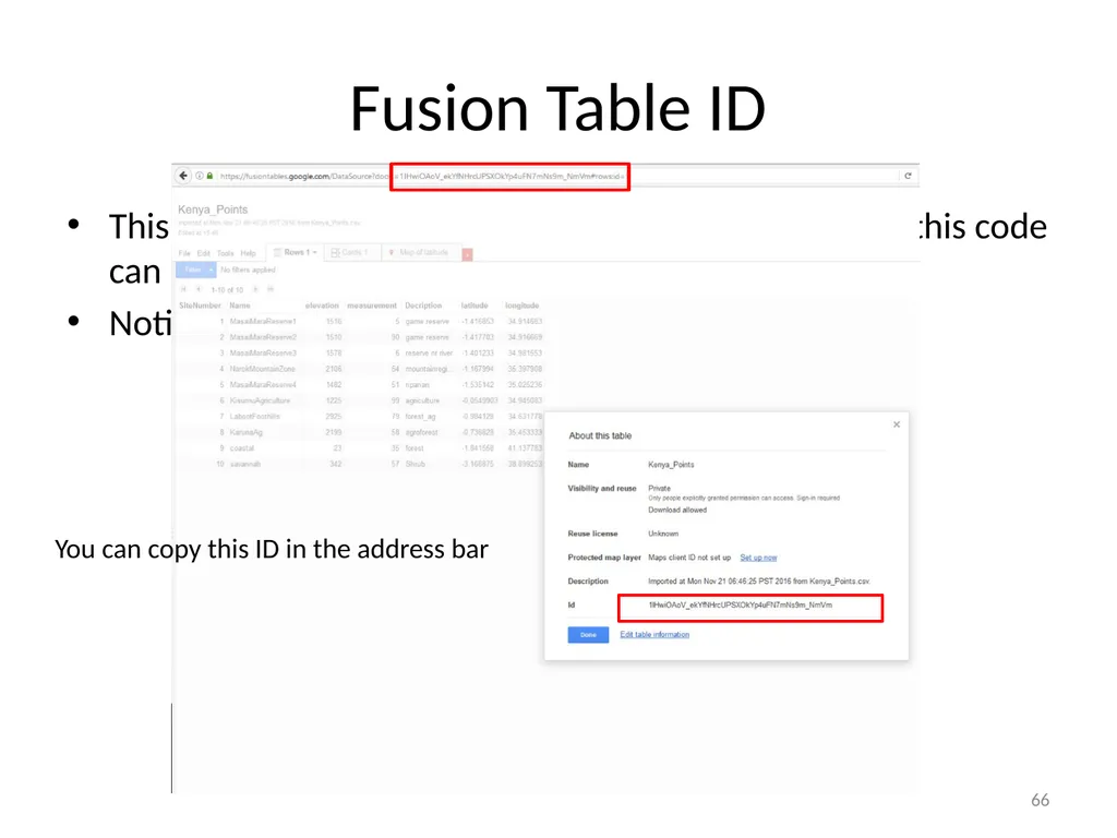
Fusion Table ID This is a unique code for your table. Anyone who has this code can access your file.
Notice that the ID also appears in the address bar You can copy this ID in the address bar 66<br>
Notice that the ID also appears in the address bar You can copy this ID in the address bar 66<br>
67
Fusion Table ID If you forget the ID? Or copy it wrong?
It is in Drive so you can always check again 67<br>
It is in Drive so you can always check again 67<br>
68
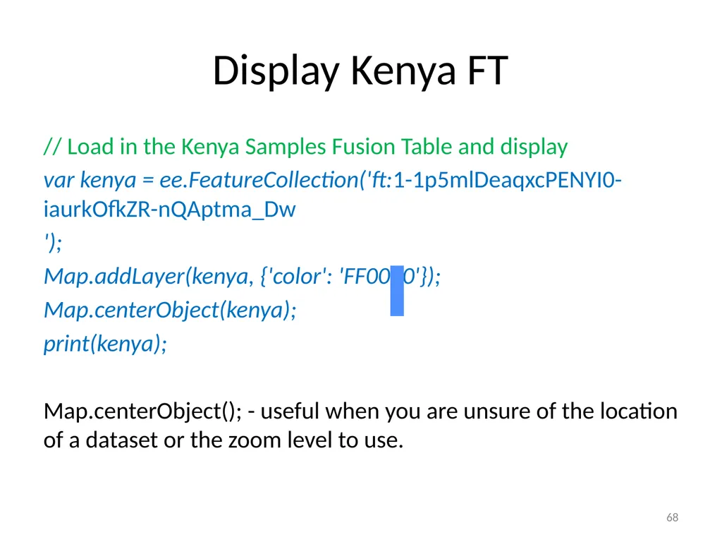
Display Kenya FT // Load in the Kenya Samples Fusion Table and display
var kenya = ee.FeatureCollection('ft:1-1p5mlDeaqxcPENYI0-iaurkOfkZR-nQAptma_Dw
');
Map.addLayer(kenya, {'color': 'FF0000'});
Map.centerObject(kenya);
print(kenya);
Map.centerObject(); - useful when you are unsure of the location of a dataset or the zoom level to use. 68<br>
var kenya = ee.FeatureCollection('ft:1-1p5mlDeaqxcPENYI0-iaurkOfkZR-nQAptma_Dw
');
Map.addLayer(kenya, {'color': 'FF0000'});
Map.centerObject(kenya);
print(kenya);
Map.centerObject(); - useful when you are unsure of the location of a dataset or the zoom level to use. 68<br>
69
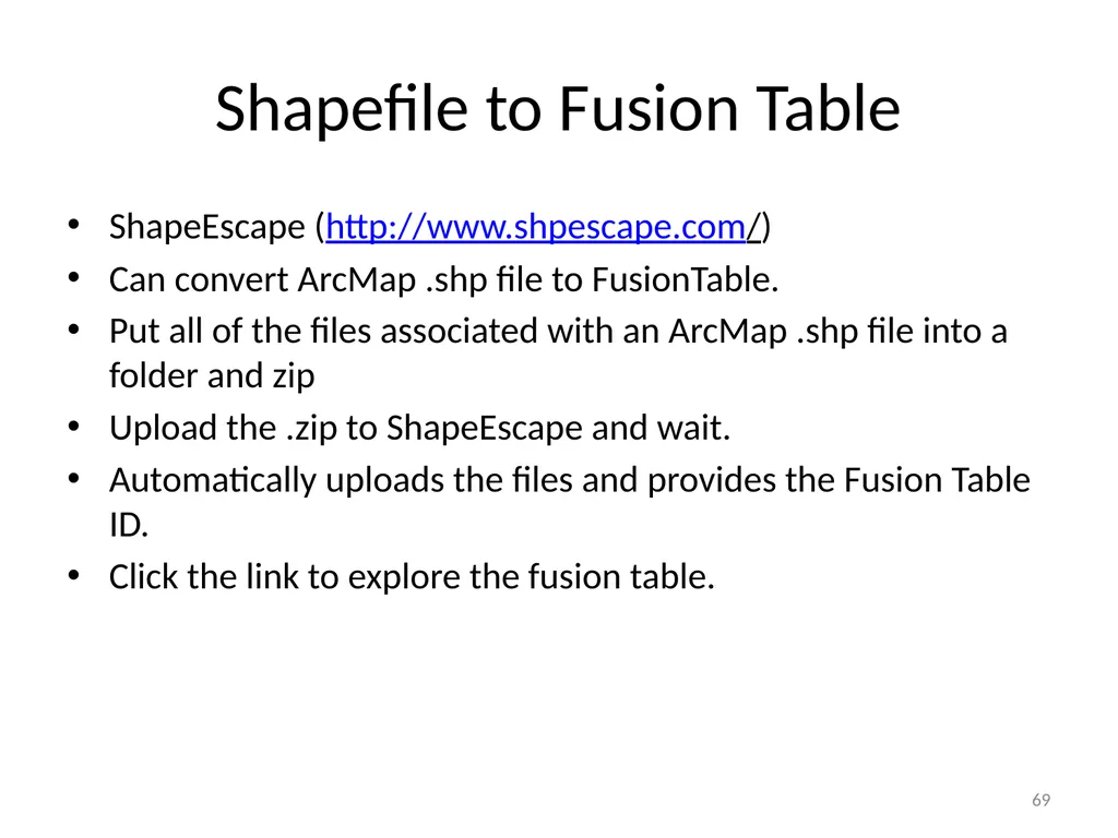
Shapefile to Fusion Table ShapeEscape (http://www.shpescape.com/)
Can convert ArcMap .shp file to FusionTable.
Put all of the files associated with an ArcMap .shp file into a folder and zip
Upload the .zip to ShapeEscape and wait.
Automatically uploads the files and provides the Fusion Table ID.
Click the link to explore the fusion table. 69<br>
Can convert ArcMap .shp file to FusionTable.
Put all of the files associated with an ArcMap .shp file into a folder and zip
Upload the .zip to ShapeEscape and wait.
Automatically uploads the files and provides the Fusion Table ID.
Click the link to explore the fusion table. 69<br>