
Introduction to Machine Learning Hayley Carr,










Description: Introduction to Machine Learning Hayley Carr, Simon Andrews, Laura Biggins hayley.carrbabraham.ac.uk v2026-03 Agenda for the day What is machine learning Different types of machine learning model Exercise Running different models How to
Related Topics
Download Presentation
"Introduction to Machine Learning Hayley Carr," is the property of its rightful owner. Permission is granted to download and print the materials on this website for personal, non-commercial use only, and to display it on your personal computer provided you do not modify the materials and that you retain all copyright notices contained in the materials. By downloading content from our website, you accept the terms of this agreement.
Presentation Transcript
slide1. Introduction to Machine Learning Hayley Carr, Simon Andrews, Laura Biggins
hayley.carr@babraham.ac.uk
v2026-03<br>
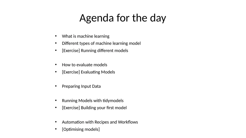
slide2. Agenda for the day What is machine learning
Different types of machine learning model
[Exercise] Running different models
How to evaluate models
[Exercise] Evaluating Models
Preparing Input Data
Running Models with tidymodels
[Exercise] Building your first model
Automation with Recipes and Workflows
[Optimising models]<br>
slide3. What is Machine Learning?<br>
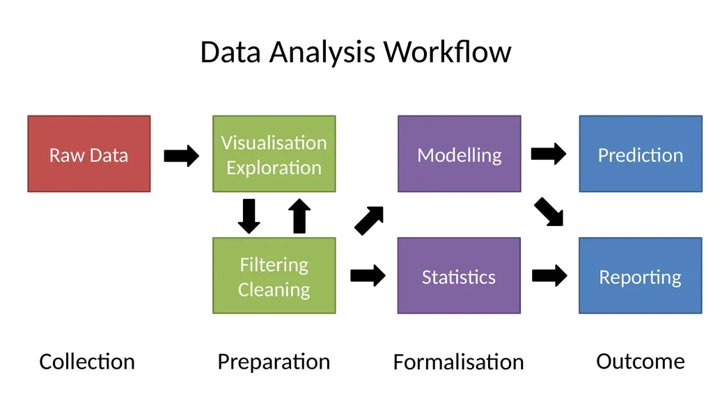
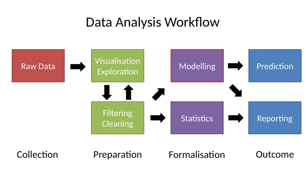
slide4. Data Analysis Workflow Raw Data Collection Preparation Formalisation Outcome<br>
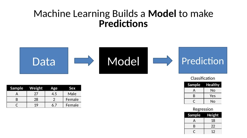
slide5. Machine Learning Builds a Model to make Predictions<br>
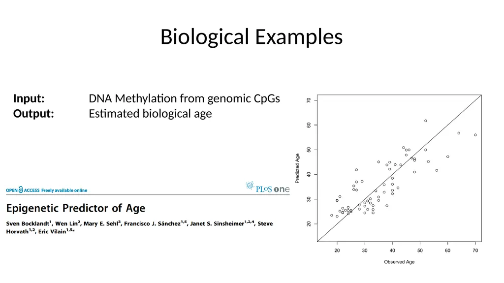
slide6. Biological Examples Input: DNA Methylation from genomic CpGs
Output: Estimated biological age<br>
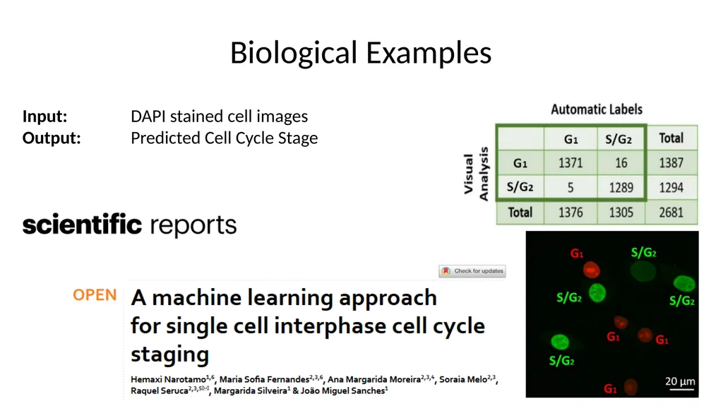
slide7. Biological Examples Input: DAPI stained cell images
Output: Predicted Cell Cycle Stage<br>
slide8. Biological Examples Input: Histopathology slide images
Output: Cancer likelihood score<br>
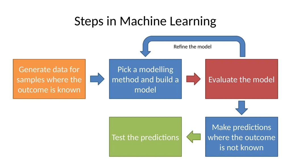
slide9. Steps in Machine Learning Generate data for samples where the outcome is known Refine the model<br>
slide10. Different machine learning models<br>
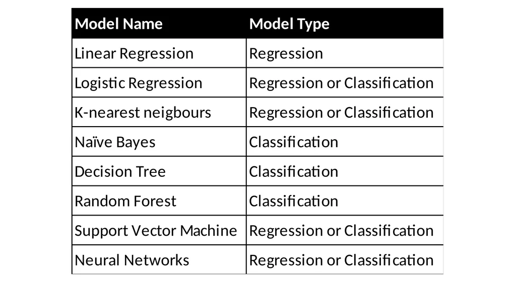
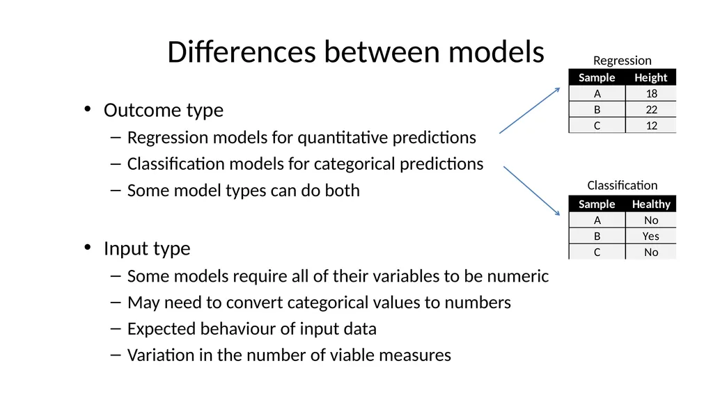
slide12. Outcome type
Regression models for quantitative predictions
Classification models for categorical predictions
Some model types can do both
Input type
Some models require all of their variables to be numeric
May need to convert categorical values to numbers
Expected behaviour of input data
Variation in the number of viable measures Differences between models<br>
slide13. K-Nearest Neighbours (KNN) models<br>
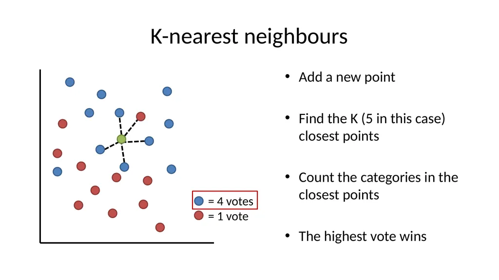
slide14. K-nearest neighbours Add a new point
Find the K (5 in this case) closest points
Count the categories in the closest points
The highest vote wins<br>
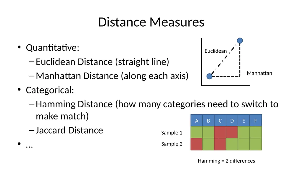
slide15. Distance Measures Quantitative:
Euclidean Distance (straight line)
Manhattan Distance (along each axis)
Categorical:
Hamming Distance (how many categories need to switch to make match)
Jaccard Distance
… Manhattan Euclidean Sample 1 Sample 2 Hamming = 2 differences<br>
slide16. Support Vector Machine (SVM) models<br>
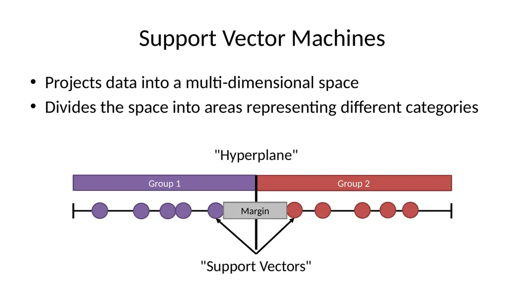
slide17. Support Vector Machines Projects data into a multi-dimensional space
Divides the space into areas representing different categories "Hyperplane" Margin<br>
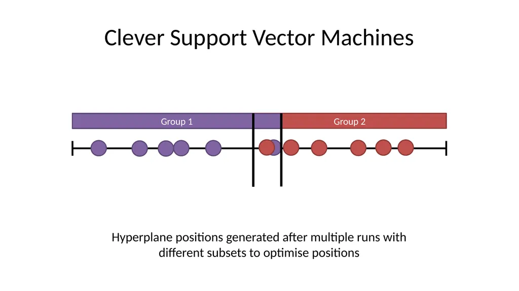
slide18. Group 2 Group 1 Clever Support Vector Machines Hyperplane positions generated after multiple runs with different subsets to optimise positions<br>
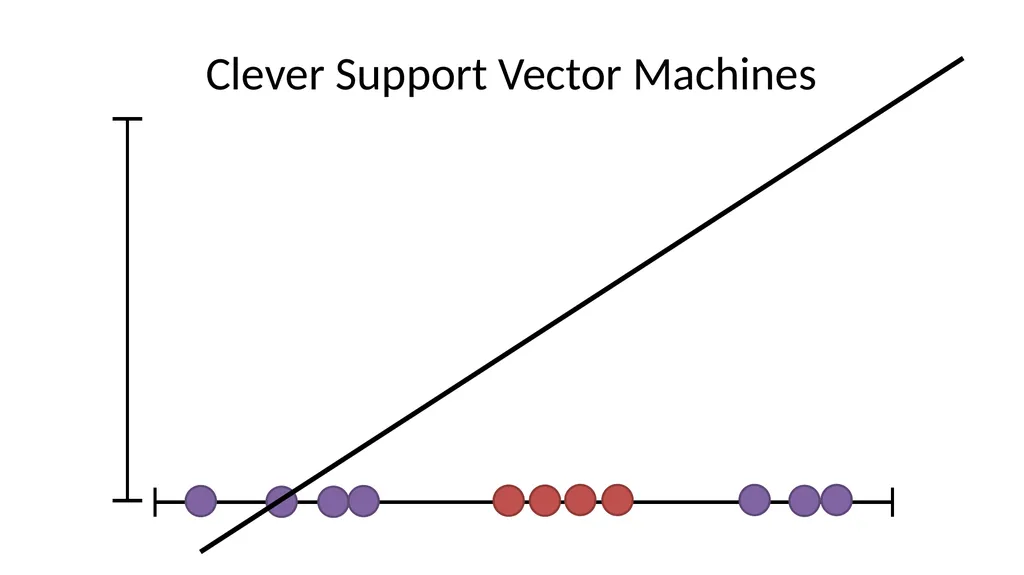
slide19. Clever Support Vector Machines<br>
slide20. Support Vector Machines Project data into higher dimensions find a support vector classifier that divides groups
Can use or define different kernel functions
Differ in how they “transform” data/how they define threshold
Previous slide = polynomial, second degree (squared values)<br>
slide21. Naïve Bayes Models<br>
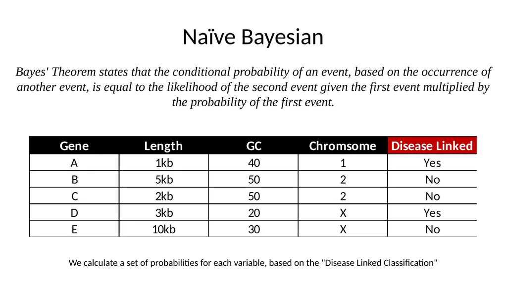
slide22. Naïve Bayesian Bayes' Theorem states that the conditional probability of an event, based on the occurrence of another event, is equal to the likelihood of the second event given the first event multiplied by the probability of the first event. We calculate a set of probabilities for each variable, based on the "Disease Linked Classification"<br>
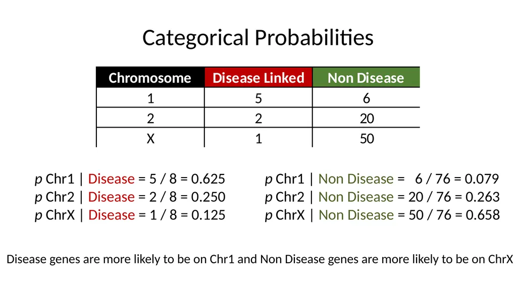
slide23. Categorical Probabilities p Chr1 | Disease = 5 / 8 = 0.625
p Chr2 | Disease = 2 / 8 = 0.250
p ChrX | Disease = 1 / 8 = 0.125 p Chr1 | Non Disease = 6 / 76 = 0.079
p Chr2 | Non Disease = 20 / 76 = 0.263
p ChrX | Non Disease = 50 / 76 = 0.658 Disease genes are more likely to be on Chr1 and Non Disease genes are more likely to be on ChrX<br>
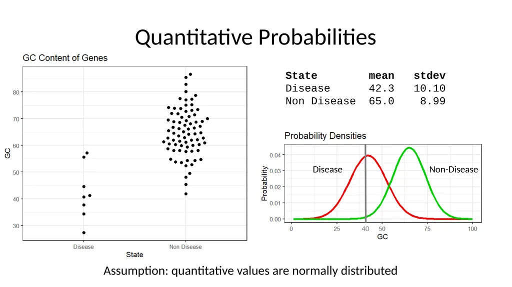
slide24. Quantitative Probabilities State mean stdev
Disease 42.3 10.10
Non Disease 65.0 8.99 Assumption: quantitative values are normally distributed<br>
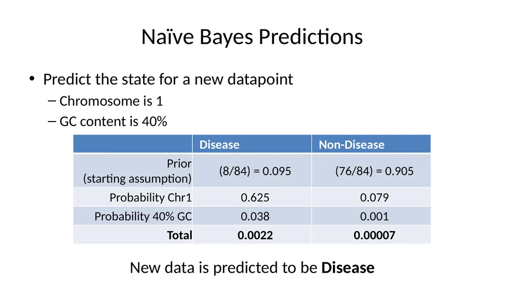
slide25. Naïve Bayes Predictions Predict the state for a new datapoint
Chromosome is 1
GC content is 40% New data is predicted to be Disease Non -<br>
slide26. Decision Trees<br>
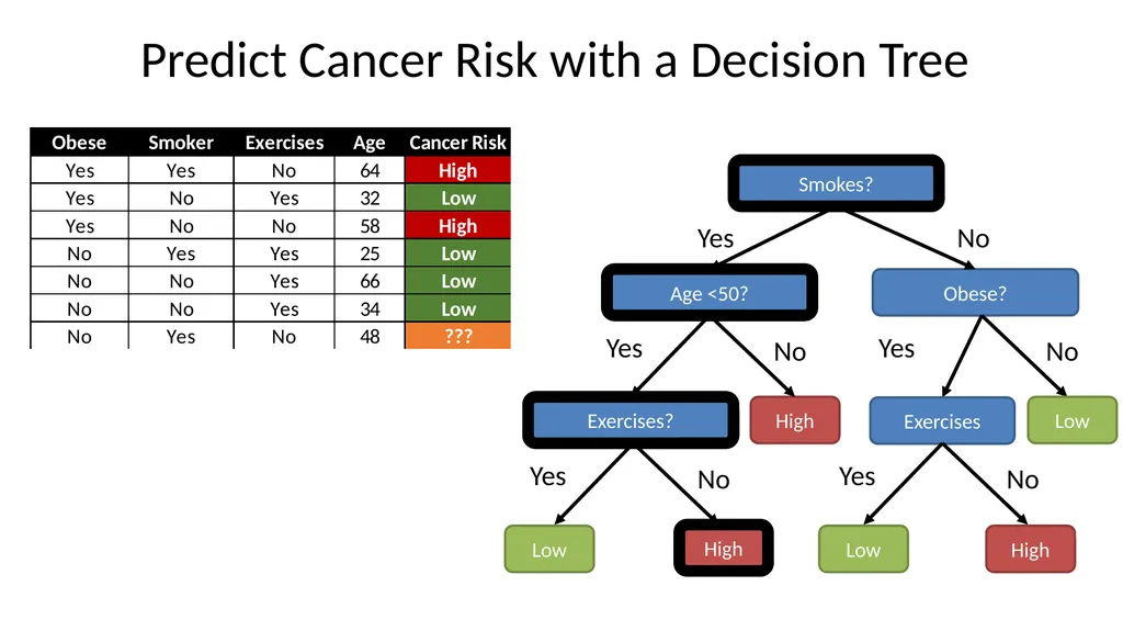
slide27. Predict Cancer Risk with a Decision Tree Smokes? Age <50? Exercises? High<br>
slide28. How do you build a tree? From a population of observations
Which variable do you use when?
[If quantitative] which cutoff do you use?
Answer: you calculate an ‘impurity’ score and pick the least ‘impure’ variable to split the remaining data
Want to use the most cleanly predictive question to improve the tree<br>
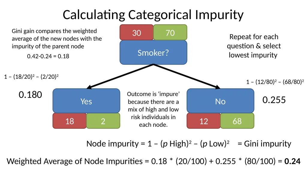
slide29. Calculating Categorical Impurity Smoker? 30 70 Outcome is ‘impure’ because there are a mix of high and low risk individuals in each node. Node impurity = 1 – (p High)2 – (p Low)2 1 – (18/20)2 – (2/20)2
0.180 1 – (12/80)2 – (68/80)2
0.255 Weighted Average of Node Impurities = 0.18 * (20/100) + 0.255 * (80/100) = 0.24 Repeat for each question & select lowest impurity = Gini impurity Gini gain compares the weighted average of the new nodes with the impurity of the parent node 0.42-0.24 = 0.18<br>
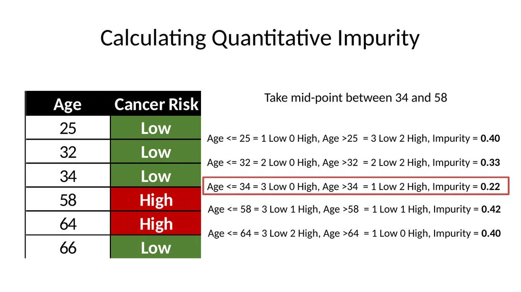
slide30. Calculating Quantitative Impurity Take mid-point between 34 and 58<br>
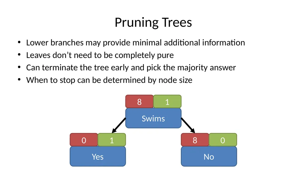
slide31. Pruning Trees Lower branches may provide minimal additional information
Leaves don’t need to be completely pure
Can terminate the tree early and pick the majority answer
When to stop can be determined by node size<br>
slide32. Random Forests<br>
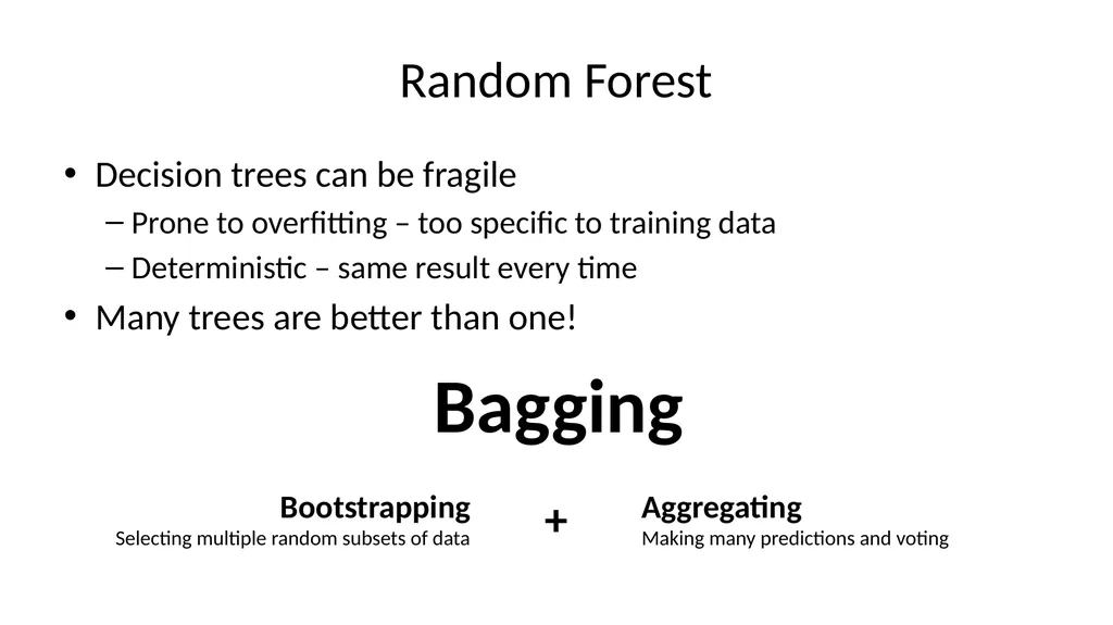
slide33. Random Forest Decision trees can be fragile
Prone to overfitting – too specific to training data
Deterministic – same result every time
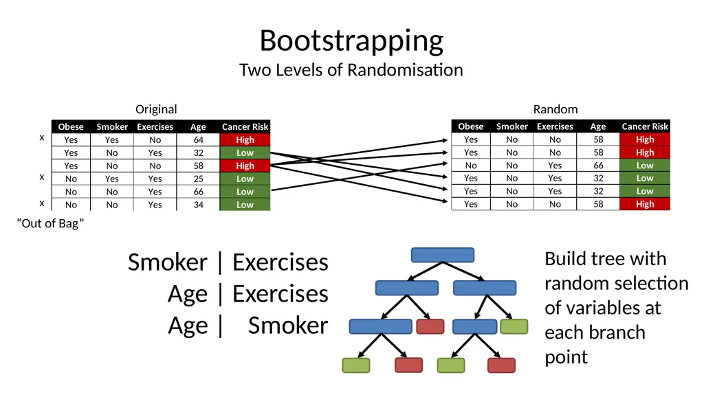
Many trees are better than one! Bagging Bootstrapping
Selecting multiple random subsets of data<br>
slide34. Bootstrapping Two Levels of Randomisation Smoker | Exercises
Age | Exercises
Age | Smoker<br>
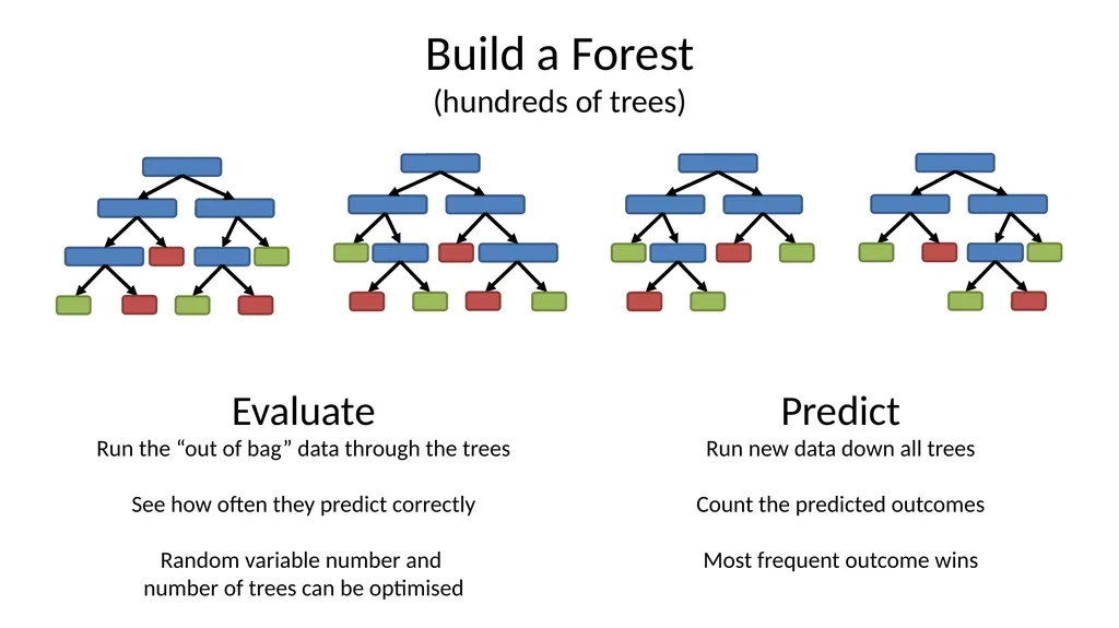
slide35. Build a Forest (hundreds of trees) Evaluate
Run the “out of bag” data through the trees
See how often they predict correctly
Random variable number and
number of trees can be optimised Predict
Run new data down all trees
Count the predicted outcomes
Most frequent outcome wins<br>
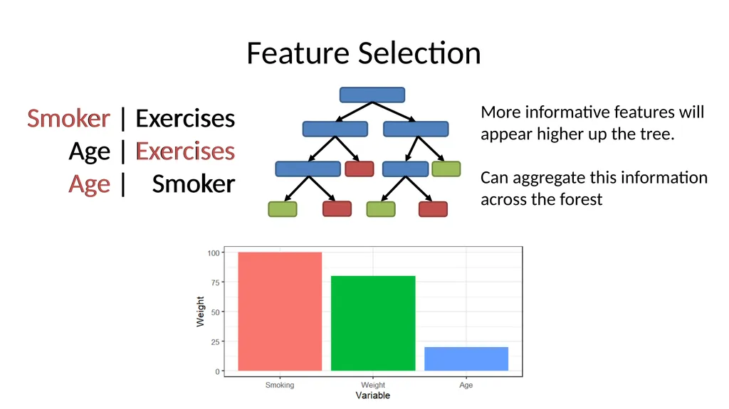
slide36. Feature Selection Smoker | Exercises
Age | Exercises
Age | Smoker Smoker | Exercises
Age | Exercises
Age | Smoker More informative features will appear higher up the tree.
Can aggregate this information across the forest<br>
slide37. Neural Networks<br>
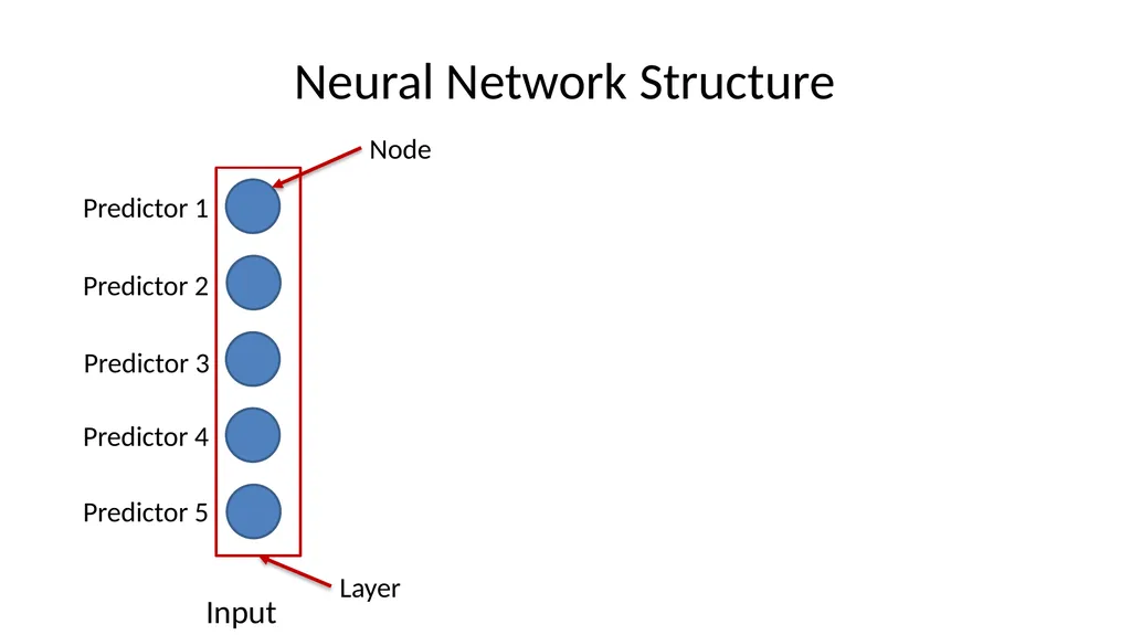
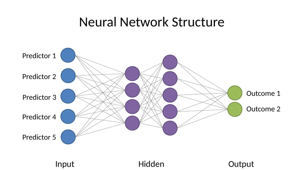
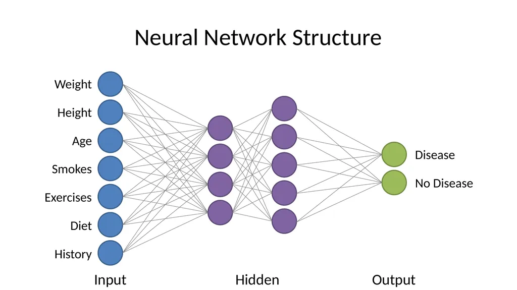
slide38. Neural Network Structure Input Node Layer<br>
slide39. Neural Network Structure Input Hidden Output<br>
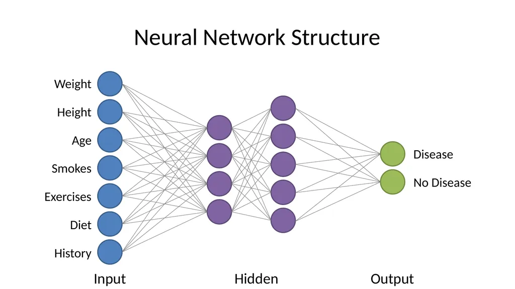
slide40. Neural Network Structure Input Hidden Output<br>
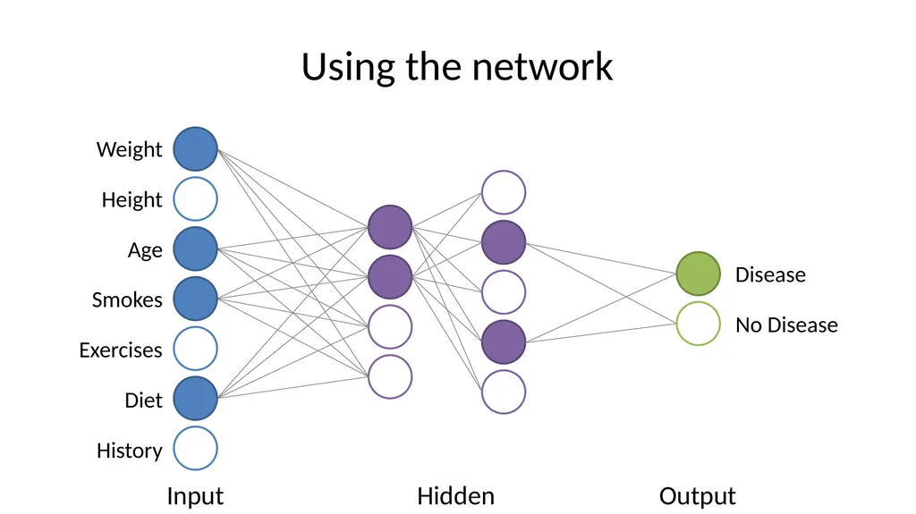
slide41. Using the network Hidden Output Input<br>
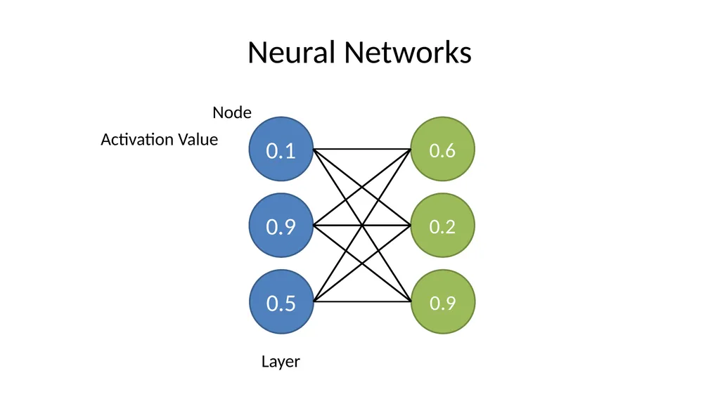
slide42. Neural Networks 0.1 0.9 0.5 Node Layer 0.6 0.2 0.9 Activation Value<br>
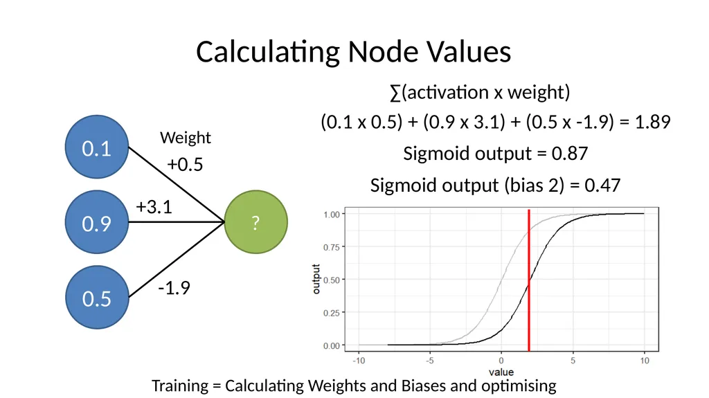
slide43. Calculating Node Values 0.1 0.9 0.5 ? +0.5 +3.1 -1.9 Weight (0.1 x 0.5) + (0.9 x 3.1) + (0.5 x -1.9) = 1.89 Sigmoid output = 0.87 Sigmoid output (bias 2) = 0.47 Training = Calculating Weights and Biases and optimising ∑(activation x weight)<br>
slide44. Neural Network Structure Input Hidden Output<br>
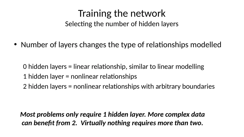
slide45. Training the network Selecting the number of hidden layers Number of layers changes the type of relationships modelled
0 hidden layers = linear relationship, similar to linear modelling
1 hidden layer = nonlinear relationships
2 hidden layers = nonlinear relationships with arbitrary boundaries Most problems only require 1 hidden layer. More complex data can benefit from 2. Virtually nothing requires more than two.<br>
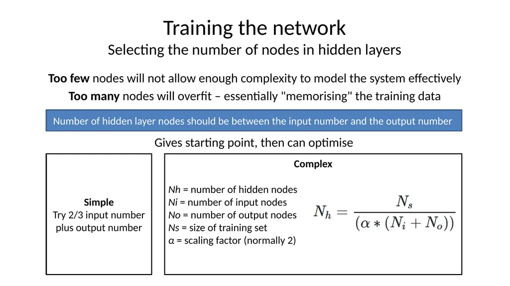
slide46. Training the network Selecting the number of nodes in hidden layers Too few nodes will not allow enough complexity to model the system effectively
Too many nodes will overfit – essentially "memorising" the training data Number of hidden layer nodes should be between the input number and the output number Simple
Try 2/3 input number plus output number Complex
Nh = number of hidden nodes
Ni = number of input nodes
No = number of output nodes
Ns = size of training set
α = scaling factor (normally 2) Gives starting point, then can optimise<br>
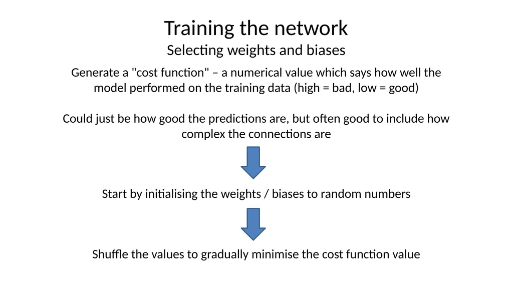
slide47. Training the network Selecting weights and biases Generate a "cost function" – a numerical value which says how well the model performed on the training data (high = bad, low = good)
Could just be how good the predictions are, but often good to include how complex the connections are<br>
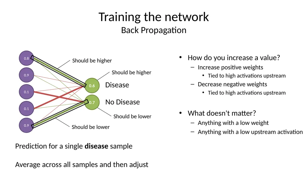
slide48. Training the network Back Propagation How do you increase a value?
Increase positive weights
Tied to high activations upstream
Decrease negative weights
Tied to high activations upstream
What doesn't matter?
Anything with a low weight
Anything with a low upstream activation Disease No Disease Prediction for a single disease sample
Average across all samples and then adjust Should be lower 0.6 0.7<br>
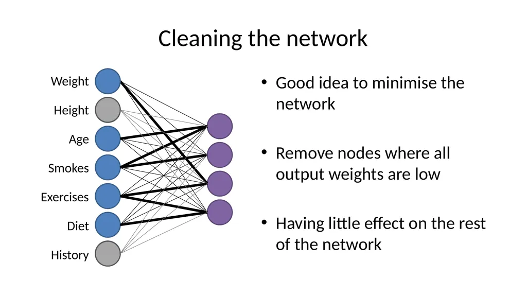
slide49. Cleaning the network Good idea to minimise the network
Remove nodes where all output weights are low
Having little effect on the rest of the network<br>
slide50. Exercise: Trying different models<br>
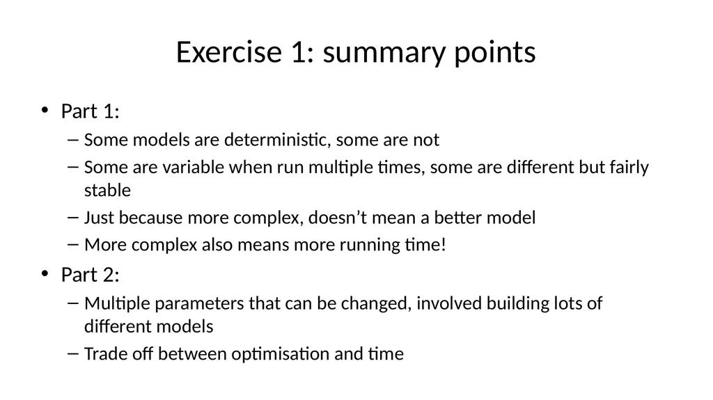
slide51. Exercise 1: summary points Part 1:
Some models are deterministic, some are not
Some are variable when run multiple times, some are different but fairly stable
Just because more complex, doesn’t mean a better model
More complex also means more running time!
Part 2:
Multiple parameters that can be changed, involved building lots of different models
Trade off between optimisation and time<br>
slide52. Evaluating Models<br>
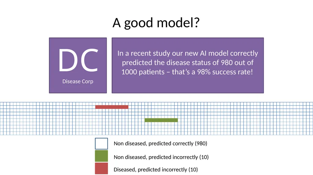
slide53. A good model?<br>
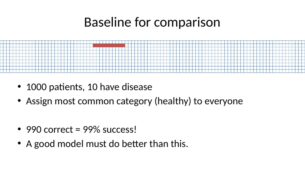
slide54. Baseline for comparison 1000 patients, 10 have disease
Assign most common category (healthy) to everyone
990 correct = 99% success!
A good model must do better than this.<br>
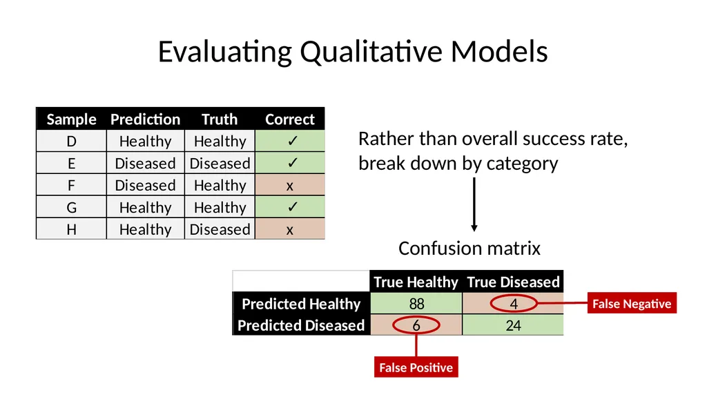
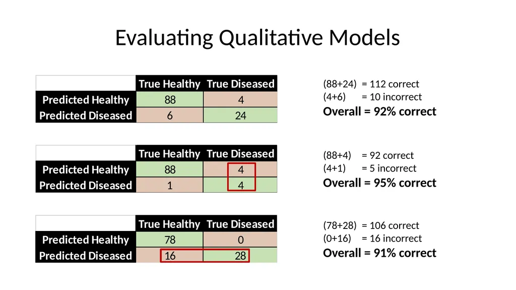
slide55. Evaluating Qualitative Models Rather than overall success rate, break down by category Confusion matrix<br>
slide56. Evaluating Qualitative Models (88+24) = 112 correct
(4+6) = 10 incorrect
Overall = 92% correct (88+4) = 92 correct
(4+1) = 5 incorrect
Overall = 95% correct (78+28) = 106 correct
(0+16) = 16 incorrect
Overall = 91% correct<br>
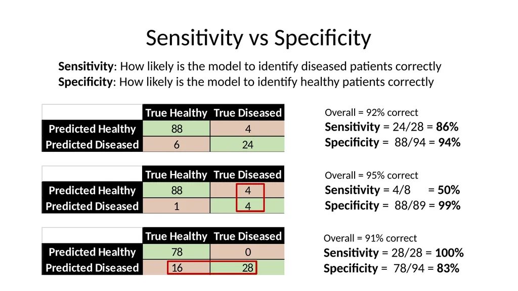
slide57. Sensitivity vs Specificity Overall = 92% correct
Sensitivity = 24/28 = 86%
Specificity = 88/94 = 94% Sensitivity: How likely is the model to identify diseased patients correctly
Specificity: How likely is the model to identify healthy patients correctly Overall = 95% correct
Sensitivity = 4/8 = 50%
Specificity = 88/89 = 99% Overall = 91% correct
Sensitivity = 28/28 = 100%
Specificity = 78/94 = 83%<br>
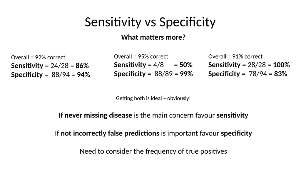
slide58. Sensitivity vs Specificity What matters more? Overall = 92% correct
Sensitivity = 24/28 = 86%
Specificity = 88/94 = 94% Overall = 95% correct
Sensitivity = 4/8 = 50%
Specificity = 88/89 = 99% Overall = 91% correct
Sensitivity = 28/28 = 100%
Specificity = 78/94 = 83% Getting both is ideal – obviously!
If never missing disease is the main concern favour sensitivity
If not incorrectly false predictions is important favour specificity
Need to consider the frequency of true positives<br>
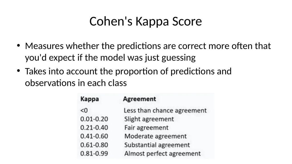
slide59. Cohen's Kappa Score Measures whether the predictions are correct more often that you'd expect if the model was just guessing
Takes into account the proportion of predictions and observations in each class<br>
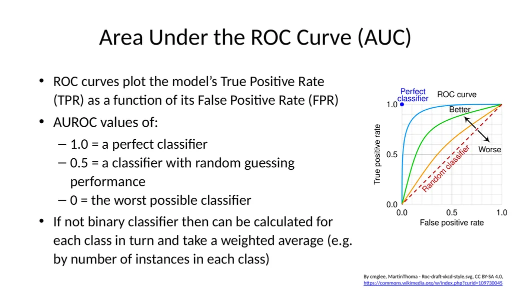
slide60. Area Under the ROC Curve (AUC) ROC curves plot the model’s True Positive Rate (TPR) as a function of its False Positive Rate (FPR)
AUROC values of:
1.0 = a perfect classifier
0.5 = a classifier with random guessing performance
0 = the worst possible classifier
If not binary classifier then can be calculated for each class in turn and take a weighted average (e.g. by number of instances in each class) By cmglee, MartinThoma - Roc-draft-xkcd-style.svg, CC BY-SA 4.0, https://commons.wikimedia.org/w/index.php?curid=109730045<br>
slide61. Evaluating Quantitative Models Correlation/association between predictions and true values (R or R2)
How close are the predictions to the true values?
Doesn’t matter if the mistake is high or low
Need a single value to summarise the total error<br>
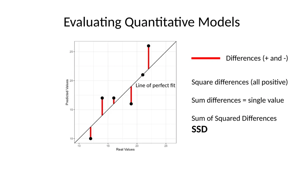
slide62. Evaluating Quantitative Models Line of perfect fit Square differences (all positive)
Sum differences = single value
Sum of Squared Differences
SSD<br>
slide63. Exercise: Evaluating Models<br>
slide64. Making best use of your data when building and testing models<br>
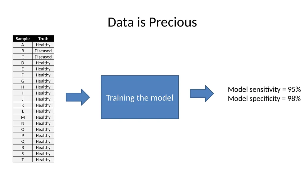
slide65. Data is Precious<br>
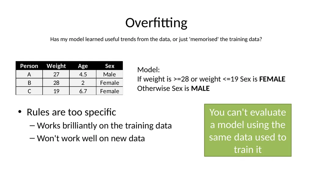
slide66. Overfitting Rules are too specific
Works brilliantly on the training data
Won't work well on new data Has my model learned useful trends from the data, or just 'memorised' the training data? Model:
If weight is >=28 or weight <=19 Sex is FEMALE
Otherwise Sex is MALE You can't evaluate a model using the same data used to train it<br>
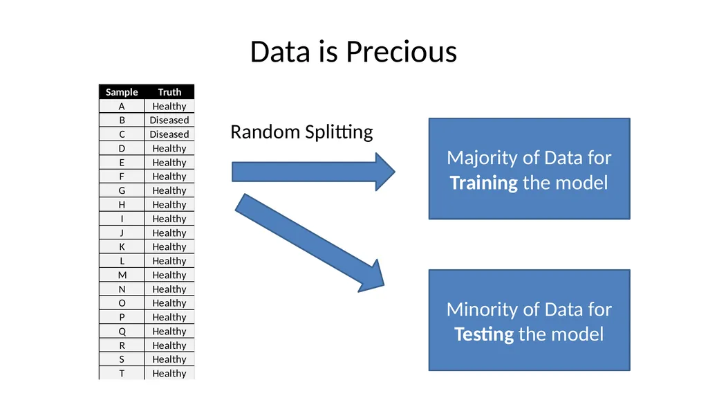
slide67. Data is Precious Random Splitting<br>
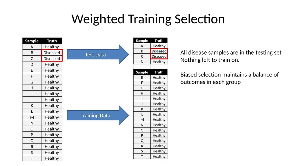
slide68. Weighted Training Selection All disease samples are in the testing set
Nothing left to train on.
Biased selection maintains a balance of outcomes in each group<br>
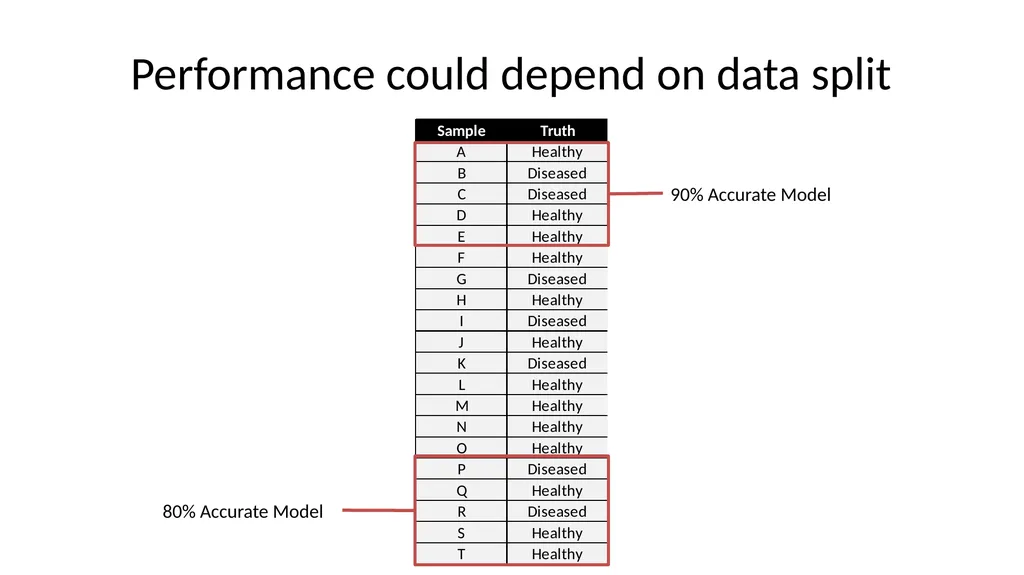
slide69. Performance could depend on data split 90% Accurate Model 80% Accurate Model<br>
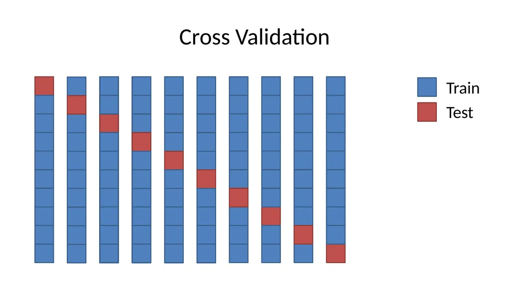
slide70. Cross Validation<br>
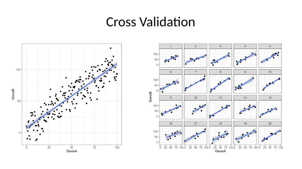
slide71. Cross Validation<br>
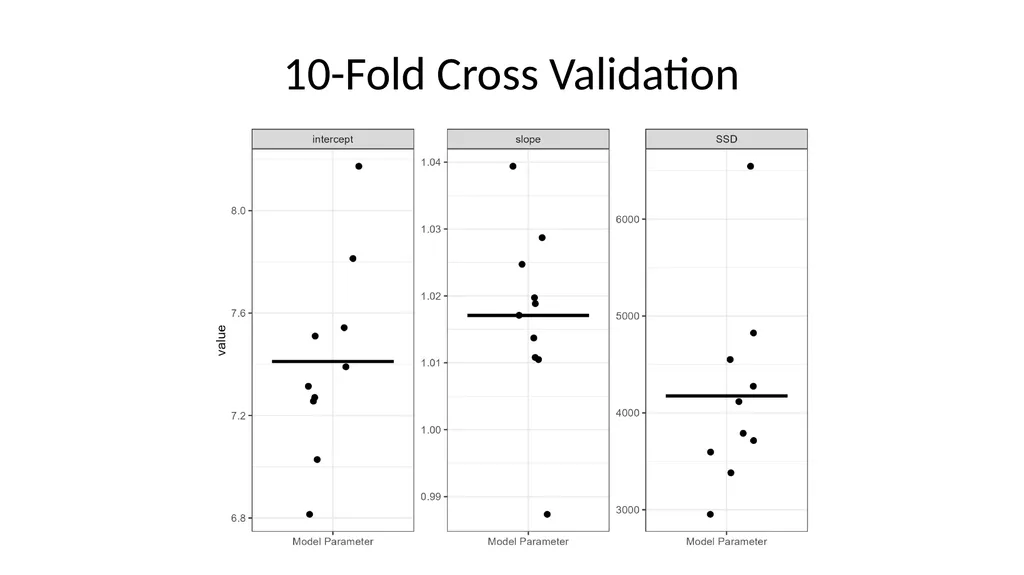
slide72. 10-Fold Cross Validation<br>
slide73. Input Data<br>
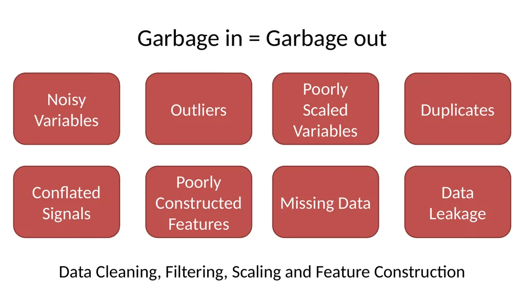
slide74. Garbage in = Garbage out Data Cleaning, Filtering, Scaling and Feature Construction<br>
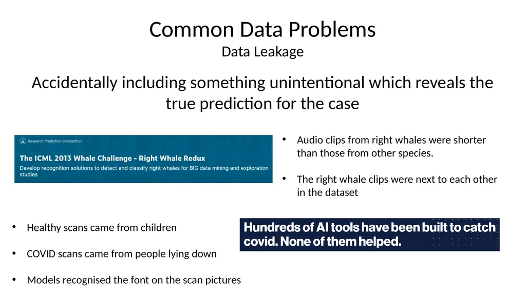
slide75. Common Data Problems Data Leakage Accidentally including something unintentional which reveals the true prediction for the case Audio clips from right whales were shorter than those from other species.
The right whale clips were next to each other in the dataset Healthy scans came from children
COVID scans came from people lying down
Models recognised the font on the scan pictures<br>
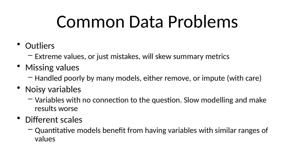
slide76. Common Data Problems Outliers
Extreme values, or just mistakes, will skew summary metrics
Missing values
Handled poorly by many models, either remove, or impute (with care)
Noisy variables
Variables with no connection to the question. Slow modelling and make results worse
Different scales
Quantitative models benefit from having variables with similar ranges of values<br>
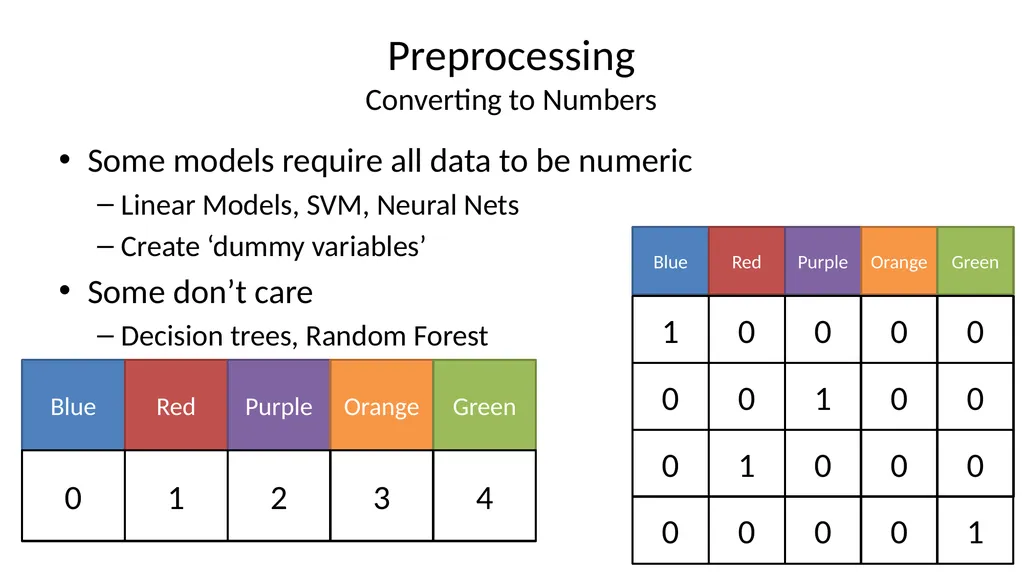
slide77. Preprocessing Converting to Numbers Some models require all data to be numeric
Linear Models, SVM, Neural Nets
Create ‘dummy variables’
Some don’t care
Decision trees, Random Forest<br>
slide78. Pre-processing Some models cannot use categorical data as input – create a dummy variable
Converted original sequence data to digital matrix for SVM model input:
‘A’ = [1, 0, 0, 0]; ‘G’ = [0, 1, 0, 0]; ‘C’ = [0, 0, 1, 0]; ‘T’ = [0, 0, 0, 1]
E.g. ‘AGT’ becomes [1, 0, 0, 0, 0, 1, 0, 0, 0, 0, 0, 1]
Can alternatively have a ‘baseline’ value, e.g.:
A = [0, 0 ,0]; G = [1, 0, 0]; C = [0, 1, 0]; T = [0, 0, 1] One-hot encoding<br>
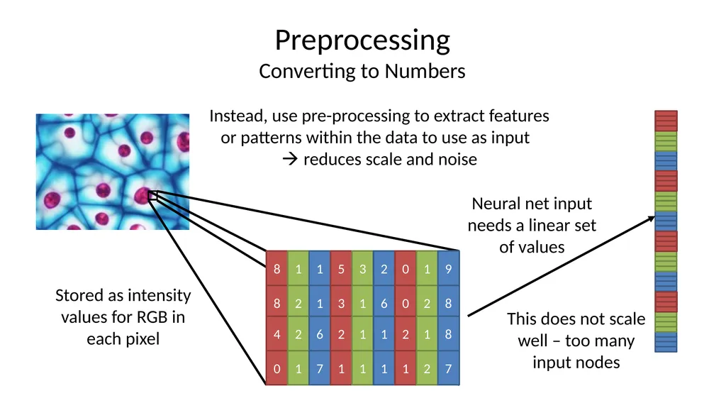
slide79. Preprocessing Converting to Numbers Stored as intensity values for RGB in each pixel Neural net input needs a linear set of values This does not scale well – too many input nodes Instead, use pre-processing to extract features or patterns within the data to use as input
reduces scale and noise<br>
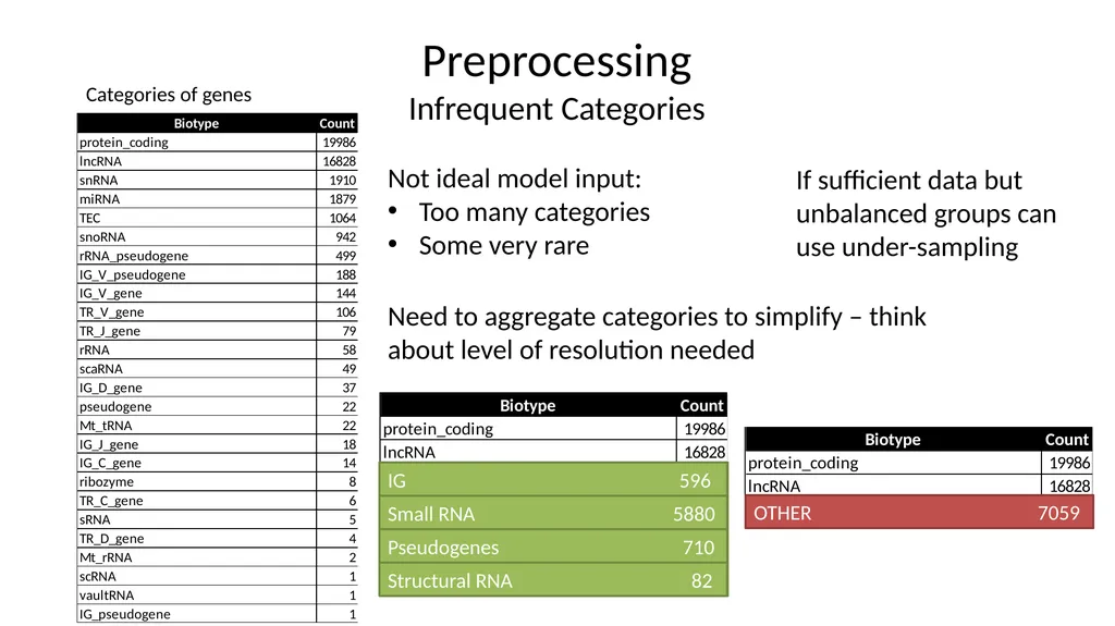
slide80. Preprocessing Infrequent Categories Categories of genes Not ideal model input:
Too many categories
Some very rare Need to aggregate categories to simplify – think about level of resolution needed If sufficient data but unbalanced groups can use under-sampling<br>
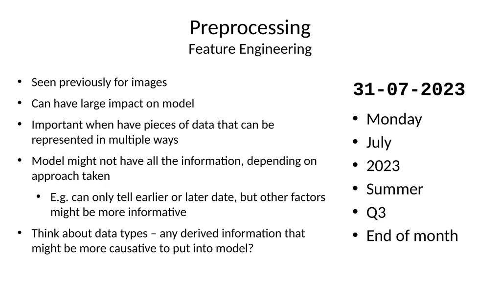
slide81. Preprocessing Feature Engineering Monday
July
2023
Summer
Q3
End of month 31-07-2023 Seen previously for images
Can have large impact on model
Important when have pieces of data that can be represented in multiple ways
Model might not have all the information, depending on approach taken
E.g. can only tell earlier or later date, but other factors might be more informative
Think about data types – any derived information that might be more causative to put into model?<br>
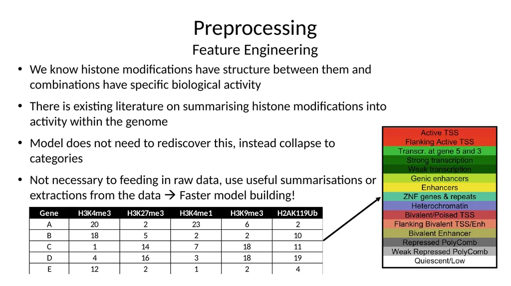
slide82. Preprocessing Feature Engineering We know histone modifications have structure between them and combinations have specific biological activity
There is existing literature on summarising histone modifications into activity within the genome
Model does not need to rediscover this, instead collapse to categories
Not necessary to feeding in raw data, use useful summarisations or extractions from the data Faster model building!<br>
slide83. Preprocessing Scaling and Normalising Some models expect numerical data which behaves in a roughly normal manner
Naïve Bayes, Linear Modelling, Neural Nets
Transformations make data more usable
Log transformation
Mean centering
Z-score normalisation
Converting to ranks
Often dealing with high-dimensional data More advanced transformations
PCA to remove noise (e.g. single cell data)<br>
slide84. Preprocessing Data Filtering Good idea to reduce the data complexity
Remove noise
Reduce size (runs quicker)
Remove variables or cases which aren't helpful
Outlier values
Poorly measured features
Redundant features, e.g. highly correlated variables
Features with no variability<br>
slide85. Practical Machine Learning using R and tidymodels<br>
slide86. Baseline R Come on an R Course! Introduction to R: https://biotrain.tv/courses/r_intro
Advanced R: https://biotrain.tv/courses/r_advanced
Plotting with GGPlot: https://biotrain.tv/courses/r_ggplot<br>
slide87. Data Analysis Workflow Raw Data Collection Preparation Formalisation Outcome<br>
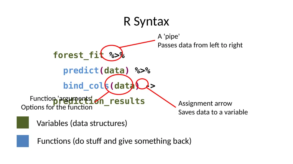
slide88. R Syntax forest_fit %>%
predict(data) %>%
bind_cols(data) -> prediction_results<br>
slide89. Packages for machine learning in R lm
nnet
rpart
brulee
kknn
ranger
h2o
mboost spark
glmnet
keras
partykit
aorsf
stan
kernlab
thief tbats
survival
xrf
hurdle
aorsf
gee
lmer
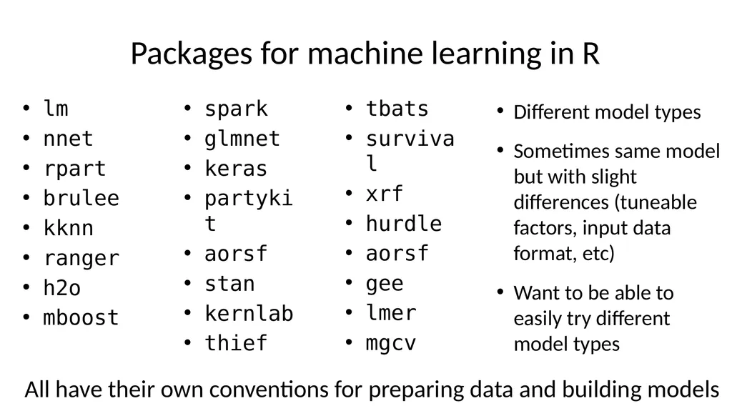
mgcv All have their own conventions for preparing data and building models<br>
slide90. Packages for machine learning in R lm
nnet
rpart
brulee
kknn
ranger
h2o
mboost spark
glmnet
keras
partykit
aorsf
stan
kernlab
thief tbats
survival
xrf
hurdle
aorsf
gee
lmer
mgcv All have their own conventions for preparing data and building models Different model types
Sometimes same model but with slight differences (tuneable factors, input data format, etc)
Want to be able to easily try different model types<br>
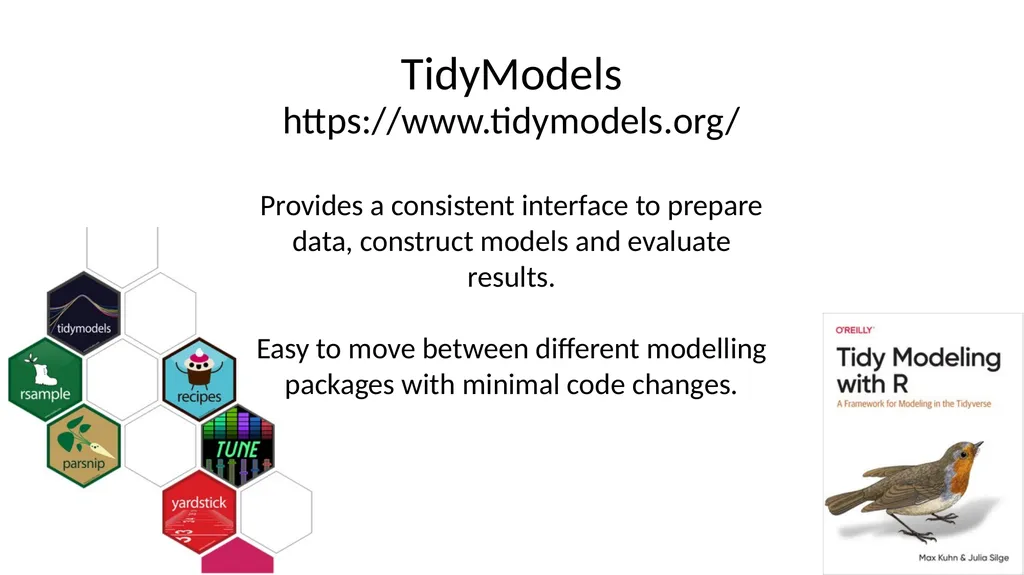
slide91. TidyModels https://www.tidymodels.org/ Provides a consistent interface to prepare data, construct models and evaluate results.
Easy to move between different modelling packages with minimal code changes.<br>
slide92. Input Data Tibble of data (2D Spreadsheet)
Read in as e.g. tsv, csv, excel spreadsheet
Rows are observations (cases) columns are variables
Classification variables must be factors (not text)
Standard exploration / plotting should happen before modelling (not covered today)<br>
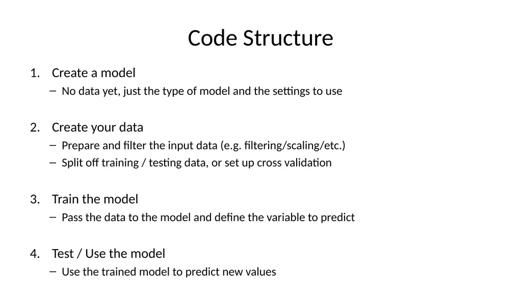
slide93. Code Structure Create a model
No data yet, just the type of model and the settings to use
Create your data
Prepare and filter the input data (e.g. filtering/scaling/etc.)
Split off training / testing data, or set up cross validation
Train the model
Pass the data to the model and define the variable to predict
Test / Use the model
Use the trained model to predict new values<br>
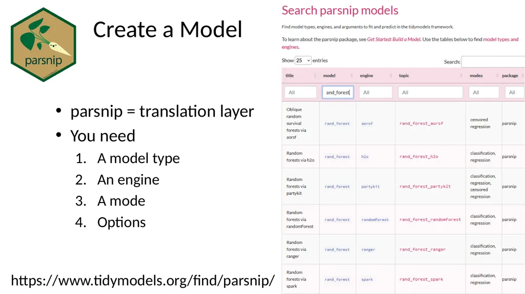
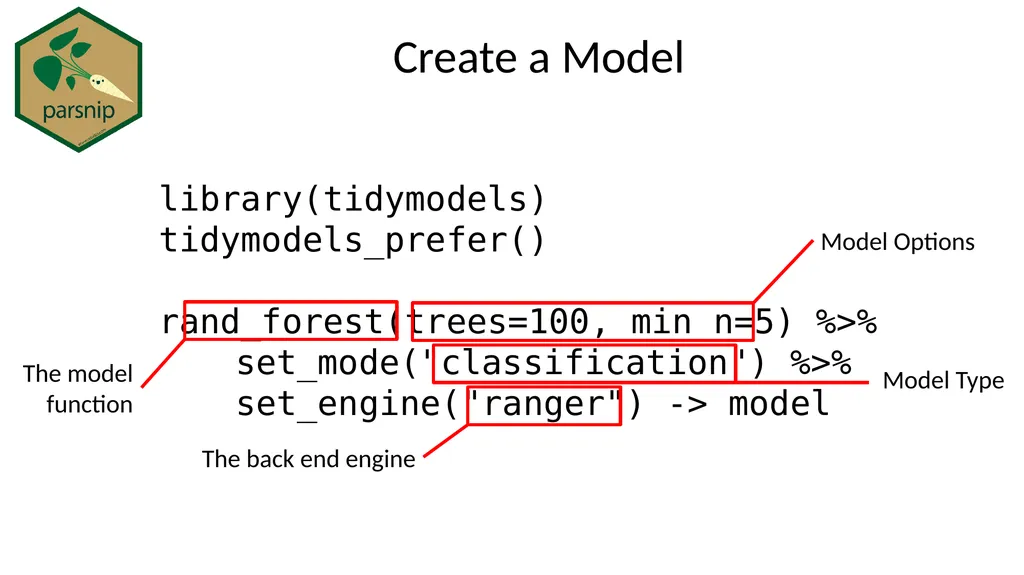
slide94. Create a Model parsnip = translation layer
You need
A model type
An engine
A mode
Options https://www.tidymodels.org/find/parsnip/<br>
slide95. Create a Model library(tidymodels)
tidymodels_prefer()
rand_forest(trees=100, min_n=5) %>%
set_mode("classification") %>%
set_engine("ranger") -> model<br>
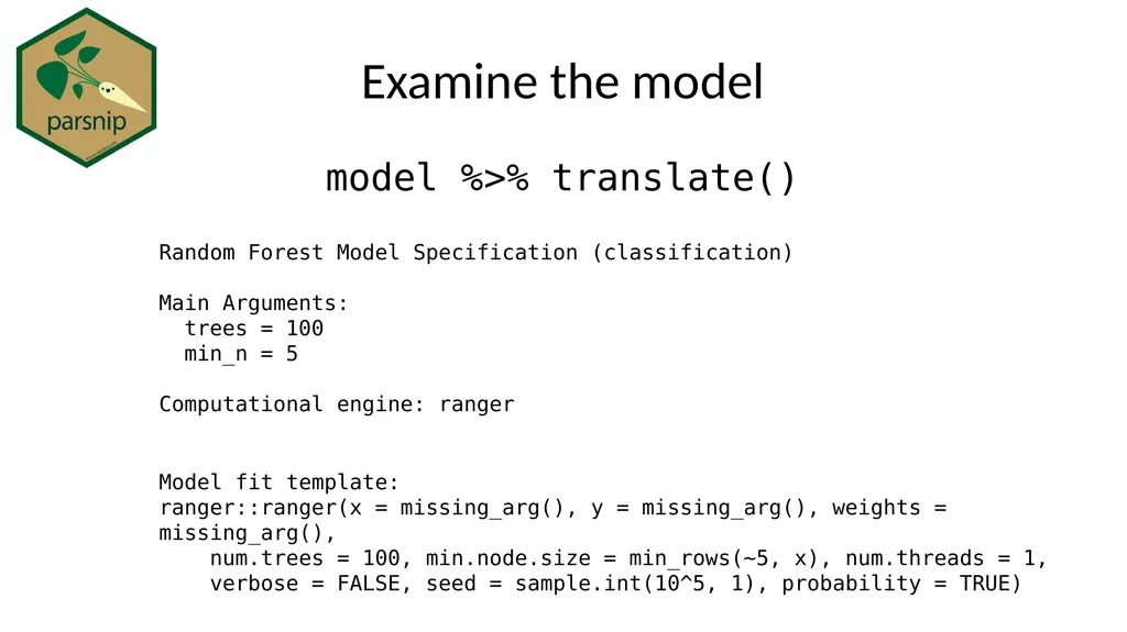
slide96. Examine the model model %>% translate() Random Forest Model Specification (classification)
Main Arguments:
trees = 100
min_n = 5
Computational engine: ranger Model fit template:
ranger::ranger(x = missing_arg(), y = missing_arg(), weights = missing_arg(),
num.trees = 100, min.node.size = min_rows(~5, x), num.threads = 1,
verbose = FALSE, seed = sample.int(10^5, 1), probability = TRUE)<br>
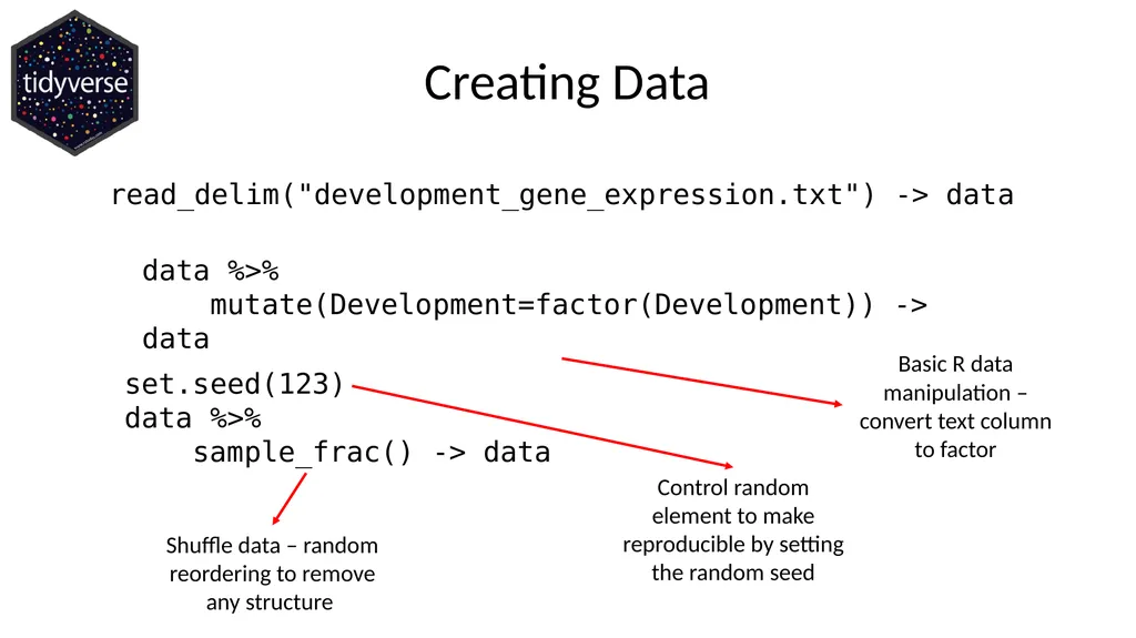
slide97. Creating Data read_delim("development_gene_expression.txt") -> data data %>%
mutate(Development=factor(Development)) -> data set.seed(123)
data %>%
sample_frac() -> data Basic R data manipulation – convert text column to factor Control random element to make reproducible by setting the random seed Shuffle data – random reordering to remove any structure<br>
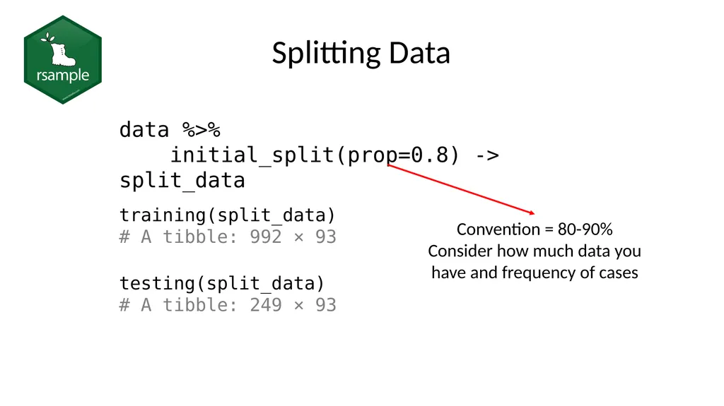
slide98. Splitting Data data %>%
initial_split(prop=0.8) -> split_data training(split_data)
# A tibble: 992 × 93 testing(split_data)
# A tibble: 249 × 93 Convention = 80-90%
Consider how much data you have and frequency of cases<br>
slide99. Splitting Data data %>%
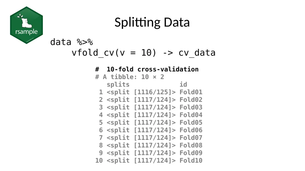
vfold_cv(v = 10) -> cv_data # 10-fold cross-validation
# A tibble: 10 × 2
splits id
1 <split [1116/125]> Fold01
2 <split [1117/124]> Fold02
3 <split [1117/124]> Fold03
4 <split [1117/124]> Fold04
5 <split [1117/124]> Fold05
6 <split [1117/124]> Fold06
7 <split [1117/124]> Fold07
8 <split [1117/124]> Fold08
9 <split [1117/124]> Fold09
10 <split [1117/124]> Fold10<br>
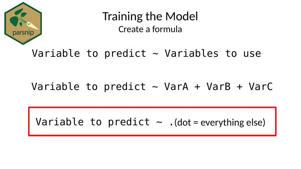
slide100. Training the Model Create a formula Variable to predict ~ Variables to use Variable to predict ~ . (dot = everything else) Variable to predict ~ VarA + VarB + VarC<br>
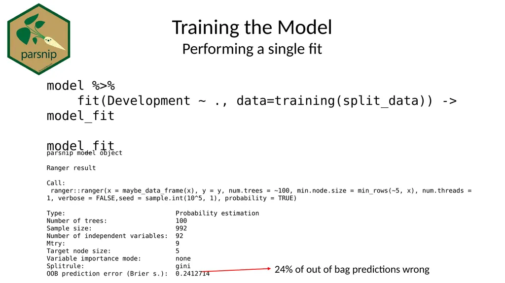
slide101. Training the Model Performing a single fit model %>%
fit(Development ~ ., data=training(split_data)) -> model_fit
model_fit parsnip model object
Ranger result
Call:
ranger::ranger(x = maybe_data_frame(x), y = y, num.trees = ~100, min.node.size = min_rows(~5, x), num.threads = 1, verbose = FALSE,seed = sample.int(10^5, 1), probability = TRUE)
Type: Probability estimation
Number of trees: 100
Sample size: 992
Number of independent variables: 92
Mtry: 9
Target node size: 5
Variable importance mode: none
Splitrule: gini
OOB prediction error (Brier s.): 0.2412714 24% of out of bag predictions wrong<br>
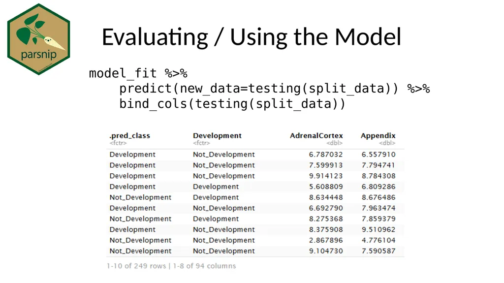
slide102. %>%
bind_cols(testing(split_data)) Evaluating / Using the Model model_fit %>%
predict(new_data=testing(split_data))<br>
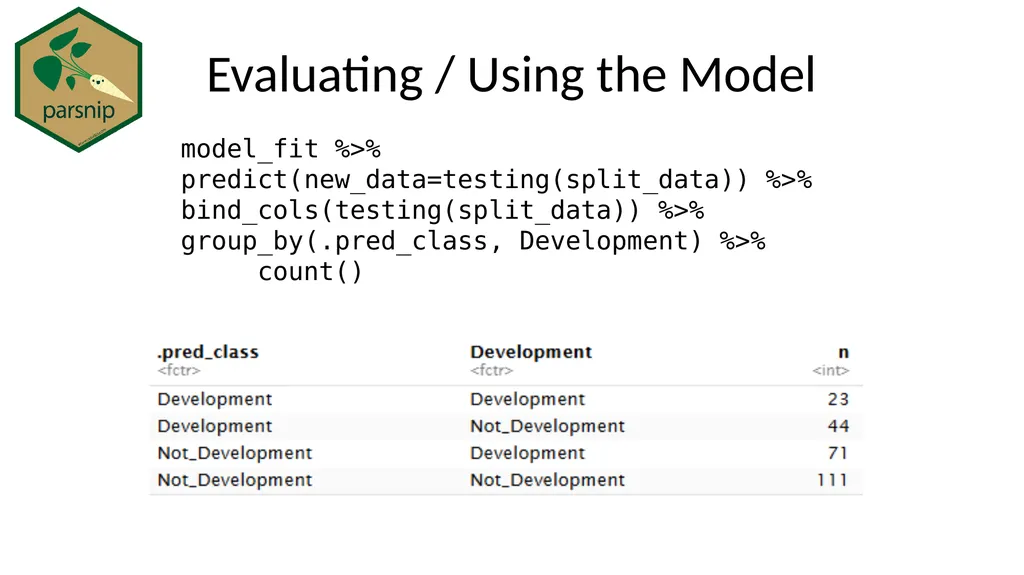
slide103. Evaluating / Using the Model model_fit %>% predict(new_data=testing(split_data)) %>% bind_cols(testing(split_data)) %>% group_by(.pred_class, Development) %>%
count()<br>
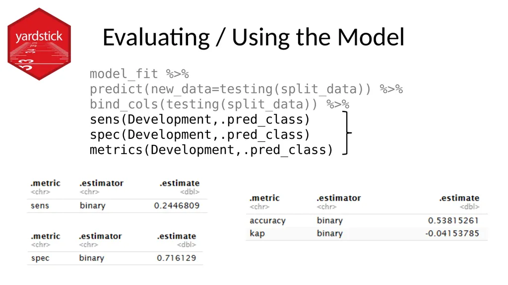
slide104. Evaluating / Using the Model model_fit %>% predict(new_data=testing(split_data)) %>% bind_cols(testing(split_data)) %>%
sens(Development,.pred_class)
spec(Development,.pred_class)
metrics(Development,.pred_class)<br>
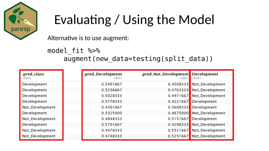
slide105. Evaluating / Using the Model Alternative is to use augment:
model_fit %>%
augment(new_data=testing(split_data))<br>
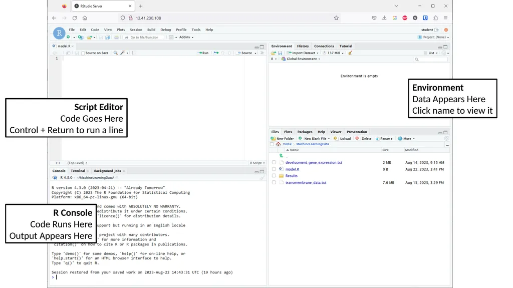
slide106. Script Editor
Code Goes Here
Control + Return to run a line R Console
Code Runs Here
Output Appears Here Environment
Data Appears Here
Click name to view it<br>
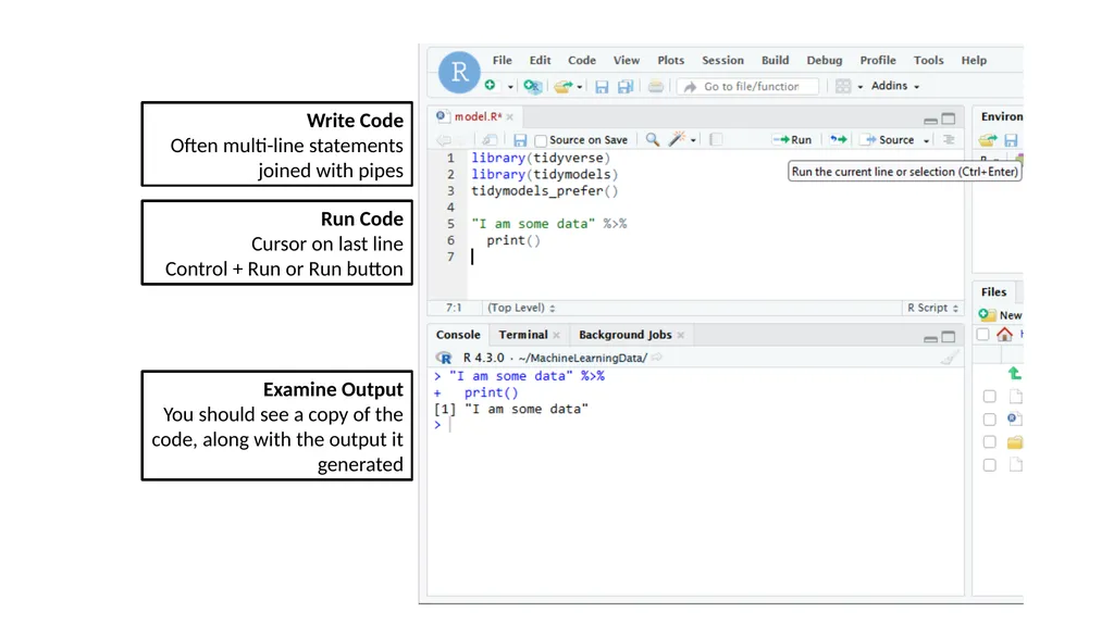
slide107. Write Code
Often multi-line statements joined with pipes Run Code
Cursor on last line
Control + Run or Run button Examine Output
You should see a copy of the code, along with the output it generated<br>
slide108. Exercise: Building a model in tidymodels<br>
slide109. Automation with Recipes and Workflows Preprocessing often has multiple steps
Need to apply these to training, testing and future data
Manually preprocessing is tedious and potentially inconsistent
Recipes let you automate this
More work initially but more reproducible
Workflows bring everything together<br>
slide110. Create a recipe
Specify formula and optionally data (shows what looks like)
Add processing steps
Filtering, Transformation etc.
Create a model
Same as we did before
Create a workflow
Combine the recipe and model together Automation with Recipes and Workflows<br>
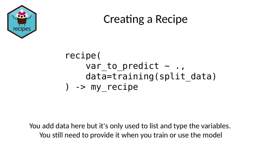
slide111. Creating a Recipe recipe(
var_to_predict ~ .,
data=training(split_data)
) -> my_recipe You add data here but it's only used to list and type the variables. You still need to provide it when you train or use the model<br>
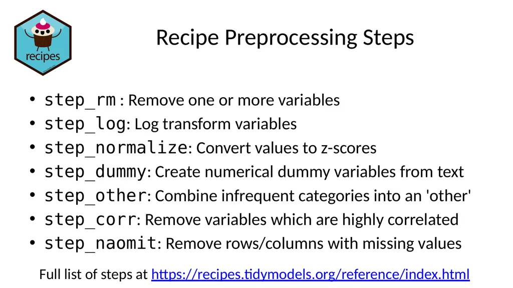
slide112. step_rm : Remove one or more variables
step_log: Log transform variables
step_normalize: Convert values to z-scores
step_dummy: Create numerical dummy variables from text
step_other: Combine infrequent categories into an 'other'
step_corr: Remove variables which are highly correlated
step_naomit: Remove rows/columns with missing values Recipe Preprocessing Steps Full list of steps at https://recipes.tidymodels.org/reference/index.html<br>
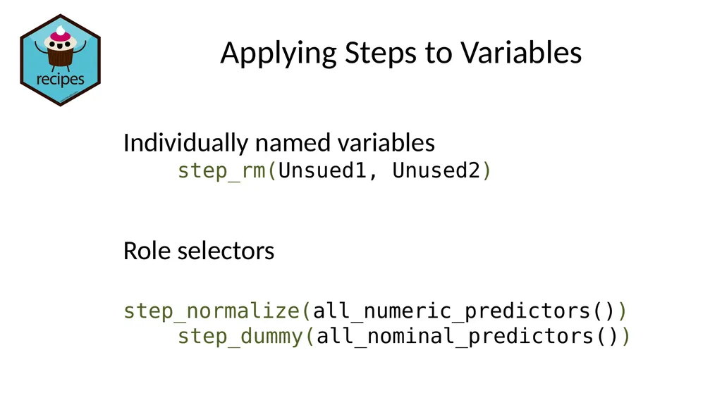
slide113. Applying Steps to Variables Individually named variables
step_rm(Unsued1, Unused2)
Role selectors
step_normalize(all_numeric_predictors())
step_dummy(all_nominal_predictors())<br>
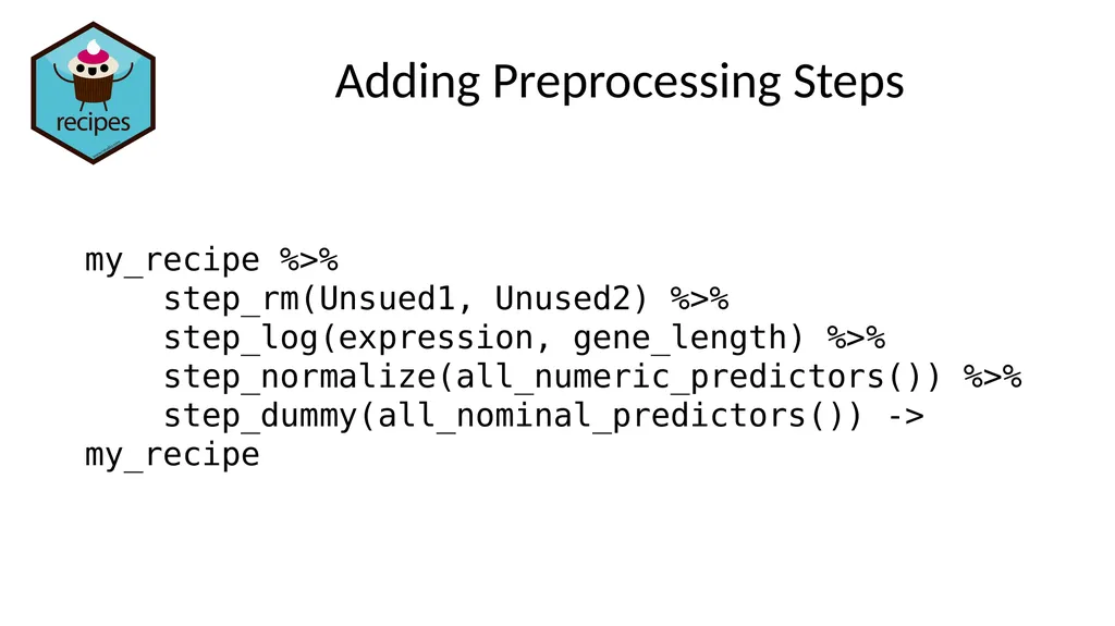
slide114. Adding Preprocessing Steps my_recipe %>%
step_rm(Unsued1, Unused2) %>%
step_log(expression, gene_length) %>%
step_normalize(all_numeric_predictors()) %>%
step_dummy(all_nominal_predictors()) -> my_recipe<br>
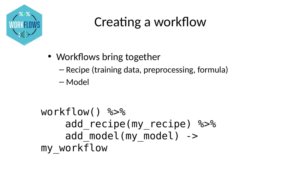
slide115. Creating a workflow Workflows bring together
Recipe (training data, preprocessing, formula)
Model workflow() %>%
add_recipe(my_recipe) %>%
add_model(my_model) -> my_workflow<br>
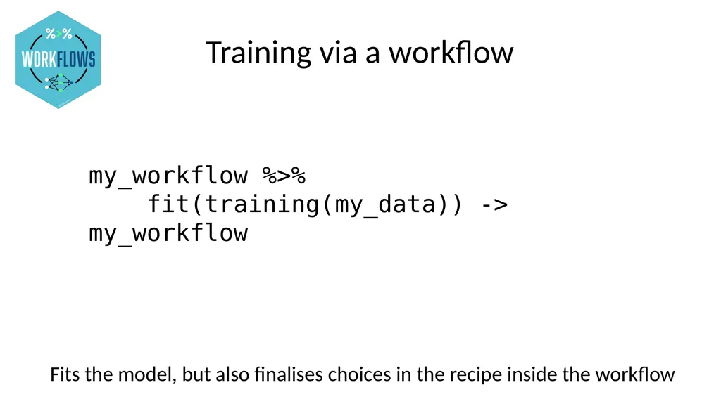
slide116. Training via a workflow my_workflow %>%
fit(training(my_data)) -> my_workflow Fits the model, but also finalises choices in the recipe inside the workflow<br>
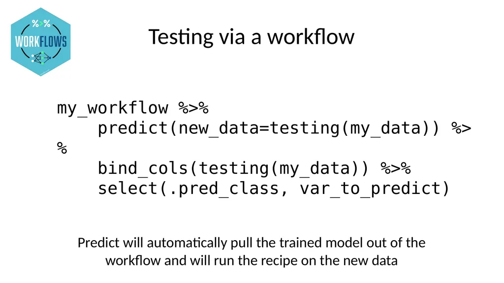
slide117. Testing via a workflow my_workflow %>%
predict(new_data=testing(my_data)) %>%
bind_cols(testing(my_data)) %>%
select(.pred_class, var_to_predict) Predict will automatically pull the trained model out of the workflow and will run the recipe on the new data<br>
slide118. Exercise: Automating models with workflows<br>
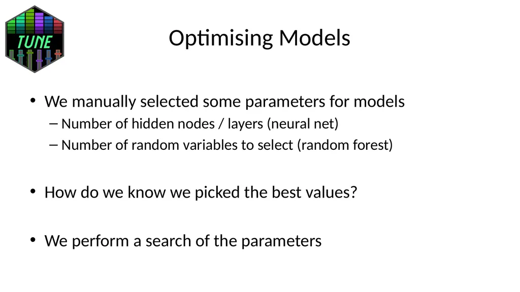
slide119. Optimising Models We manually selected some parameters for models
Number of hidden nodes / layers (neural net)
Number of random variables to select (random forest)
How do we know we picked the best values?
We perform a search of the parameters<br>
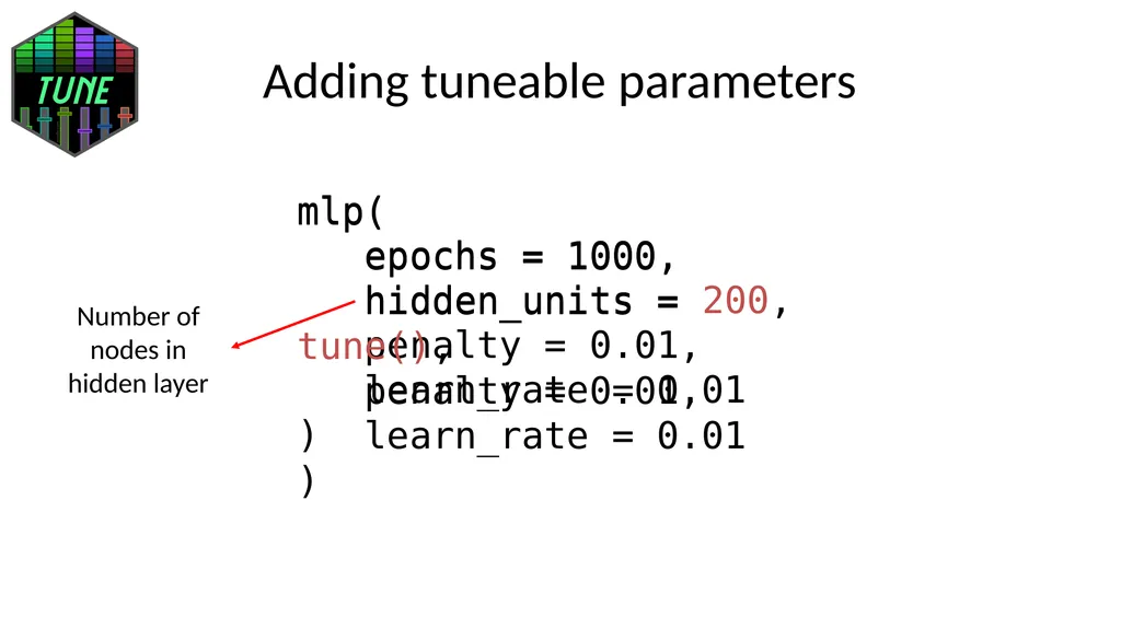
slide120. mlp(
epochs = 1000,
hidden_units = 200,
penalty = 0.01,
learn_rate = 0.01
) mlp(
epochs = 1000,
hidden_units = tune(),
penalty = 0.01,
learn_rate = 0.01
) Adding tuneable parameters Number of nodes in hidden layer<br>
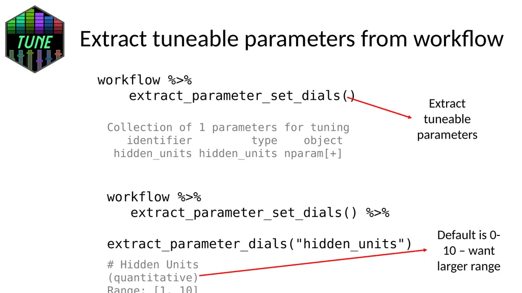
slide121. Extract tuneable parameters from workflow workflow %>%
extract_parameter_set_dials() Collection of 1 parameters for tuning
identifier type object
hidden_units hidden_units nparam[+] workflow %>%
extract_parameter_set_dials() %>%
extract_parameter_dials("hidden_units") # Hidden Units (quantitative)
Range: [1, 10] Extract tuneable parameters Default is 0-10 – want larger range<br>
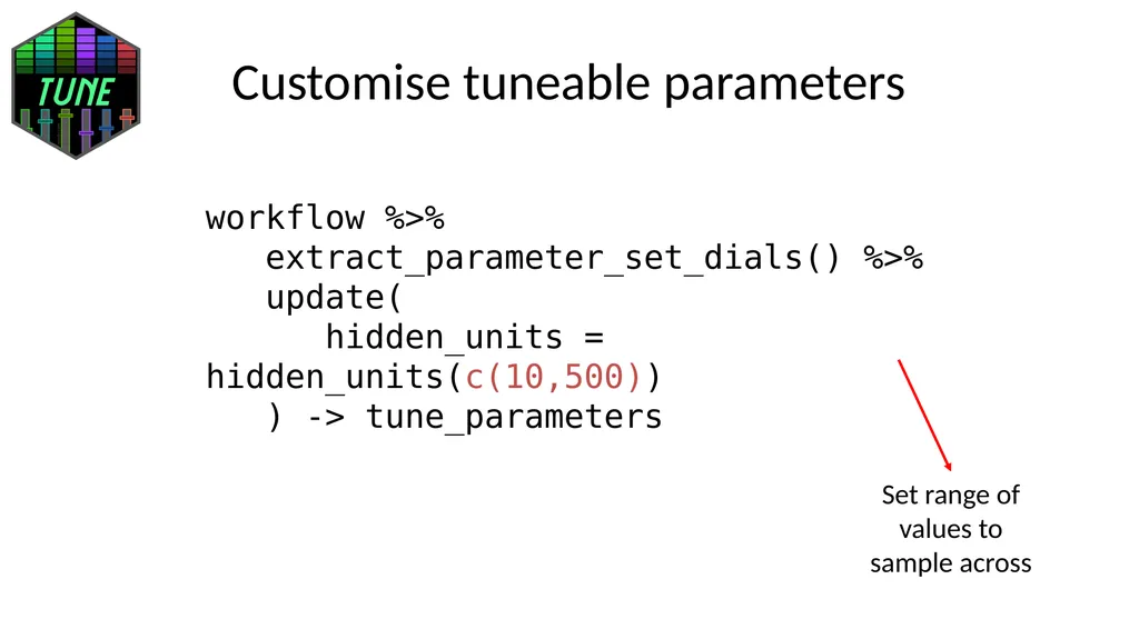
slide122. Customise tuneable parameters workflow %>%
extract_parameter_set_dials() %>%
update(
hidden_units = hidden_units(c(10,500))
) -> tune_parameters Set range of values to sample across<br>
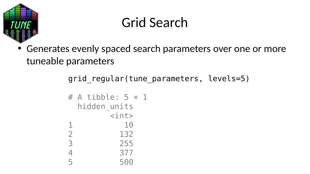
slide123. Grid Search Generates evenly spaced search parameters over one or more tuneable parameters grid_regular(tune_parameters, levels=5)
# A tibble: 5 × 1
hidden_units
<int>
1 10
2 132
3 255
4 377
5 500<br>
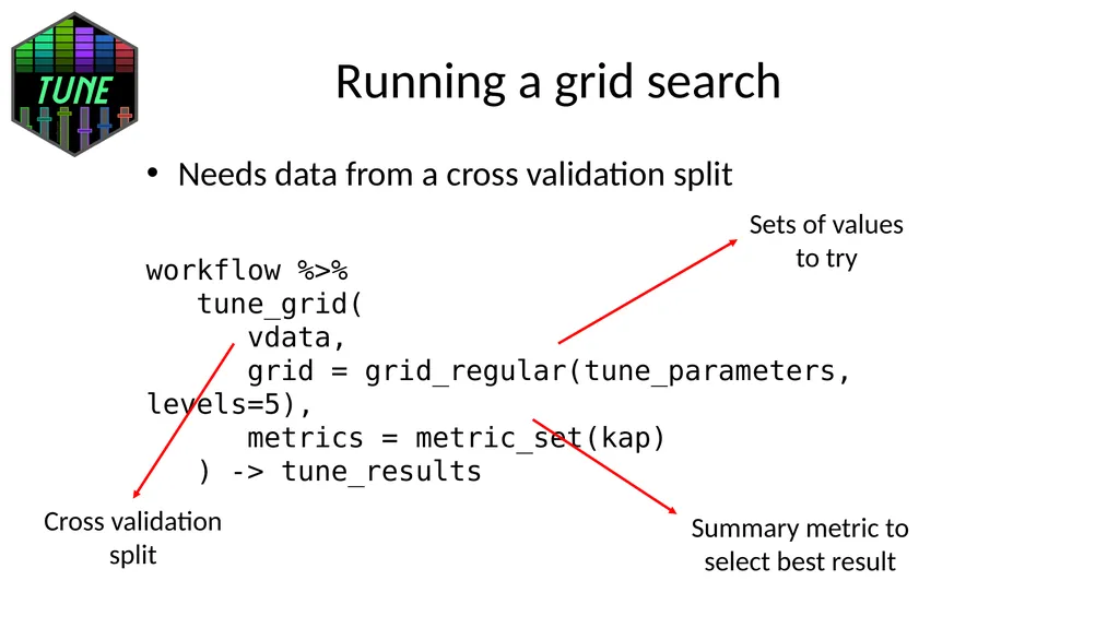
slide124. Running a grid search Needs data from a cross validation split workflow %>%
tune_grid(
vdata,
grid = grid_regular(tune_parameters, levels=5),
metrics = metric_set(kap)
) -> tune_results Sets of values to try Summary metric to select best result Cross validation split<br>
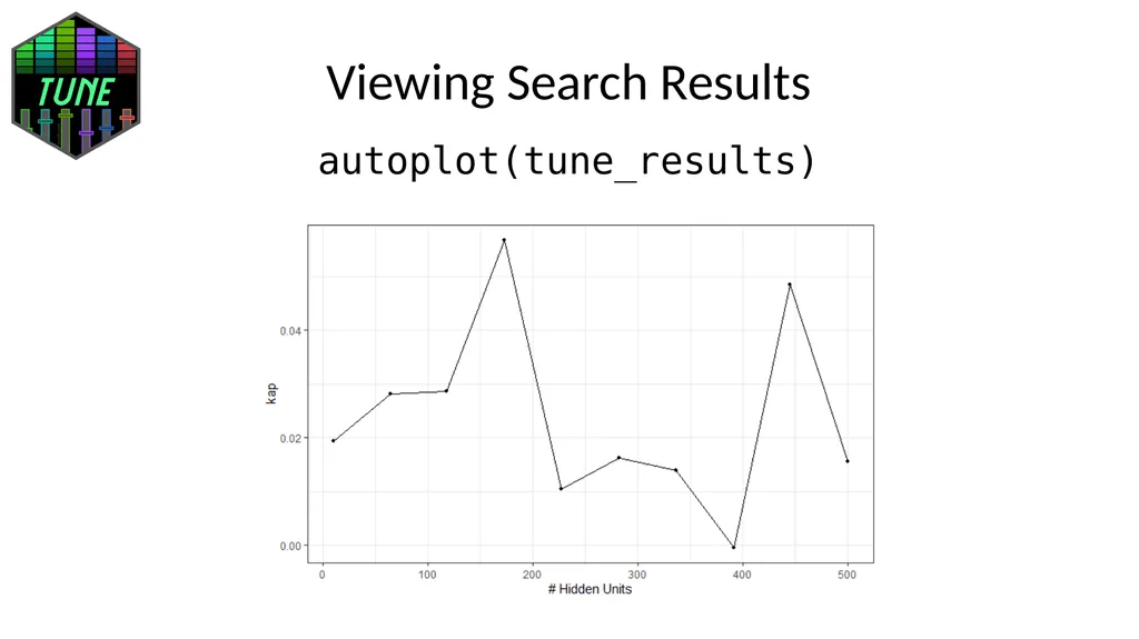
slide125. Viewing Search Results autoplot(tune_results)<br>
slide126. That’s it! - What Next? Other relevant courses?
Introduction to R (with tidyverse): 21-22nd April
Advanced R (with tidyverse): 28-29th April
Creating Complex Figures with GGPlot: 1st May
Stay in touch: contact@biotrain.tv<br>
hayley.carr@babraham.ac.uk
v2026-03<br>
slide2. Agenda for the day What is machine learning
Different types of machine learning model
[Exercise] Running different models
How to evaluate models
[Exercise] Evaluating Models
Preparing Input Data
Running Models with tidymodels
[Exercise] Building your first model
Automation with Recipes and Workflows
[Optimising models]<br>
slide3. What is Machine Learning?<br>
slide4. Data Analysis Workflow Raw Data Collection Preparation Formalisation Outcome<br>
slide5. Machine Learning Builds a Model to make Predictions<br>
slide6. Biological Examples Input: DNA Methylation from genomic CpGs
Output: Estimated biological age<br>
slide7. Biological Examples Input: DAPI stained cell images
Output: Predicted Cell Cycle Stage<br>
slide8. Biological Examples Input: Histopathology slide images
Output: Cancer likelihood score<br>
slide9. Steps in Machine Learning Generate data for samples where the outcome is known Refine the model<br>
slide10. Different machine learning models<br>
slide12. Outcome type
Regression models for quantitative predictions
Classification models for categorical predictions
Some model types can do both
Input type
Some models require all of their variables to be numeric
May need to convert categorical values to numbers
Expected behaviour of input data
Variation in the number of viable measures Differences between models<br>
slide13. K-Nearest Neighbours (KNN) models<br>
slide14. K-nearest neighbours Add a new point
Find the K (5 in this case) closest points
Count the categories in the closest points
The highest vote wins<br>
slide15. Distance Measures Quantitative:
Euclidean Distance (straight line)
Manhattan Distance (along each axis)
Categorical:
Hamming Distance (how many categories need to switch to make match)
Jaccard Distance
… Manhattan Euclidean Sample 1 Sample 2 Hamming = 2 differences<br>
slide16. Support Vector Machine (SVM) models<br>
slide17. Support Vector Machines Projects data into a multi-dimensional space
Divides the space into areas representing different categories "Hyperplane" Margin<br>
slide18. Group 2 Group 1 Clever Support Vector Machines Hyperplane positions generated after multiple runs with different subsets to optimise positions<br>
slide19. Clever Support Vector Machines<br>
slide20. Support Vector Machines Project data into higher dimensions find a support vector classifier that divides groups
Can use or define different kernel functions
Differ in how they “transform” data/how they define threshold
Previous slide = polynomial, second degree (squared values)<br>
slide21. Naïve Bayes Models<br>
slide22. Naïve Bayesian Bayes' Theorem states that the conditional probability of an event, based on the occurrence of another event, is equal to the likelihood of the second event given the first event multiplied by the probability of the first event. We calculate a set of probabilities for each variable, based on the "Disease Linked Classification"<br>
slide23. Categorical Probabilities p Chr1 | Disease = 5 / 8 = 0.625
p Chr2 | Disease = 2 / 8 = 0.250
p ChrX | Disease = 1 / 8 = 0.125 p Chr1 | Non Disease = 6 / 76 = 0.079
p Chr2 | Non Disease = 20 / 76 = 0.263
p ChrX | Non Disease = 50 / 76 = 0.658 Disease genes are more likely to be on Chr1 and Non Disease genes are more likely to be on ChrX<br>
slide24. Quantitative Probabilities State mean stdev
Disease 42.3 10.10
Non Disease 65.0 8.99 Assumption: quantitative values are normally distributed<br>
slide25. Naïve Bayes Predictions Predict the state for a new datapoint
Chromosome is 1
GC content is 40% New data is predicted to be Disease Non -<br>
slide26. Decision Trees<br>
slide27. Predict Cancer Risk with a Decision Tree Smokes? Age <50? Exercises? High<br>
slide28. How do you build a tree? From a population of observations
Which variable do you use when?
[If quantitative] which cutoff do you use?
Answer: you calculate an ‘impurity’ score and pick the least ‘impure’ variable to split the remaining data
Want to use the most cleanly predictive question to improve the tree<br>
slide29. Calculating Categorical Impurity Smoker? 30 70 Outcome is ‘impure’ because there are a mix of high and low risk individuals in each node. Node impurity = 1 – (p High)2 – (p Low)2 1 – (18/20)2 – (2/20)2
0.180 1 – (12/80)2 – (68/80)2
0.255 Weighted Average of Node Impurities = 0.18 * (20/100) + 0.255 * (80/100) = 0.24 Repeat for each question & select lowest impurity = Gini impurity Gini gain compares the weighted average of the new nodes with the impurity of the parent node 0.42-0.24 = 0.18<br>
slide30. Calculating Quantitative Impurity Take mid-point between 34 and 58<br>
slide31. Pruning Trees Lower branches may provide minimal additional information
Leaves don’t need to be completely pure
Can terminate the tree early and pick the majority answer
When to stop can be determined by node size<br>
slide32. Random Forests<br>
slide33. Random Forest Decision trees can be fragile
Prone to overfitting – too specific to training data
Deterministic – same result every time
Many trees are better than one! Bagging Bootstrapping
Selecting multiple random subsets of data<br>
slide34. Bootstrapping Two Levels of Randomisation Smoker | Exercises
Age | Exercises
Age | Smoker<br>
slide35. Build a Forest (hundreds of trees) Evaluate
Run the “out of bag” data through the trees
See how often they predict correctly
Random variable number and
number of trees can be optimised Predict
Run new data down all trees
Count the predicted outcomes
Most frequent outcome wins<br>
slide36. Feature Selection Smoker | Exercises
Age | Exercises
Age | Smoker Smoker | Exercises
Age | Exercises
Age | Smoker More informative features will appear higher up the tree.
Can aggregate this information across the forest<br>
slide37. Neural Networks<br>
slide38. Neural Network Structure Input Node Layer<br>
slide39. Neural Network Structure Input Hidden Output<br>
slide40. Neural Network Structure Input Hidden Output<br>
slide41. Using the network Hidden Output Input<br>
slide42. Neural Networks 0.1 0.9 0.5 Node Layer 0.6 0.2 0.9 Activation Value<br>
slide43. Calculating Node Values 0.1 0.9 0.5 ? +0.5 +3.1 -1.9 Weight (0.1 x 0.5) + (0.9 x 3.1) + (0.5 x -1.9) = 1.89 Sigmoid output = 0.87 Sigmoid output (bias 2) = 0.47 Training = Calculating Weights and Biases and optimising ∑(activation x weight)<br>
slide44. Neural Network Structure Input Hidden Output<br>
slide45. Training the network Selecting the number of hidden layers Number of layers changes the type of relationships modelled
0 hidden layers = linear relationship, similar to linear modelling
1 hidden layer = nonlinear relationships
2 hidden layers = nonlinear relationships with arbitrary boundaries Most problems only require 1 hidden layer. More complex data can benefit from 2. Virtually nothing requires more than two.<br>
slide46. Training the network Selecting the number of nodes in hidden layers Too few nodes will not allow enough complexity to model the system effectively
Too many nodes will overfit – essentially "memorising" the training data Number of hidden layer nodes should be between the input number and the output number Simple
Try 2/3 input number plus output number Complex
Nh = number of hidden nodes
Ni = number of input nodes
No = number of output nodes
Ns = size of training set
α = scaling factor (normally 2) Gives starting point, then can optimise<br>
slide47. Training the network Selecting weights and biases Generate a "cost function" – a numerical value which says how well the model performed on the training data (high = bad, low = good)
Could just be how good the predictions are, but often good to include how complex the connections are<br>
slide48. Training the network Back Propagation How do you increase a value?
Increase positive weights
Tied to high activations upstream
Decrease negative weights
Tied to high activations upstream
What doesn't matter?
Anything with a low weight
Anything with a low upstream activation Disease No Disease Prediction for a single disease sample
Average across all samples and then adjust Should be lower 0.6 0.7<br>
slide49. Cleaning the network Good idea to minimise the network
Remove nodes where all output weights are low
Having little effect on the rest of the network<br>
slide50. Exercise: Trying different models<br>
slide51. Exercise 1: summary points Part 1:
Some models are deterministic, some are not
Some are variable when run multiple times, some are different but fairly stable
Just because more complex, doesn’t mean a better model
More complex also means more running time!
Part 2:
Multiple parameters that can be changed, involved building lots of different models
Trade off between optimisation and time<br>
slide52. Evaluating Models<br>
slide53. A good model?<br>
slide54. Baseline for comparison 1000 patients, 10 have disease
Assign most common category (healthy) to everyone
990 correct = 99% success!
A good model must do better than this.<br>
slide55. Evaluating Qualitative Models Rather than overall success rate, break down by category Confusion matrix<br>
slide56. Evaluating Qualitative Models (88+24) = 112 correct
(4+6) = 10 incorrect
Overall = 92% correct (88+4) = 92 correct
(4+1) = 5 incorrect
Overall = 95% correct (78+28) = 106 correct
(0+16) = 16 incorrect
Overall = 91% correct<br>
slide57. Sensitivity vs Specificity Overall = 92% correct
Sensitivity = 24/28 = 86%
Specificity = 88/94 = 94% Sensitivity: How likely is the model to identify diseased patients correctly
Specificity: How likely is the model to identify healthy patients correctly Overall = 95% correct
Sensitivity = 4/8 = 50%
Specificity = 88/89 = 99% Overall = 91% correct
Sensitivity = 28/28 = 100%
Specificity = 78/94 = 83%<br>
slide58. Sensitivity vs Specificity What matters more? Overall = 92% correct
Sensitivity = 24/28 = 86%
Specificity = 88/94 = 94% Overall = 95% correct
Sensitivity = 4/8 = 50%
Specificity = 88/89 = 99% Overall = 91% correct
Sensitivity = 28/28 = 100%
Specificity = 78/94 = 83% Getting both is ideal – obviously!
If never missing disease is the main concern favour sensitivity
If not incorrectly false predictions is important favour specificity
Need to consider the frequency of true positives<br>
slide59. Cohen's Kappa Score Measures whether the predictions are correct more often that you'd expect if the model was just guessing
Takes into account the proportion of predictions and observations in each class<br>
slide60. Area Under the ROC Curve (AUC) ROC curves plot the model’s True Positive Rate (TPR) as a function of its False Positive Rate (FPR)
AUROC values of:
1.0 = a perfect classifier
0.5 = a classifier with random guessing performance
0 = the worst possible classifier
If not binary classifier then can be calculated for each class in turn and take a weighted average (e.g. by number of instances in each class) By cmglee, MartinThoma - Roc-draft-xkcd-style.svg, CC BY-SA 4.0, https://commons.wikimedia.org/w/index.php?curid=109730045<br>
slide61. Evaluating Quantitative Models Correlation/association between predictions and true values (R or R2)
How close are the predictions to the true values?
Doesn’t matter if the mistake is high or low
Need a single value to summarise the total error<br>
slide62. Evaluating Quantitative Models Line of perfect fit Square differences (all positive)
Sum differences = single value
Sum of Squared Differences
SSD<br>
slide63. Exercise: Evaluating Models<br>
slide64. Making best use of your data when building and testing models<br>
slide65. Data is Precious<br>
slide66. Overfitting Rules are too specific
Works brilliantly on the training data
Won't work well on new data Has my model learned useful trends from the data, or just 'memorised' the training data? Model:
If weight is >=28 or weight <=19 Sex is FEMALE
Otherwise Sex is MALE You can't evaluate a model using the same data used to train it<br>
slide67. Data is Precious Random Splitting<br>
slide68. Weighted Training Selection All disease samples are in the testing set
Nothing left to train on.
Biased selection maintains a balance of outcomes in each group<br>
slide69. Performance could depend on data split 90% Accurate Model 80% Accurate Model<br>
slide70. Cross Validation<br>
slide71. Cross Validation<br>
slide72. 10-Fold Cross Validation<br>
slide73. Input Data<br>
slide74. Garbage in = Garbage out Data Cleaning, Filtering, Scaling and Feature Construction<br>
slide75. Common Data Problems Data Leakage Accidentally including something unintentional which reveals the true prediction for the case Audio clips from right whales were shorter than those from other species.
The right whale clips were next to each other in the dataset Healthy scans came from children
COVID scans came from people lying down
Models recognised the font on the scan pictures<br>
slide76. Common Data Problems Outliers
Extreme values, or just mistakes, will skew summary metrics
Missing values
Handled poorly by many models, either remove, or impute (with care)
Noisy variables
Variables with no connection to the question. Slow modelling and make results worse
Different scales
Quantitative models benefit from having variables with similar ranges of values<br>
slide77. Preprocessing Converting to Numbers Some models require all data to be numeric
Linear Models, SVM, Neural Nets
Create ‘dummy variables’
Some don’t care
Decision trees, Random Forest<br>
slide78. Pre-processing Some models cannot use categorical data as input – create a dummy variable
Converted original sequence data to digital matrix for SVM model input:
‘A’ = [1, 0, 0, 0]; ‘G’ = [0, 1, 0, 0]; ‘C’ = [0, 0, 1, 0]; ‘T’ = [0, 0, 0, 1]
E.g. ‘AGT’ becomes [1, 0, 0, 0, 0, 1, 0, 0, 0, 0, 0, 1]
Can alternatively have a ‘baseline’ value, e.g.:
A = [0, 0 ,0]; G = [1, 0, 0]; C = [0, 1, 0]; T = [0, 0, 1] One-hot encoding<br>
slide79. Preprocessing Converting to Numbers Stored as intensity values for RGB in each pixel Neural net input needs a linear set of values This does not scale well – too many input nodes Instead, use pre-processing to extract features or patterns within the data to use as input
reduces scale and noise<br>
slide80. Preprocessing Infrequent Categories Categories of genes Not ideal model input:
Too many categories
Some very rare Need to aggregate categories to simplify – think about level of resolution needed If sufficient data but unbalanced groups can use under-sampling<br>
slide81. Preprocessing Feature Engineering Monday
July
2023
Summer
Q3
End of month 31-07-2023 Seen previously for images
Can have large impact on model
Important when have pieces of data that can be represented in multiple ways
Model might not have all the information, depending on approach taken
E.g. can only tell earlier or later date, but other factors might be more informative
Think about data types – any derived information that might be more causative to put into model?<br>
slide82. Preprocessing Feature Engineering We know histone modifications have structure between them and combinations have specific biological activity
There is existing literature on summarising histone modifications into activity within the genome
Model does not need to rediscover this, instead collapse to categories
Not necessary to feeding in raw data, use useful summarisations or extractions from the data Faster model building!<br>
slide83. Preprocessing Scaling and Normalising Some models expect numerical data which behaves in a roughly normal manner
Naïve Bayes, Linear Modelling, Neural Nets
Transformations make data more usable
Log transformation
Mean centering
Z-score normalisation
Converting to ranks
Often dealing with high-dimensional data More advanced transformations
PCA to remove noise (e.g. single cell data)<br>
slide84. Preprocessing Data Filtering Good idea to reduce the data complexity
Remove noise
Reduce size (runs quicker)
Remove variables or cases which aren't helpful
Outlier values
Poorly measured features
Redundant features, e.g. highly correlated variables
Features with no variability<br>
slide85. Practical Machine Learning using R and tidymodels<br>
slide86. Baseline R Come on an R Course! Introduction to R: https://biotrain.tv/courses/r_intro
Advanced R: https://biotrain.tv/courses/r_advanced
Plotting with GGPlot: https://biotrain.tv/courses/r_ggplot<br>
slide87. Data Analysis Workflow Raw Data Collection Preparation Formalisation Outcome<br>
slide88. R Syntax forest_fit %>%
predict(data) %>%
bind_cols(data) -> prediction_results<br>
slide89. Packages for machine learning in R lm
nnet
rpart
brulee
kknn
ranger
h2o
mboost spark
glmnet
keras
partykit
aorsf
stan
kernlab
thief tbats
survival
xrf
hurdle
aorsf
gee
lmer
mgcv All have their own conventions for preparing data and building models<br>
slide90. Packages for machine learning in R lm
nnet
rpart
brulee
kknn
ranger
h2o
mboost spark
glmnet
keras
partykit
aorsf
stan
kernlab
thief tbats
survival
xrf
hurdle
aorsf
gee
lmer
mgcv All have their own conventions for preparing data and building models Different model types
Sometimes same model but with slight differences (tuneable factors, input data format, etc)
Want to be able to easily try different model types<br>
slide91. TidyModels https://www.tidymodels.org/ Provides a consistent interface to prepare data, construct models and evaluate results.
Easy to move between different modelling packages with minimal code changes.<br>
slide92. Input Data Tibble of data (2D Spreadsheet)
Read in as e.g. tsv, csv, excel spreadsheet
Rows are observations (cases) columns are variables
Classification variables must be factors (not text)
Standard exploration / plotting should happen before modelling (not covered today)<br>
slide93. Code Structure Create a model
No data yet, just the type of model and the settings to use
Create your data
Prepare and filter the input data (e.g. filtering/scaling/etc.)
Split off training / testing data, or set up cross validation
Train the model
Pass the data to the model and define the variable to predict
Test / Use the model
Use the trained model to predict new values<br>
slide94. Create a Model parsnip = translation layer
You need
A model type
An engine
A mode
Options https://www.tidymodels.org/find/parsnip/<br>
slide95. Create a Model library(tidymodels)
tidymodels_prefer()
rand_forest(trees=100, min_n=5) %>%
set_mode("classification") %>%
set_engine("ranger") -> model<br>
slide96. Examine the model model %>% translate() Random Forest Model Specification (classification)
Main Arguments:
trees = 100
min_n = 5
Computational engine: ranger Model fit template:
ranger::ranger(x = missing_arg(), y = missing_arg(), weights = missing_arg(),
num.trees = 100, min.node.size = min_rows(~5, x), num.threads = 1,
verbose = FALSE, seed = sample.int(10^5, 1), probability = TRUE)<br>
slide97. Creating Data read_delim("development_gene_expression.txt") -> data data %>%
mutate(Development=factor(Development)) -> data set.seed(123)
data %>%
sample_frac() -> data Basic R data manipulation – convert text column to factor Control random element to make reproducible by setting the random seed Shuffle data – random reordering to remove any structure<br>
slide98. Splitting Data data %>%
initial_split(prop=0.8) -> split_data training(split_data)
# A tibble: 992 × 93 testing(split_data)
# A tibble: 249 × 93 Convention = 80-90%
Consider how much data you have and frequency of cases<br>
slide99. Splitting Data data %>%
vfold_cv(v = 10) -> cv_data # 10-fold cross-validation
# A tibble: 10 × 2
splits id
1 <split [1116/125]> Fold01
2 <split [1117/124]> Fold02
3 <split [1117/124]> Fold03
4 <split [1117/124]> Fold04
5 <split [1117/124]> Fold05
6 <split [1117/124]> Fold06
7 <split [1117/124]> Fold07
8 <split [1117/124]> Fold08
9 <split [1117/124]> Fold09
10 <split [1117/124]> Fold10<br>
slide100. Training the Model Create a formula Variable to predict ~ Variables to use Variable to predict ~ . (dot = everything else) Variable to predict ~ VarA + VarB + VarC<br>
slide101. Training the Model Performing a single fit model %>%
fit(Development ~ ., data=training(split_data)) -> model_fit
model_fit parsnip model object
Ranger result
Call:
ranger::ranger(x = maybe_data_frame(x), y = y, num.trees = ~100, min.node.size = min_rows(~5, x), num.threads = 1, verbose = FALSE,seed = sample.int(10^5, 1), probability = TRUE)
Type: Probability estimation
Number of trees: 100
Sample size: 992
Number of independent variables: 92
Mtry: 9
Target node size: 5
Variable importance mode: none
Splitrule: gini
OOB prediction error (Brier s.): 0.2412714 24% of out of bag predictions wrong<br>
slide102. %>%
bind_cols(testing(split_data)) Evaluating / Using the Model model_fit %>%
predict(new_data=testing(split_data))<br>
slide103. Evaluating / Using the Model model_fit %>% predict(new_data=testing(split_data)) %>% bind_cols(testing(split_data)) %>% group_by(.pred_class, Development) %>%
count()<br>
slide104. Evaluating / Using the Model model_fit %>% predict(new_data=testing(split_data)) %>% bind_cols(testing(split_data)) %>%
sens(Development,.pred_class)
spec(Development,.pred_class)
metrics(Development,.pred_class)<br>
slide105. Evaluating / Using the Model Alternative is to use augment:
model_fit %>%
augment(new_data=testing(split_data))<br>
slide106. Script Editor
Code Goes Here
Control + Return to run a line R Console
Code Runs Here
Output Appears Here Environment
Data Appears Here
Click name to view it<br>
slide107. Write Code
Often multi-line statements joined with pipes Run Code
Cursor on last line
Control + Run or Run button Examine Output
You should see a copy of the code, along with the output it generated<br>
slide108. Exercise: Building a model in tidymodels<br>
slide109. Automation with Recipes and Workflows Preprocessing often has multiple steps
Need to apply these to training, testing and future data
Manually preprocessing is tedious and potentially inconsistent
Recipes let you automate this
More work initially but more reproducible
Workflows bring everything together<br>
slide110. Create a recipe
Specify formula and optionally data (shows what looks like)
Add processing steps
Filtering, Transformation etc.
Create a model
Same as we did before
Create a workflow
Combine the recipe and model together Automation with Recipes and Workflows<br>
slide111. Creating a Recipe recipe(
var_to_predict ~ .,
data=training(split_data)
) -> my_recipe You add data here but it's only used to list and type the variables. You still need to provide it when you train or use the model<br>
slide112. step_rm : Remove one or more variables
step_log: Log transform variables
step_normalize: Convert values to z-scores
step_dummy: Create numerical dummy variables from text
step_other: Combine infrequent categories into an 'other'
step_corr: Remove variables which are highly correlated
step_naomit: Remove rows/columns with missing values Recipe Preprocessing Steps Full list of steps at https://recipes.tidymodels.org/reference/index.html<br>
slide113. Applying Steps to Variables Individually named variables
step_rm(Unsued1, Unused2)
Role selectors
step_normalize(all_numeric_predictors())
step_dummy(all_nominal_predictors())<br>
slide114. Adding Preprocessing Steps my_recipe %>%
step_rm(Unsued1, Unused2) %>%
step_log(expression, gene_length) %>%
step_normalize(all_numeric_predictors()) %>%
step_dummy(all_nominal_predictors()) -> my_recipe<br>
slide115. Creating a workflow Workflows bring together
Recipe (training data, preprocessing, formula)
Model workflow() %>%
add_recipe(my_recipe) %>%
add_model(my_model) -> my_workflow<br>
slide116. Training via a workflow my_workflow %>%
fit(training(my_data)) -> my_workflow Fits the model, but also finalises choices in the recipe inside the workflow<br>
slide117. Testing via a workflow my_workflow %>%
predict(new_data=testing(my_data)) %>%
bind_cols(testing(my_data)) %>%
select(.pred_class, var_to_predict) Predict will automatically pull the trained model out of the workflow and will run the recipe on the new data<br>
slide118. Exercise: Automating models with workflows<br>
slide119. Optimising Models We manually selected some parameters for models
Number of hidden nodes / layers (neural net)
Number of random variables to select (random forest)
How do we know we picked the best values?
We perform a search of the parameters<br>
slide120. mlp(
epochs = 1000,
hidden_units = 200,
penalty = 0.01,
learn_rate = 0.01
) mlp(
epochs = 1000,
hidden_units = tune(),
penalty = 0.01,
learn_rate = 0.01
) Adding tuneable parameters Number of nodes in hidden layer<br>
slide121. Extract tuneable parameters from workflow workflow %>%
extract_parameter_set_dials() Collection of 1 parameters for tuning
identifier type object
hidden_units hidden_units nparam[+] workflow %>%
extract_parameter_set_dials() %>%
extract_parameter_dials("hidden_units") # Hidden Units (quantitative)
Range: [1, 10] Extract tuneable parameters Default is 0-10 – want larger range<br>
slide122. Customise tuneable parameters workflow %>%
extract_parameter_set_dials() %>%
update(
hidden_units = hidden_units(c(10,500))
) -> tune_parameters Set range of values to sample across<br>
slide123. Grid Search Generates evenly spaced search parameters over one or more tuneable parameters grid_regular(tune_parameters, levels=5)
# A tibble: 5 × 1
hidden_units
<int>
1 10
2 132
3 255
4 377
5 500<br>
slide124. Running a grid search Needs data from a cross validation split workflow %>%
tune_grid(
vdata,
grid = grid_regular(tune_parameters, levels=5),
metrics = metric_set(kap)
) -> tune_results Sets of values to try Summary metric to select best result Cross validation split<br>
slide125. Viewing Search Results autoplot(tune_results)<br>
slide126. That’s it! - What Next? Other relevant courses?
Introduction to R (with tidyverse): 21-22nd April
Advanced R (with tidyverse): 28-29th April
Creating Complex Figures with GGPlot: 1st May
Stay in touch: contact@biotrain.tv<br>