Introduction to Management Science Thirteenth

conchita-marotz

Published 2026-09-28 · 41 slides · 0 views

↓ Download

Introduction to Management Science Thirteenth

Introduction to Management Science Thirteenth - slide 1 of 41

Introduction to Management Science Thirteenth - slide 2 of 41

Introduction to Management Science Thirteenth - slide 3 of 41

Introduction to Management Science Thirteenth - slide 4 of 41

Introduction to Management Science Thirteenth - slide 5 of 41

Introduction to Management Science Thirteenth - slide 6 of 41

Introduction to Management Science Thirteenth - slide 7 of 41

Introduction to Management Science Thirteenth - slide 8 of 41

Introduction to Management Science Thirteenth - slide 9 of 41

Introduction to Management Science Thirteenth - slide 10 of 41

Introduction to Management Science Thirteenth - slide 11 of 41

Introduction to Management Science Thirteenth - slide 12 of 41

Introduction to Management Science Thirteenth - slide 13 of 41

Introduction to Management Science Thirteenth - slide 14 of 41

Introduction to Management Science Thirteenth - slide 15 of 41

Introduction to Management Science Thirteenth - slide 16 of 41

Introduction to Management Science Thirteenth - slide 17 of 41

Introduction to Management Science Thirteenth - slide 18 of 41

Introduction to Management Science Thirteenth - slide 19 of 41

Introduction to Management Science Thirteenth - slide 20 of 41

Introduction to Management Science Thirteenth - slide 21 of 41

Introduction to Management Science Thirteenth - slide 22 of 41

Introduction to Management Science Thirteenth - slide 23 of 41

Introduction to Management Science Thirteenth - slide 24 of 41

Introduction to Management Science Thirteenth - slide 25 of 41

Introduction to Management Science Thirteenth - slide 26 of 41

Introduction to Management Science Thirteenth - slide 27 of 41

Introduction to Management Science Thirteenth - slide 28 of 41

Introduction to Management Science Thirteenth - slide 29 of 41

Introduction to Management Science Thirteenth - slide 30 of 41

Introduction to Management Science Thirteenth - slide 31 of 41

Introduction to Management Science Thirteenth - slide 32 of 41

Introduction to Management Science Thirteenth - slide 33 of 41

Introduction to Management Science Thirteenth - slide 34 of 41

Introduction to Management Science Thirteenth - slide 35 of 41

Introduction to Management Science Thirteenth - slide 36 of 41

Introduction to Management Science Thirteenth - slide 37 of 41

Introduction to Management Science Thirteenth - slide 38 of 41

Introduction to Management Science Thirteenth - slide 39 of 41

Introduction to Management Science Thirteenth - slide 40 of 41

Introduction to Management Science Thirteenth - slide 41 of 41

Description

Introduction to Management Science Thirteenth Edition, Global Edition Chapter 3 Linear Programming: Computer Solution and Sensitivity Analysis Copyright 2019 Pearson Education, Ltd. All Rights Reserved Learning Objectives 3.1 Computer

Download this presentation From Below

"Introduction to Management Science Thirteenth" is the property of its rightful owner. Permission is granted to download and print the materials on this website for personal, non-commercial use only, and to display it on your personal computer provided you do not modify the materials and that you retain all copyright notices contained in the materials. By downloading content from our website, you accept the terms of this agreement.

Presentation Transcript

Introduction to Management Science Thirteenth Edition, Global Edition Chapter 3 Linear Programming: Computer Solution and Sensitivity Analysis Copyright © 2019 Pearson Education, Ltd. All Rights Reserved

Learning Objectives 3.1 Computer Solution
3.2 Sensitivity Analysis

Learning Objective 3.1 Computer Solution

Computer Solution Early linear programming used lengthy manual mathematical solution procedure called the Simplex Method (See web site Module A).
Steps of the Simplex Method have been programmed in software packages designed for linear programming problems.
Many such packages available currently.
Used extensively in business and government.
Text focuses on Excel Spreadsheets and Q M for Windows.

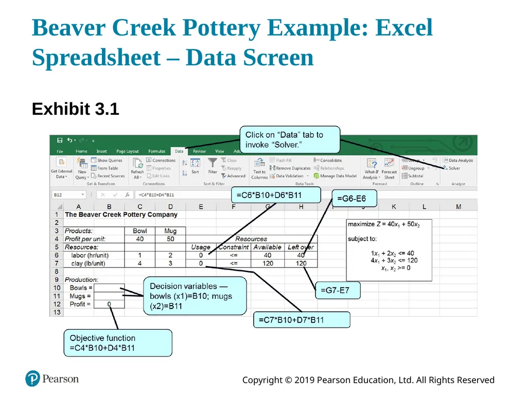
Beaver Creek Pottery Example: Excel Spreadsheet – Data Screen Exhibit 3.1

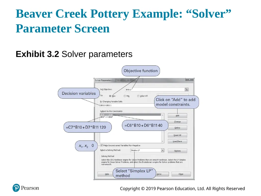
Beaver Creek Pottery Example: “Solver” Parameter Screen Exhibit 3.2 Solver parameters

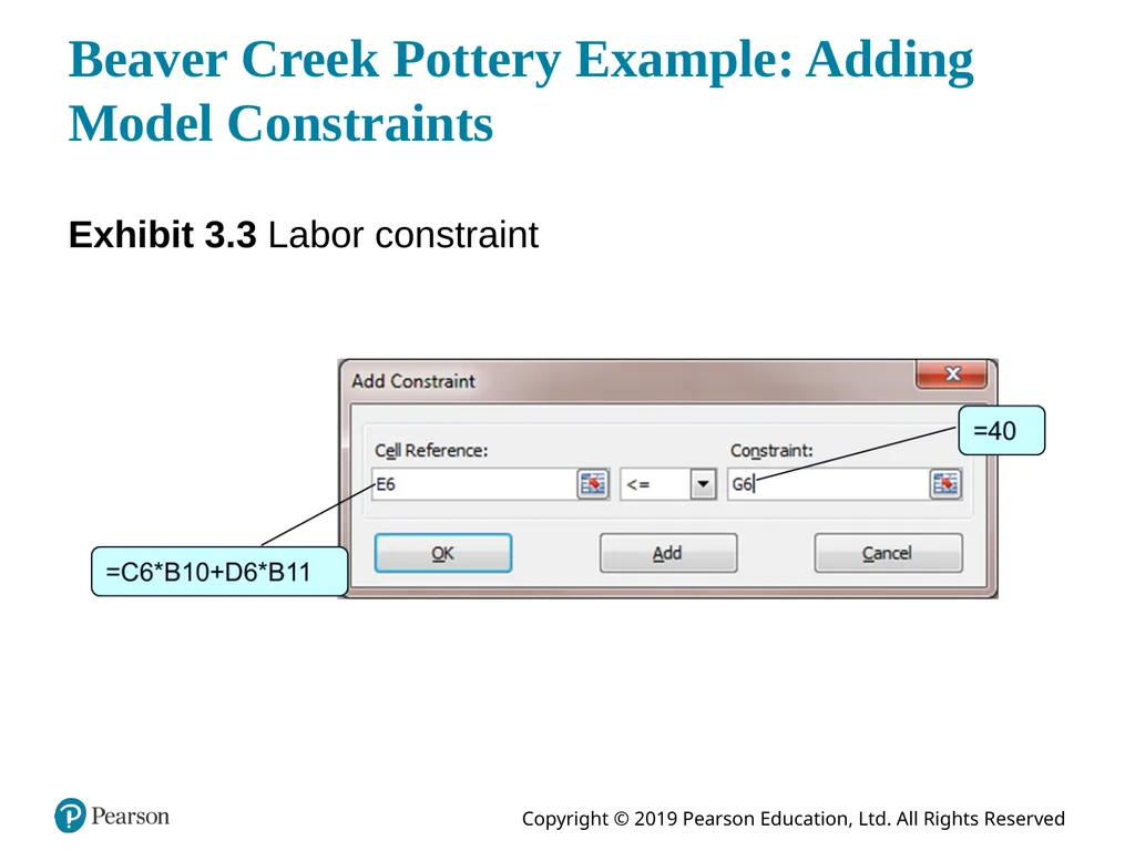
Beaver Creek Pottery Example: Adding Model Constraints Exhibit 3.3 Labor constraint

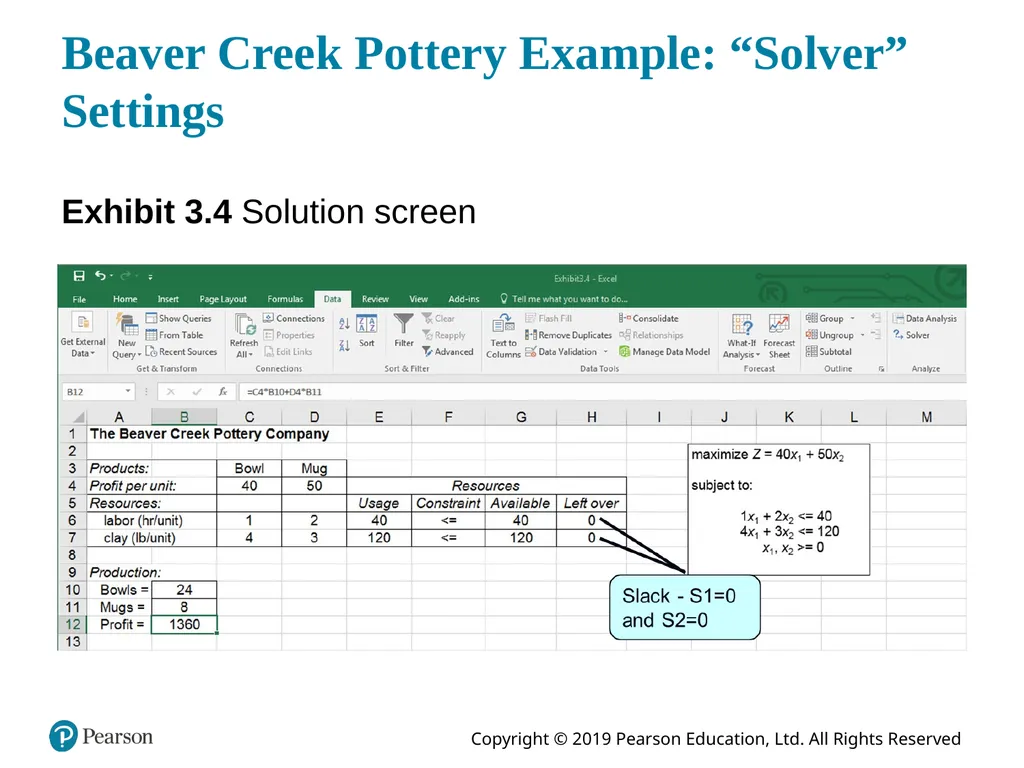
Beaver Creek Pottery Example: “Solver” Settings Exhibit 3.4 Solution screen

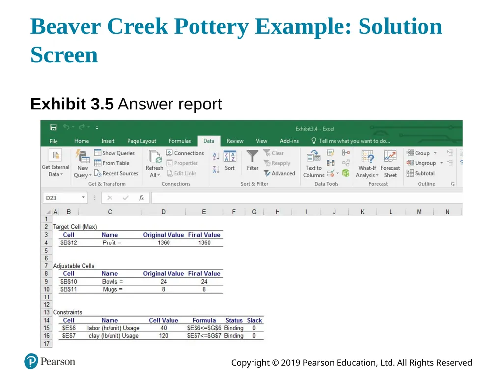
Beaver Creek Pottery Example: Solution Screen Exhibit 3.5 Answer report

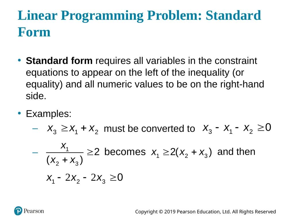
Linear Programming Problem: Standard Form Standard form requires all variables in the constraint equations to appear on the left of the inequality (or equality) and all numeric values to be on the right-hand side.
Examples: must be converted to and then

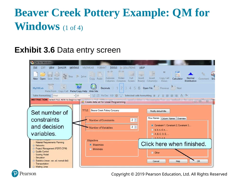
Beaver Creek Pottery Example: Q M for Windows (1 of 4) Exhibit 3.6 Data entry screen

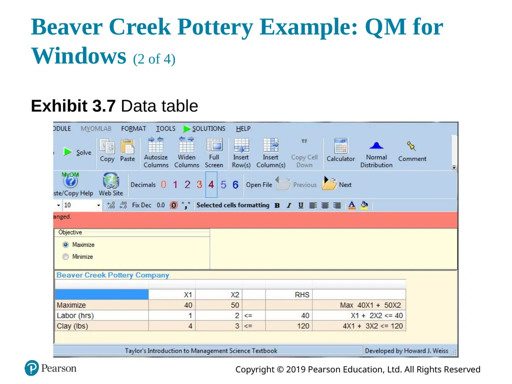
Beaver Creek Pottery Example: Q M for Windows (2 of 4) Exhibit 3.7 Data table

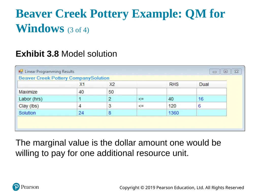
Beaver Creek Pottery Example: Q M for Windows (3 of 4) Exhibit 3.8 Model solution The marginal value is the dollar amount one would be willing to pay for one additional resource unit.

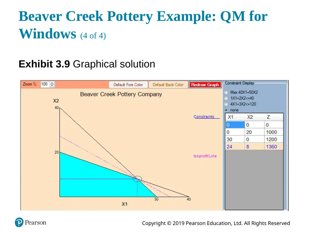
Beaver Creek Pottery Example: Q M for Windows (4 of 4) Exhibit 3.9 Graphical solution

Learning Objective 3.2 Sensitivity Analysis

Beaver Creek Pottery Example (1 of 2) Sensitivity analysis determines the effect on the optimal solution of changes in parameter values of the objective function and constraint equations.
Changes may be reactions to anticipated uncertainties in the parameters or to new or changed information concerning the model.

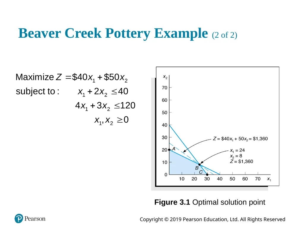
Beaver Creek Pottery Example (2 of 2) Figure 3.1 Optimal solution point

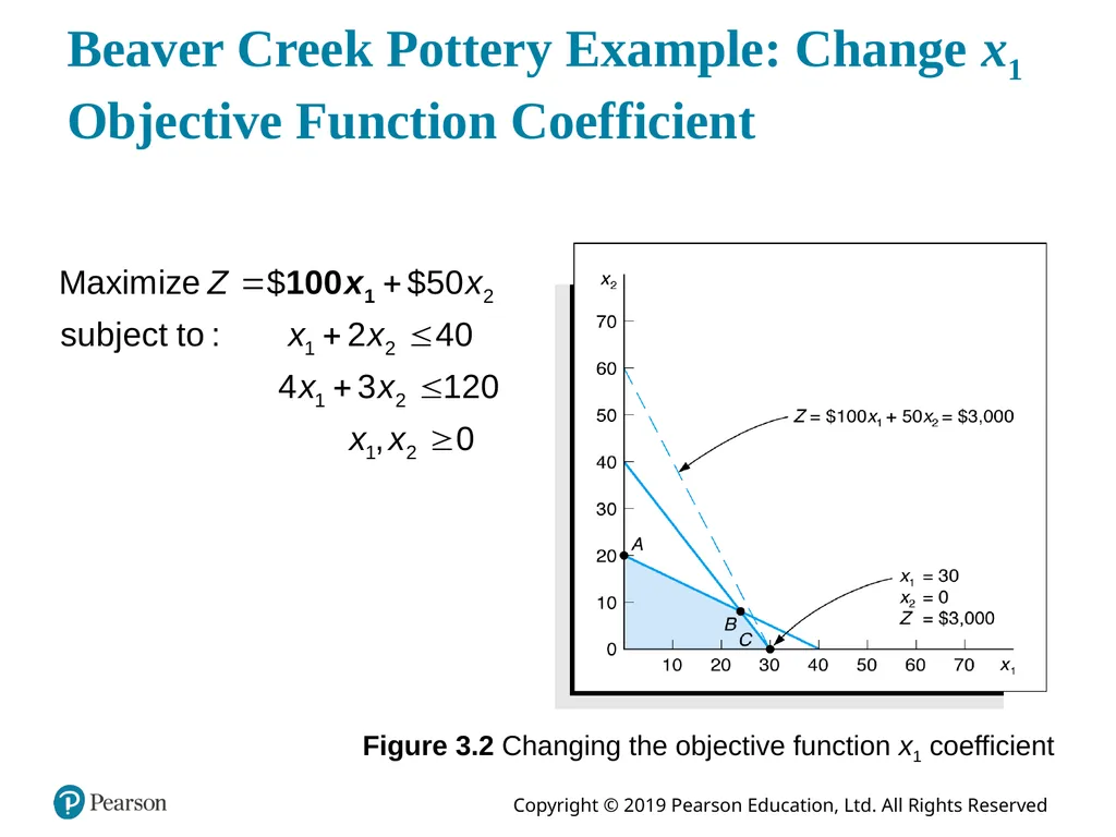
Beaver Creek Pottery Example: Change x1 Objective Function Coefficient Figure 3.2 Changing the objective function x1 coefficient

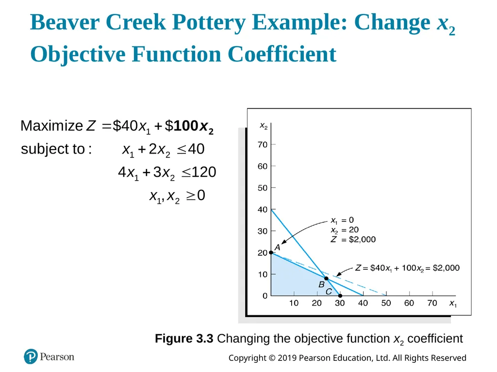
Beaver Creek Pottery Example: Change x2 Objective Function Coefficient Figure 3.3 Changing the objective function x2 coefficient

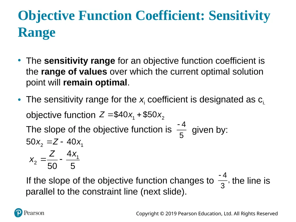
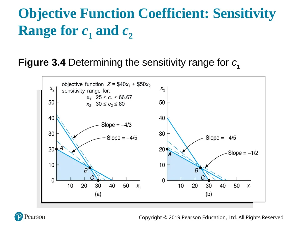
Objective Function Coefficient: Sensitivity Range The sensitivity range for an objective function coefficient is the range of values over which the current optimal solution point will remain optimal.
The sensitivity range for the xi coefficient is designated as ci. objective function The slope of the objective function is given by: If the slope of the objective function changes to the line is parallel to the constraint line (next slide).

Objective Function Coefficient: Sensitivity Range for c1 and c2 Figure 3.4 Determining the sensitivity range for c1

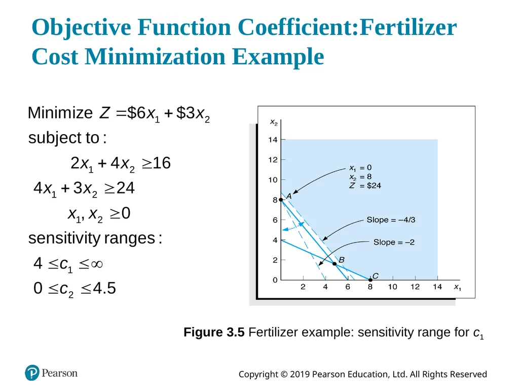
Objective Function Coefficient:Fertilizer Cost Minimization Example Figure 3.5 Fertilizer example: sensitivity range for c1

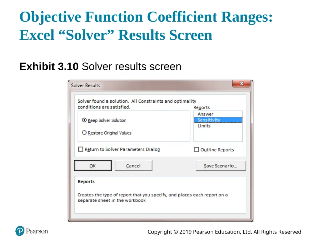
Objective Function Coefficient Ranges: Excel “Solver” Results Screen Exhibit 3.10 Solver results screen

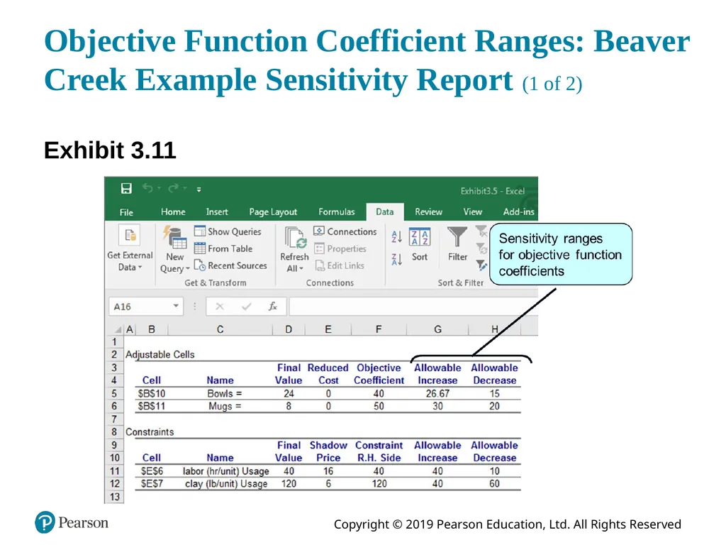
Objective Function Coefficient Ranges: Beaver Creek Example Sensitivity Report (1 of 2) Exhibit 3.11

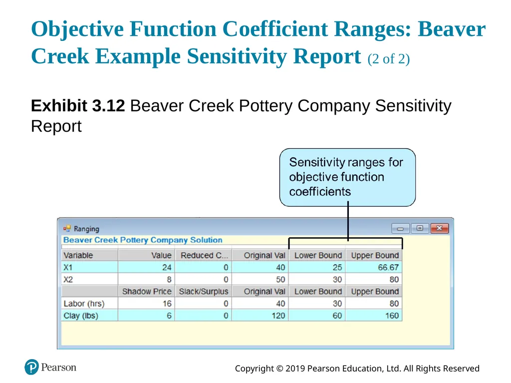
Objective Function Coefficient Ranges: Beaver Creek Example Sensitivity Report (2 of 2) Exhibit 3.12 Beaver Creek Pottery Company Sensitivity Report

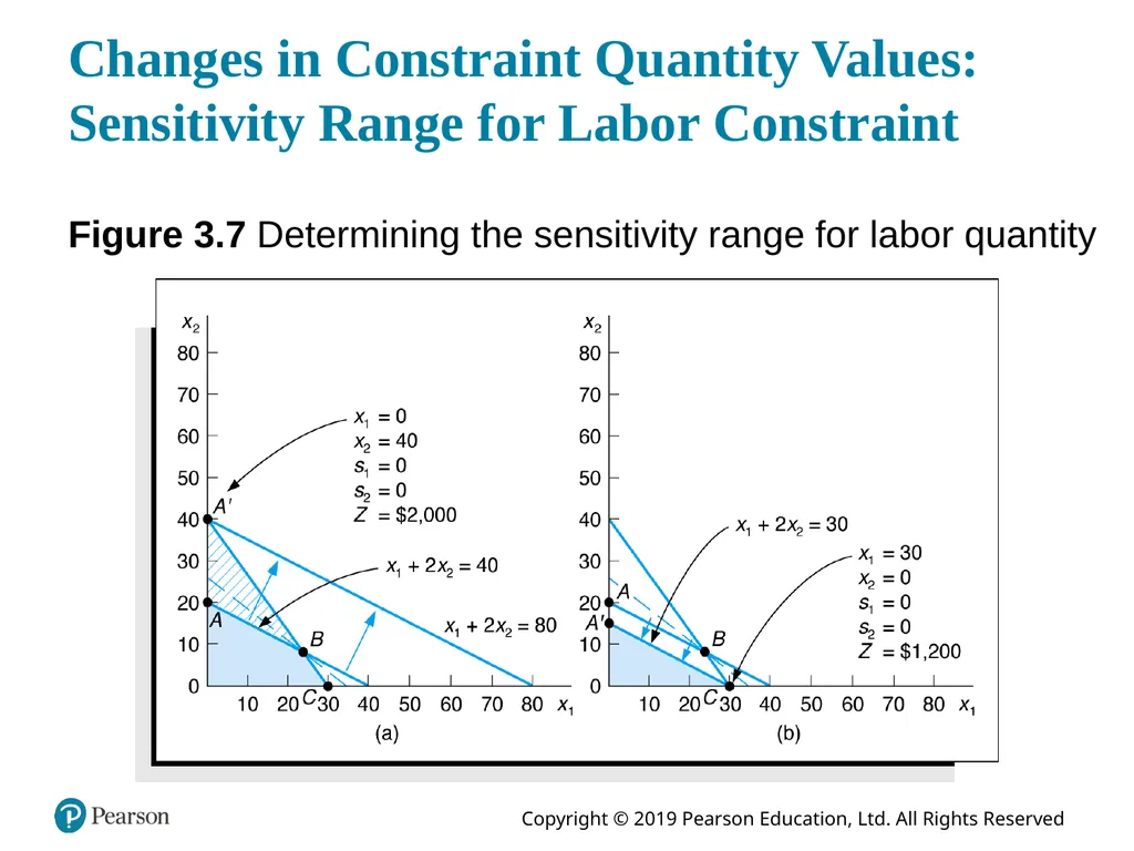
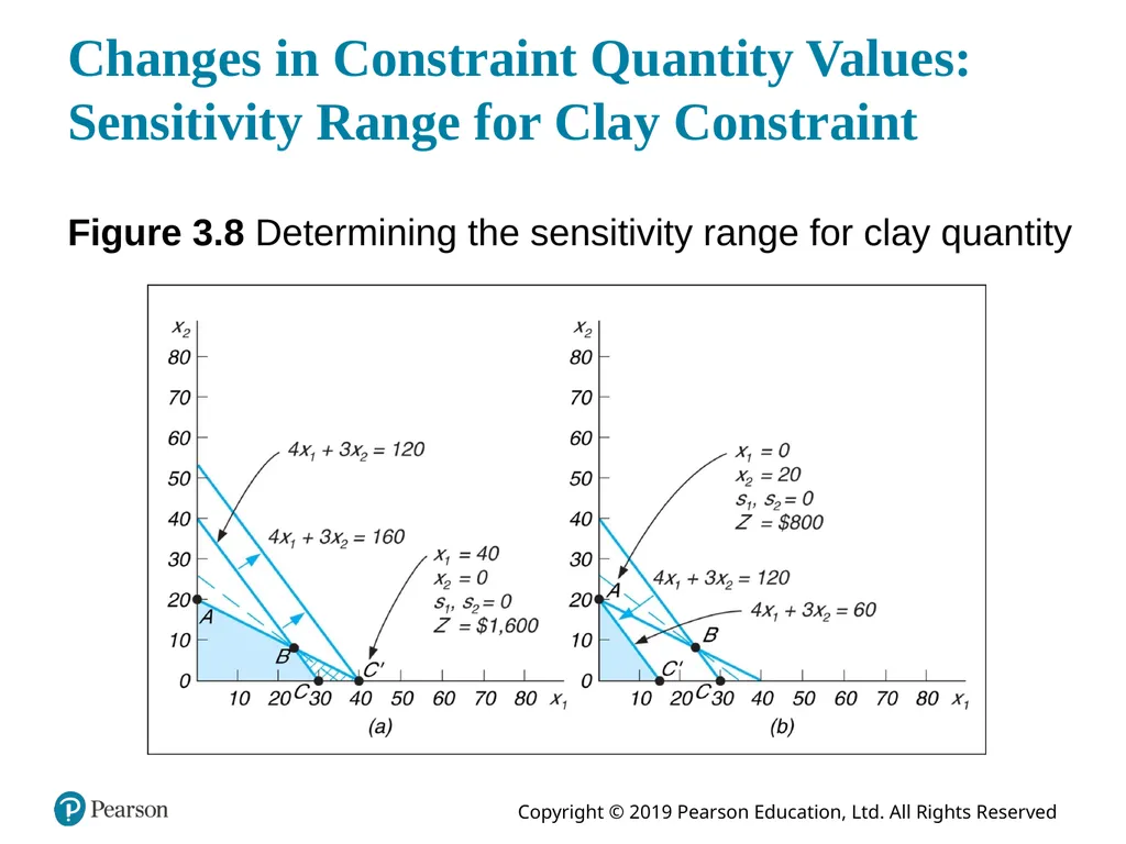
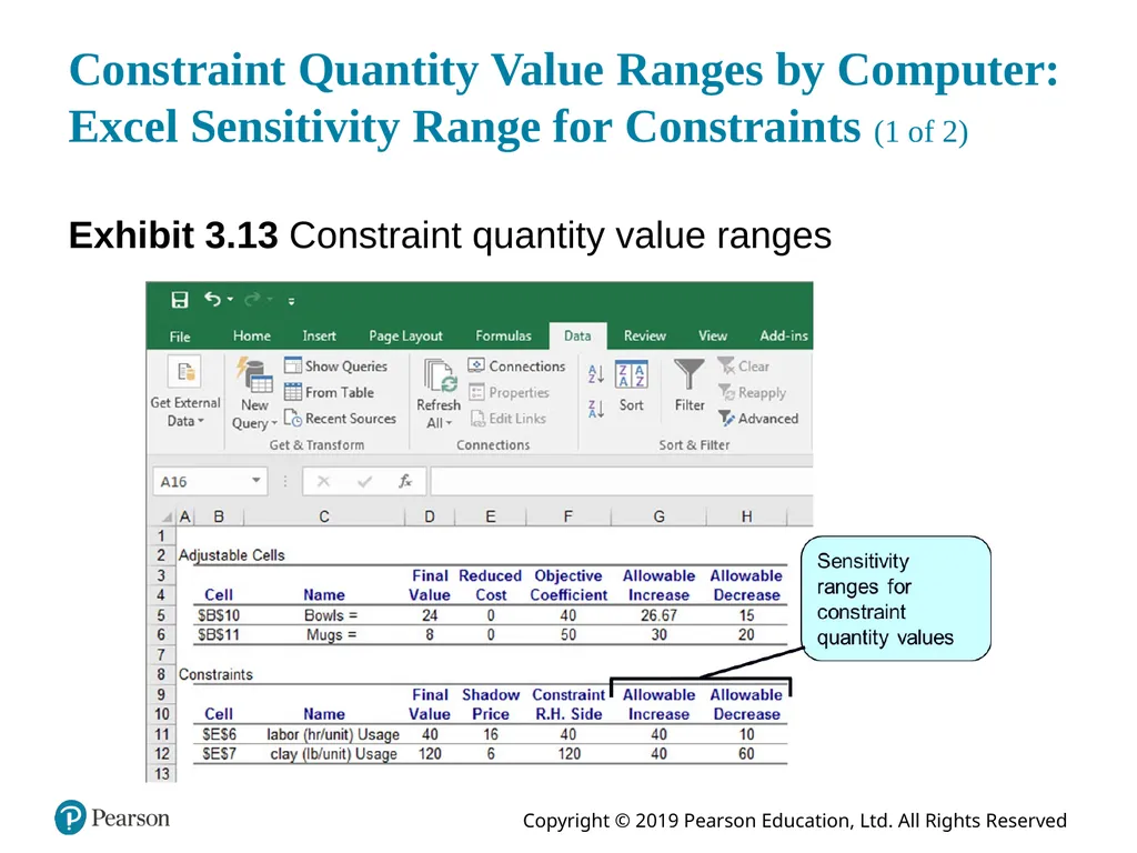
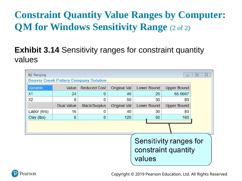
Changes in Constraint Quantity Values: Sensitivity Range The sensitivity range for a right-hand-side value is the range of values over which the quantity’s value can change without changing the solution variable mix, including the slack variables.
Recall the Beaver Creek Pottery example. Consider a change in which the manager can increase labor hours from 40 to 60.

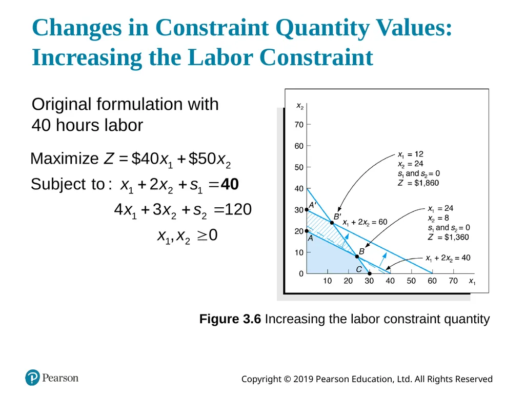
Changes in Constraint Quantity Values: Increasing the Labor Constraint Original formulation with 40 hours labor Figure 3.6 Increasing the labor constraint quantity

Changes in Constraint Quantity Values: Sensitivity Range for Labor Constraint Figure 3.7 Determining the sensitivity range for labor quantity

Changes in Constraint Quantity Values: Sensitivity Range for Clay Constraint Figure 3.8 Determining the sensitivity range for clay quantity

Constraint Quantity Value Ranges by Computer: Excel Sensitivity Range for Constraints (1 of 2) Exhibit 3.13 Constraint quantity value ranges

Constraint Quantity Value Ranges by Computer: Q M for Windows Sensitivity Range (2 of 2) Exhibit 3.14 Sensitivity ranges for constraint quantity values

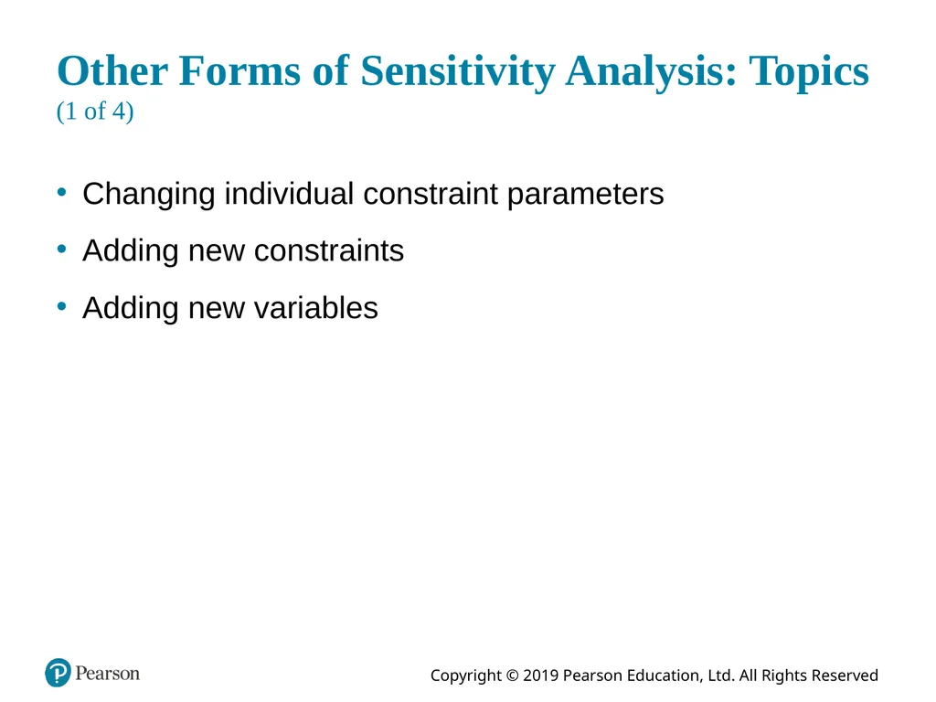
Other Forms of Sensitivity Analysis: Topics (1 of 4) Changing individual constraint parameters
Adding new constraints
Adding new variables

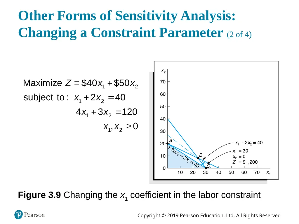
Other Forms of Sensitivity Analysis: Changing a Constraint Parameter (2 of 4) Figure 3.9 Changing the x1 coefficient in the labor constraint

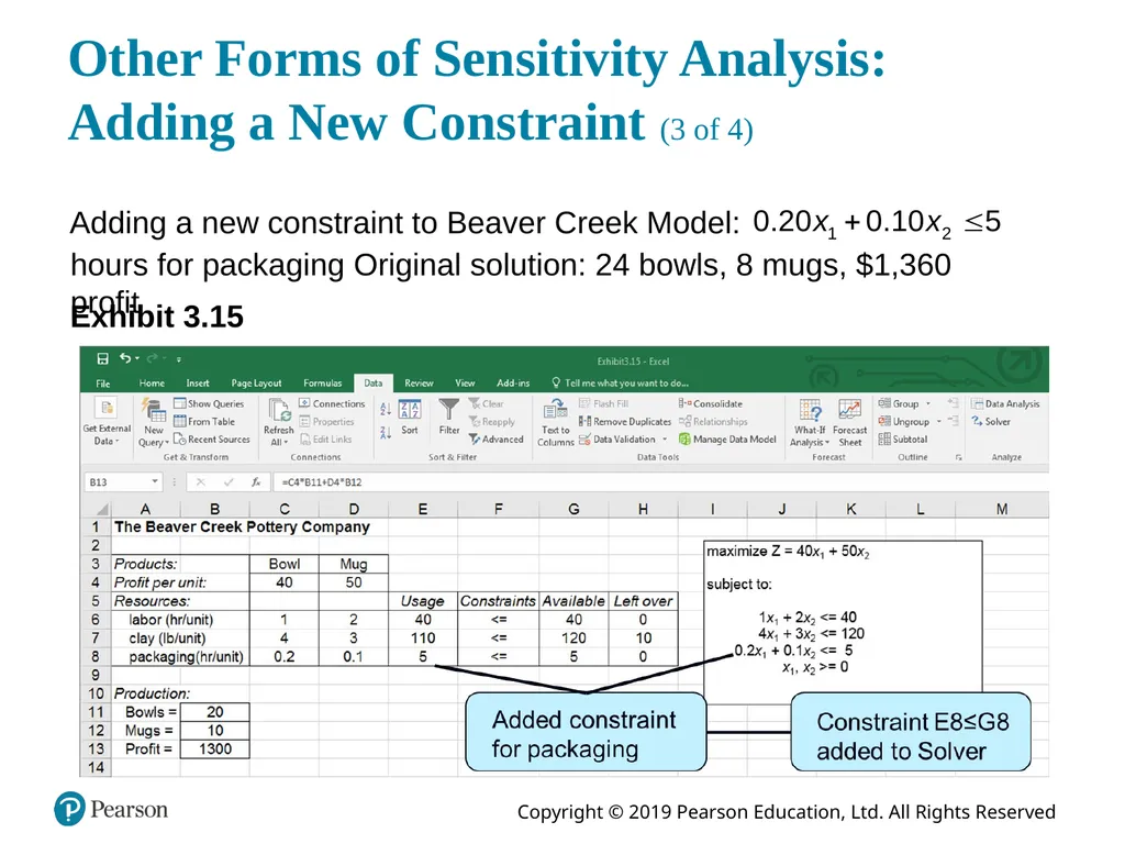
Other Forms of Sensitivity Analysis: Adding a New Constraint (3 of 4) Adding a new constraint to Beaver Creek Model: hours for packaging Original solution: 24 bowls, 8 mugs, $1,360 profit Exhibit 3.15

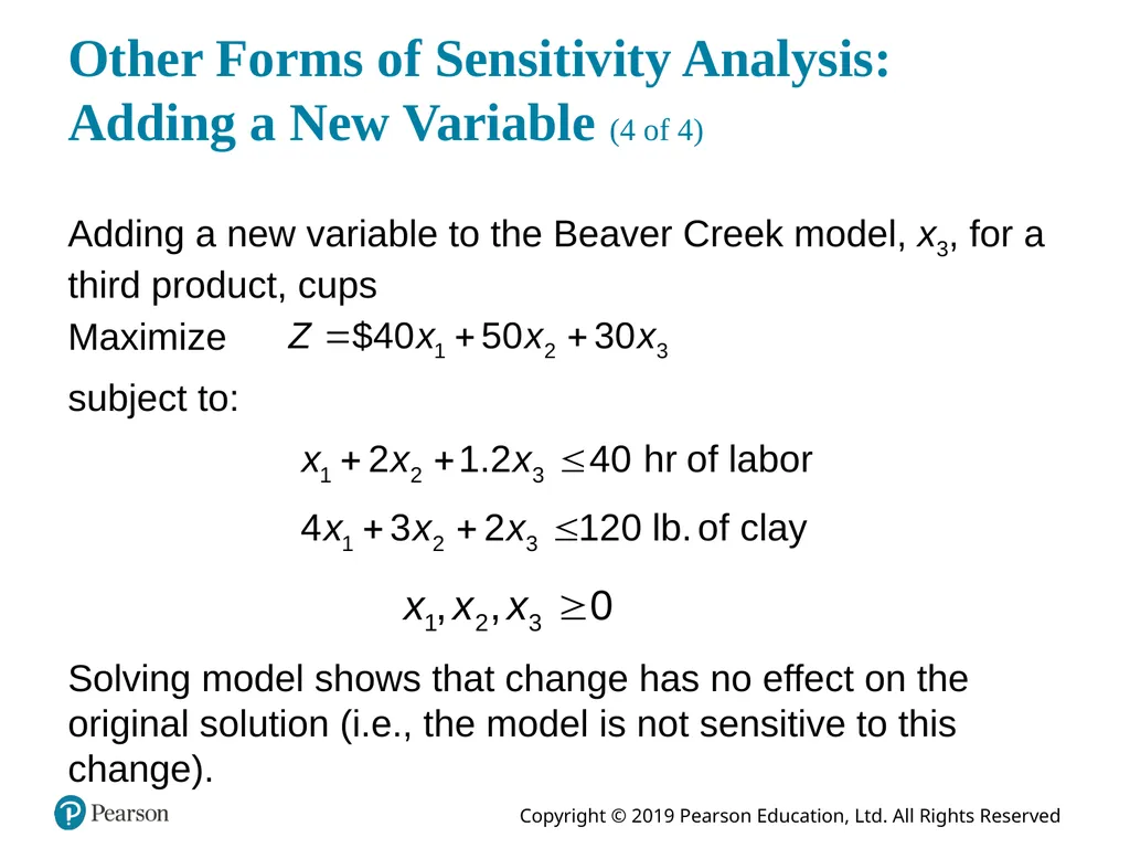
Other Forms of Sensitivity Analysis: Adding a New Variable (4 of 4) Adding a new variable to the Beaver Creek model, x3, for a third product, cups Maximize subject to: Solving model shows that change has no effect on the original solution (i.e., the model is not sensitive to this change).

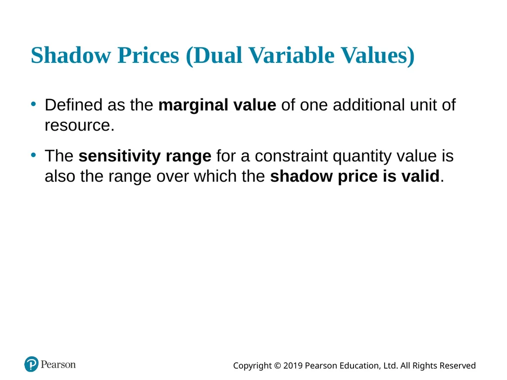
Shadow Prices (Dual Variable Values) Defined as the marginal value of one additional unit of resource.
The sensitivity range for a constraint quantity value is also the range over which the shadow price is valid.

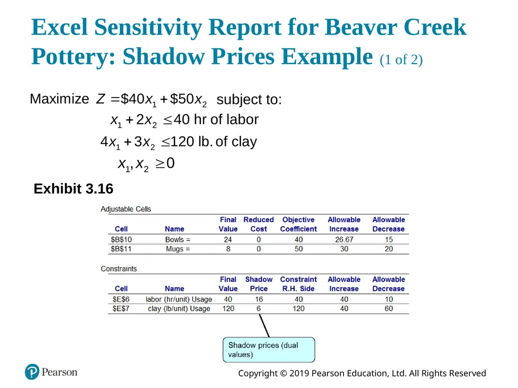
Excel Sensitivity Report for Beaver Creek Pottery: Shadow Prices Example (1 of 2) subject to: Exhibit 3.16

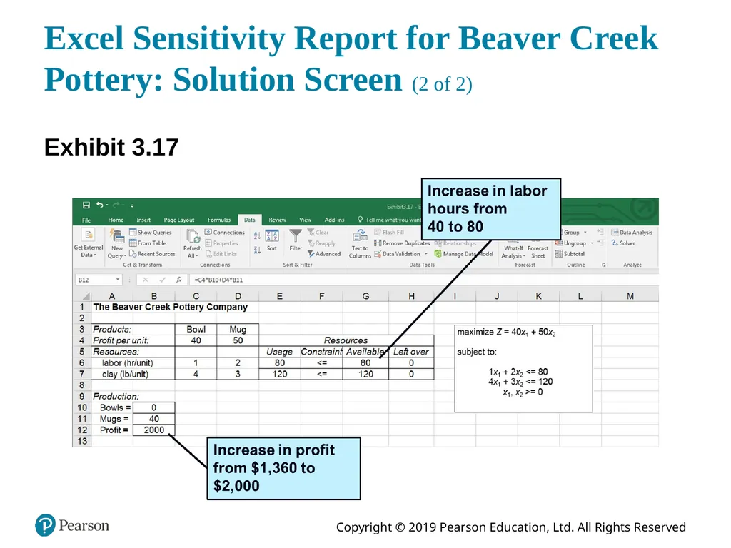
Excel Sensitivity Report for Beaver Creek Pottery: Solution Screen (2 of 2) Exhibit 3.17

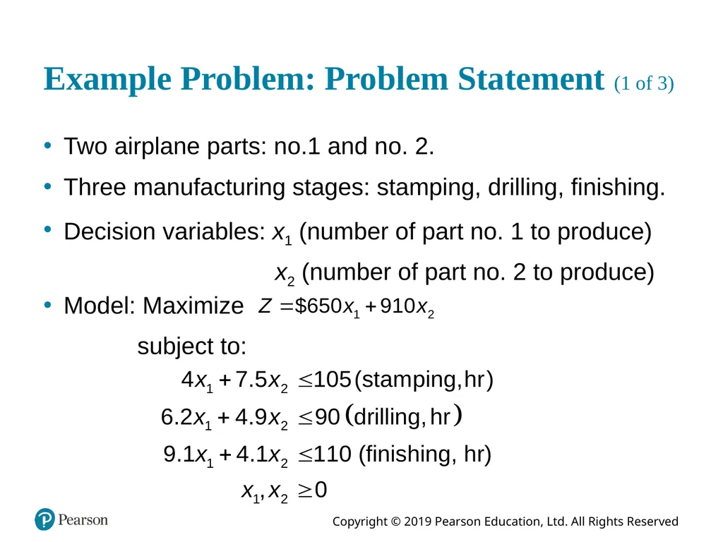
Example Problem: Problem Statement (1 of 3) Two airplane parts: n o.1 and n o. 2.
Three manufacturing stages: stamping, drilling, finishing.
Decision variables: x1 (number of part no. 1 to produce) x2 (number of part no. 2 to produce) Model: Maximize subject to:

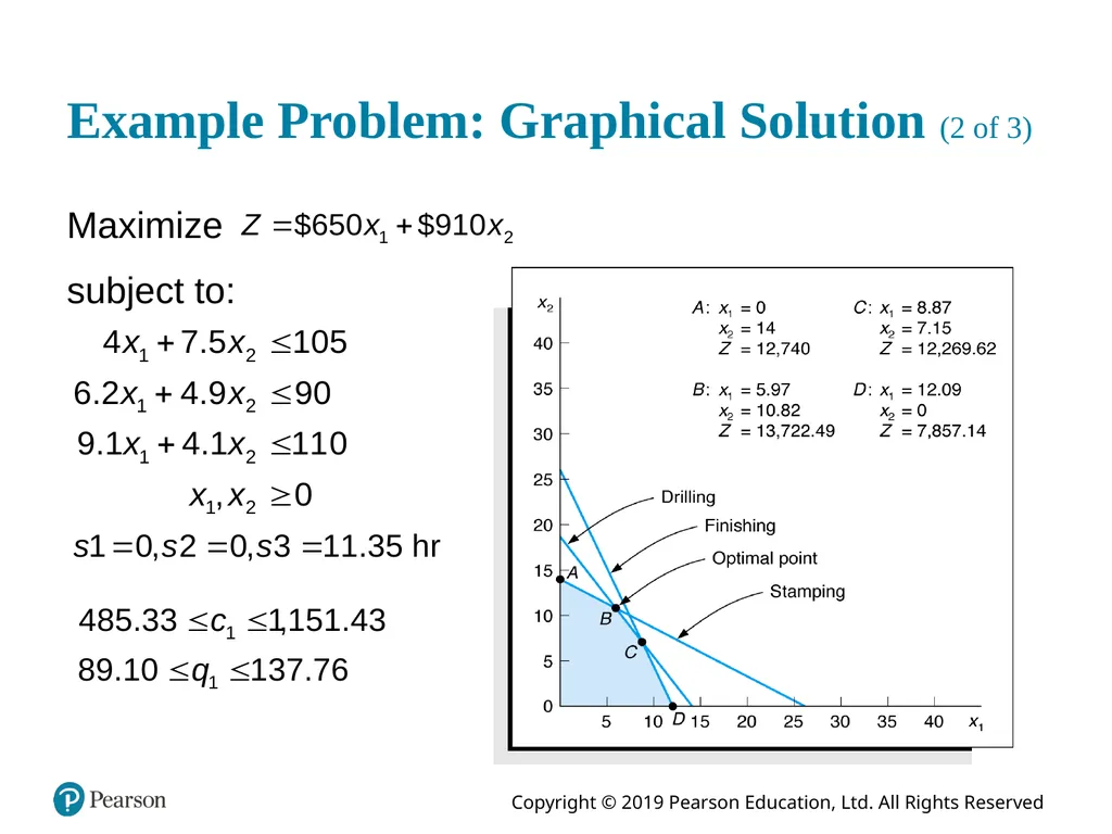
Example Problem: Graphical Solution (2 of 3) Maximize subject to:

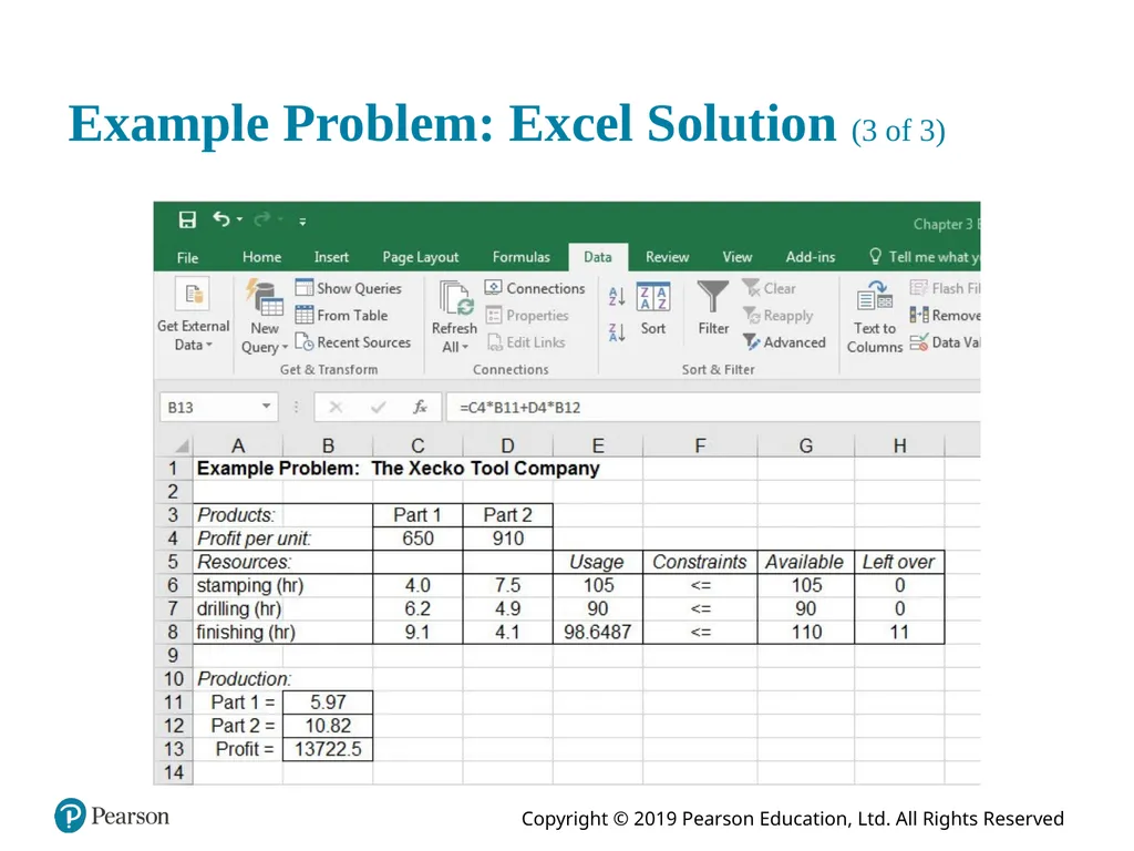
Example Problem: Excel Solution (3 of 3)

Introduction to Management Science Thirteenth

Related Topics

Share

Embed code

Download this presentation From Below

Presentation Transcript