Lecture 3 Sparse Direct Method: Combinatorics

yoshiko-marsland

Published 2026-08-14 · 35 slides · 0 views

↓ Download

Lecture 3 Sparse Direct Method: Combinatorics

Lecture 3 Sparse Direct Method: Combinatorics - slide 1 of 35

Lecture 3 Sparse Direct Method: Combinatorics - slide 2 of 35

Lecture 3 Sparse Direct Method: Combinatorics - slide 3 of 35

Lecture 3 Sparse Direct Method: Combinatorics - slide 4 of 35

Lecture 3 Sparse Direct Method: Combinatorics - slide 5 of 35

Lecture 3 Sparse Direct Method: Combinatorics - slide 6 of 35

Lecture 3 Sparse Direct Method: Combinatorics - slide 7 of 35

Lecture 3 Sparse Direct Method: Combinatorics - slide 8 of 35

Lecture 3 Sparse Direct Method: Combinatorics - slide 9 of 35

Lecture 3 Sparse Direct Method: Combinatorics - slide 10 of 35

Lecture 3 Sparse Direct Method: Combinatorics - slide 11 of 35

Lecture 3 Sparse Direct Method: Combinatorics - slide 12 of 35

Lecture 3 Sparse Direct Method: Combinatorics - slide 13 of 35

Lecture 3 Sparse Direct Method: Combinatorics - slide 14 of 35

Lecture 3 Sparse Direct Method: Combinatorics - slide 15 of 35

Lecture 3 Sparse Direct Method: Combinatorics - slide 16 of 35

Lecture 3 Sparse Direct Method: Combinatorics - slide 17 of 35

Lecture 3 Sparse Direct Method: Combinatorics - slide 18 of 35

Lecture 3 Sparse Direct Method: Combinatorics - slide 19 of 35

Lecture 3 Sparse Direct Method: Combinatorics - slide 20 of 35

Lecture 3 Sparse Direct Method: Combinatorics - slide 21 of 35

Lecture 3 Sparse Direct Method: Combinatorics - slide 22 of 35

Lecture 3 Sparse Direct Method: Combinatorics - slide 23 of 35

Lecture 3 Sparse Direct Method: Combinatorics - slide 24 of 35

Lecture 3 Sparse Direct Method: Combinatorics - slide 25 of 35

Lecture 3 Sparse Direct Method: Combinatorics - slide 26 of 35

Lecture 3 Sparse Direct Method: Combinatorics - slide 27 of 35

Lecture 3 Sparse Direct Method: Combinatorics - slide 28 of 35

Lecture 3 Sparse Direct Method: Combinatorics - slide 29 of 35

Lecture 3 Sparse Direct Method: Combinatorics - slide 30 of 35

Lecture 3 Sparse Direct Method: Combinatorics - slide 31 of 35

Lecture 3 Sparse Direct Method: Combinatorics - slide 32 of 35

Lecture 3 Sparse Direct Method: Combinatorics - slide 33 of 35

Lecture 3 Sparse Direct Method: Combinatorics - slide 34 of 35

Lecture 3 Sparse Direct Method: Combinatorics - slide 35 of 35

Description

Lecture 3 Sparse Direct Method: Combinatorics Xiaoye Sherry Li Lawrence Berkeley National Laboratory, USA xslilbl.gov crd-legacy.lbl.govxiaoyeG2S3 4th Gene Golub SIAM Summer School, 722 87, 2013, Shanghai Lecture outline Linear

Download this presentation From Below

"Lecture 3 Sparse Direct Method: Combinatorics" is the property of its rightful owner. Permission is granted to download and print the materials on this website for personal, non-commercial use only, and to display it on your personal computer provided you do not modify the materials and that you retain all copyright notices contained in the materials. By downloading content from our website, you accept the terms of this agreement.

Presentation Transcript

Lecture 3 Sparse Direct Method: Combinatorics Xiaoye Sherry Li
Lawrence Berkeley National Laboratory, USA
xsli@lbl.gov

crd-legacy.lbl.gov/~xiaoye/G2S3/ 4th Gene Golub SIAM Summer School, 7/22 – 8/7, 2013, Shanghai

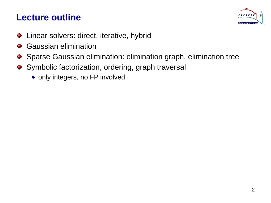
Lecture outline Linear solvers: direct, iterative, hybrid
Gaussian elimination
Sparse Gaussian elimination: elimination graph, elimination tree
Symbolic factorization, ordering, graph traversal
only integers, no FP involved 2

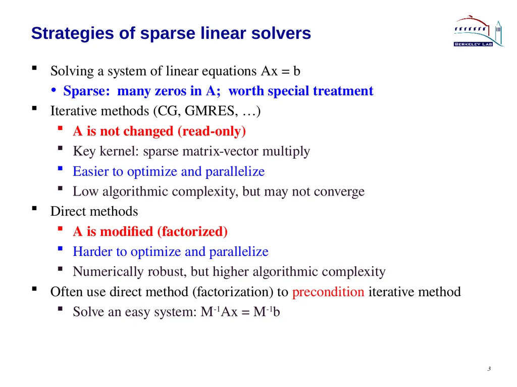
Solving a system of linear equations Ax = b
Sparse: many zeros in A; worth special treatment
Iterative methods (CG, GMRES, …)
A is not changed (read-only)
Key kernel: sparse matrix-vector multiply
Easier to optimize and parallelize
Low algorithmic complexity, but may not converge
Direct methods
A is modified (factorized)
Harder to optimize and parallelize
Numerically robust, but higher algorithmic complexity
Often use direct method (factorization) to precondition iterative method
Solve an easy system: M-1Ax = M-1b Strategies of sparse linear solvers 3

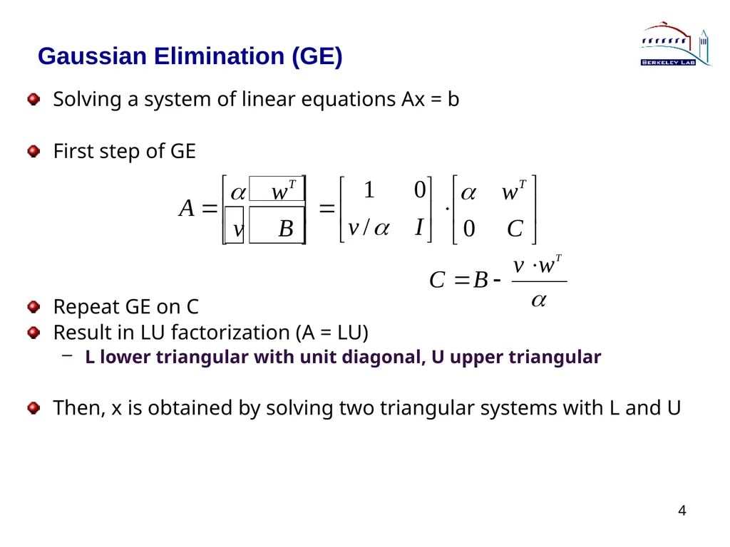
Gaussian Elimination (GE) Solving a system of linear equations Ax = b

First step of GE

Repeat GE on C
Result in LU factorization (A = LU)
L lower triangular with unit diagonal, U upper triangular

Then, x is obtained by solving two triangular systems with L and U 4

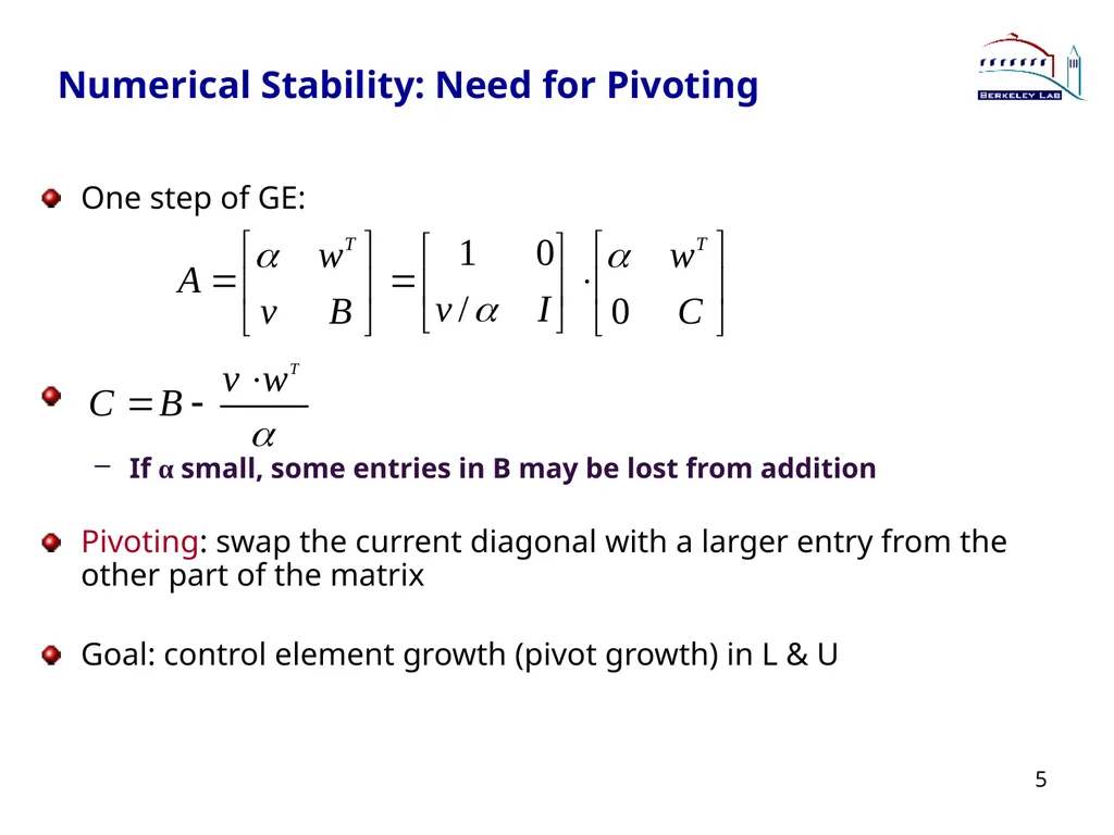
Numerical Stability: Need for Pivoting One step of GE:

If α small, some entries in B may be lost from addition

Pivoting: swap the current diagonal with a larger entry from the other part of the matrix

Goal: control element growth (pivot growth) in L & U 5

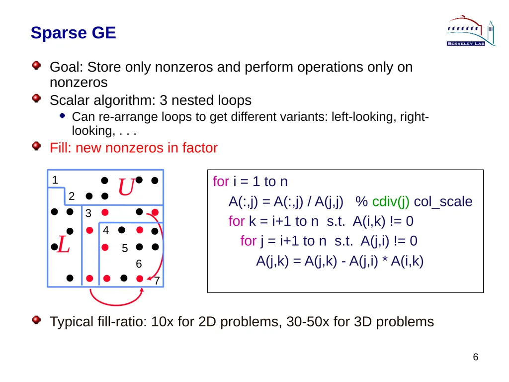
Sparse GE Goal: Store only nonzeros and perform operations only on nonzeros
Scalar algorithm: 3 nested loops
Can re-arrange loops to get different variants: left-looking, right-looking, . . .
Fill: new nonzeros in factor

Typical fill-ratio: 10x for 2D problems, 30-50x for 3D problems 6 for i = 1 to n
A(:,j) = A(:,j) / A(j,j) % cdiv(j) col_scale
for k = i+1 to n s.t. A(i,k) != 0
for j = i+1 to n s.t. A(j,i) != 0
A(j,k) = A(j,k) - A(j,i) * A(i,k)

Useful tool to discover fill: Reachable Set Given certain elimination order (x1, x2, . . ., xn), how do you determine the fill-ins using original graph of A ?
An implicit elimination model
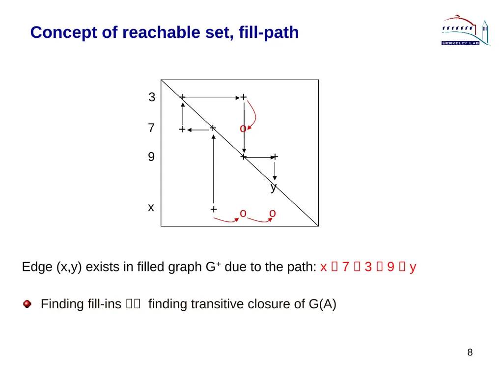
Definition: Let S be a subset of the node set. The reachable set of y through S is:
Reach(y, S) = { x | there exists a directed path (y,v1,…vk, x), vi in S}

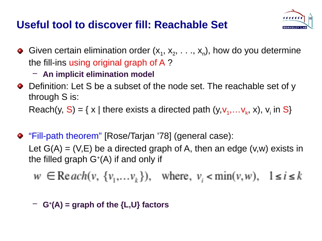
“Fill-path theorem” [Rose/Tarjan ’78] (general case):
Let G(A) = (V,E) be a directed graph of A, then an edge (v,w) exists in the filled graph G+(A) if and only if

G+(A) = graph of the {L,U} factors

8 Concept of reachable set, fill-path Edge (x,y) exists in filled graph G+ due to the path: x  7  3  9  y

Finding fill-ins  finding transitive closure of G(A)

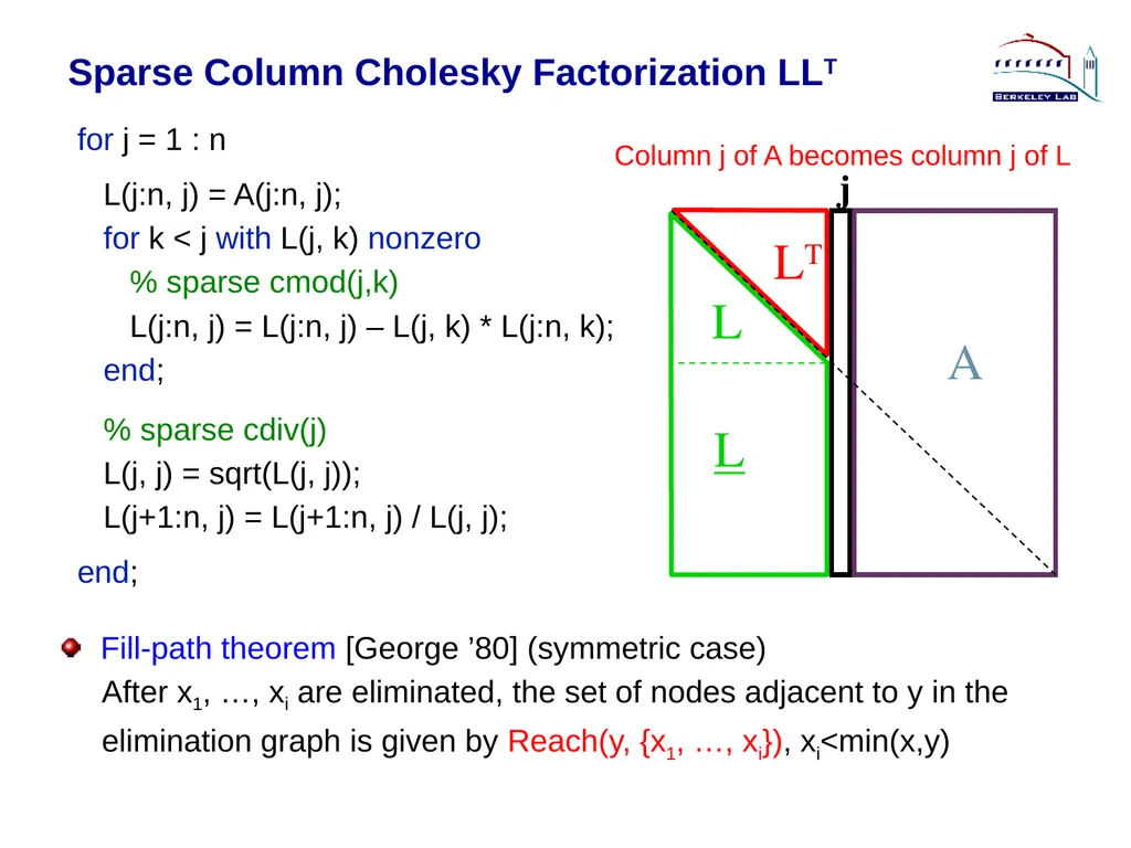
Sparse Column Cholesky Factorization LLT for j = 1 : n

L(j:n, j) = A(j:n, j);
for k < j with L(j, k) nonzero
% sparse cmod(j,k)
L(j:n, j) = L(j:n, j) – L(j, k) * L(j:n, k);
end;

% sparse cdiv(j)
L(j, j) = sqrt(L(j, j));
L(j+1:n, j) = L(j+1:n, j) / L(j, j);

end; Column j of A becomes column j of L Fill-path theorem [George ’80] (symmetric case)
After x1, …, xi are eliminated, the set of nodes adjacent to y in the
elimination graph is given by Reach(y, {x1, …, xi}), xi<min(x,y)

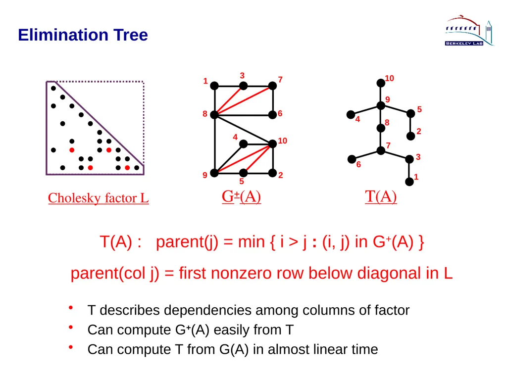
Elimination Tree Cholesky factor L G+(A) T(A) T(A) : parent(j) = min { i > j : (i, j) in G+(A) }

parent(col j) = first nonzero row below diagonal in L

T describes dependencies among columns of factor
Can compute G+(A) easily from T
Can compute T from G(A) in almost linear time

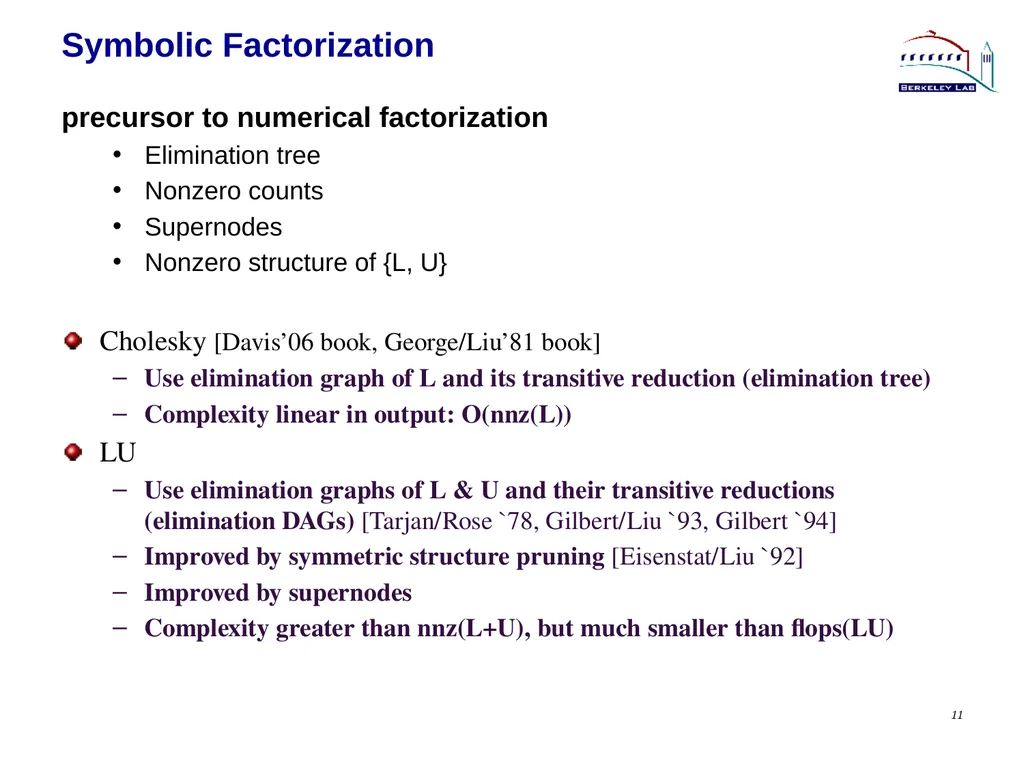
11 Symbolic Factorization precursor to numerical factorization
Elimination tree
Nonzero counts
Supernodes
Nonzero structure of {L, U}

Cholesky [Davis’06 book, George/Liu’81 book]
Use elimination graph of L and its transitive reduction (elimination tree)
Complexity linear in output: O(nnz(L))
LU
Use elimination graphs of L & U and their transitive reductions (elimination DAGs) [Tarjan/Rose `78, Gilbert/Liu `93, Gilbert `94]
Improved by symmetric structure pruning [Eisenstat/Liu `92]
Improved by supernodes
Complexity greater than nnz(L+U), but much smaller than flops(LU)

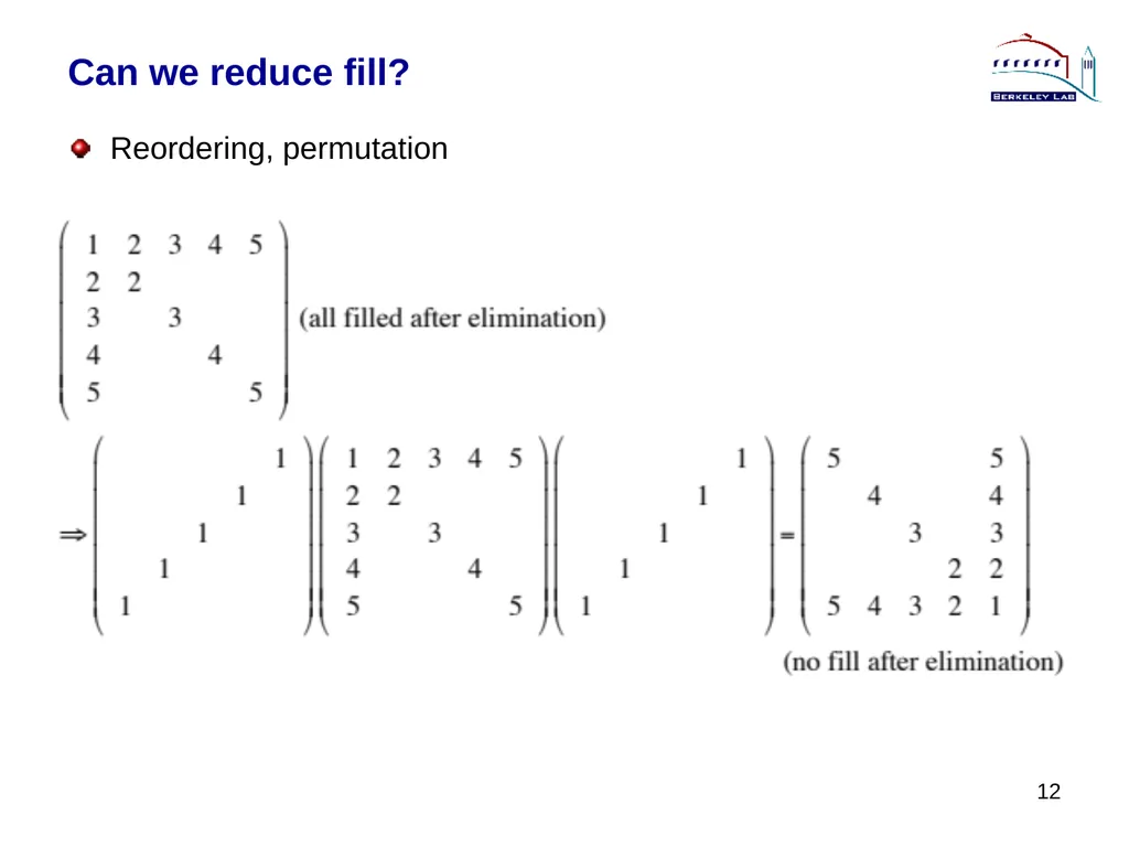
Can we reduce fill? Reordering, permutation 12

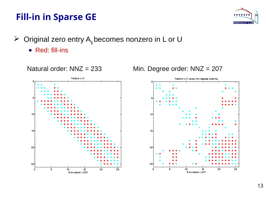
Fill-in in Sparse GE Original zero entry Aij becomes nonzero in L or U
Red: fill-ins

Natural order: NNZ = 233 Min. Degree order: NNZ = 207 13

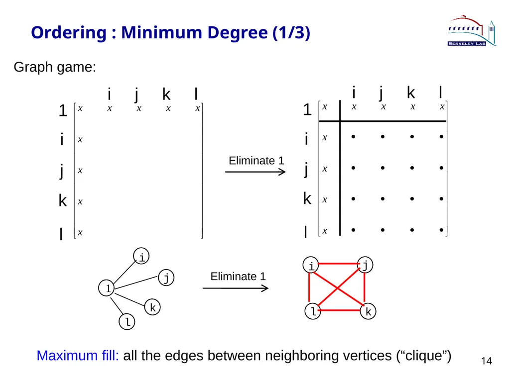
Ordering : Minimum Degree (1/3) Graph game: i j k l 1 i j k l 14 Maximum fill: all the edges between neighboring vertices (“clique”)

Minimum Degree Ordering (2/3) Greedy approach: do the best locally
Best for modest size problems
Hard to parallelize

At each step
Eliminate the vertex with the smallest degree
Update degrees of the neighbors

Straightforward implementation is slow and requires too much memory
Newly added edges are more than eliminated vertices 15

Minimum Degree Ordering (3/3) Use quotient graph (QG) as a compact representation [George/Liu ’78]
Collection of cliques resulting from the eliminated vertices affects the degree of an uneliminated vertex
Represent each connected component in the eliminated subgraph by a single “supervertex”
Storage required to implement QG model is bounded by size of A
Large body of literature on implementation variants
Tinney/Walker `67, George/Liu `79, Liu `85, Amestoy/Davis/Duff `94, Ashcraft `95, Duff/Reid `95, et al., . .

Extended the QG model to nonsymmetric using bipartite graph [Amestoy/Li/Ng `07] 16

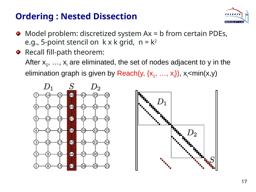
Ordering : Nested Dissection Model problem: discretized system Ax = b from certain PDEs, e.g., 5-point stencil on k x k grid, n = k2
Recall fill-path theorem:
After x1, …, xi are eliminated, the set of nodes adjacent to y in the
elimination graph is given by Reach(y, {x1, …, xi}), xi<min(x,y) 17

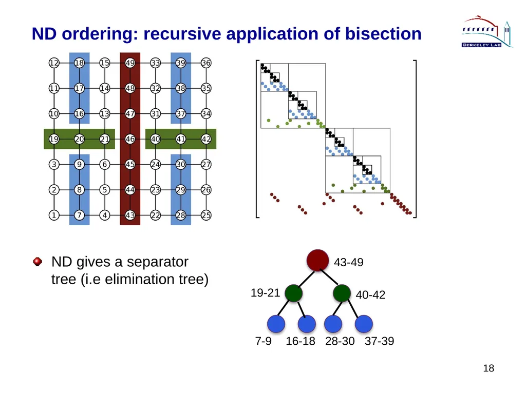
ND ordering: recursive application of bisection 18 ND gives a separator tree (i.e elimination tree)

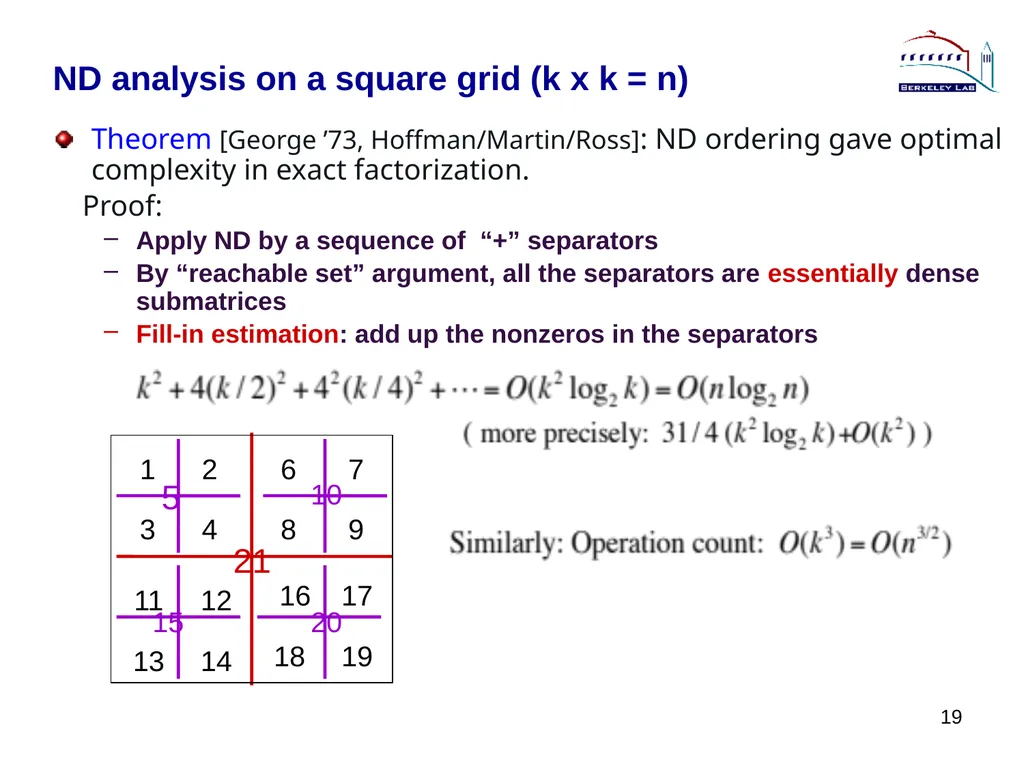
19 ND analysis on a square grid (k x k = n) Theorem [George ’73, Hoffman/Martin/Ross]: ND ordering gave optimal complexity in exact factorization.
Proof:
Apply ND by a sequence of “+” separators
By “reachable set” argument, all the separators are essentially dense submatrices
Fill-in estimation: add up the nonzeros in the separators

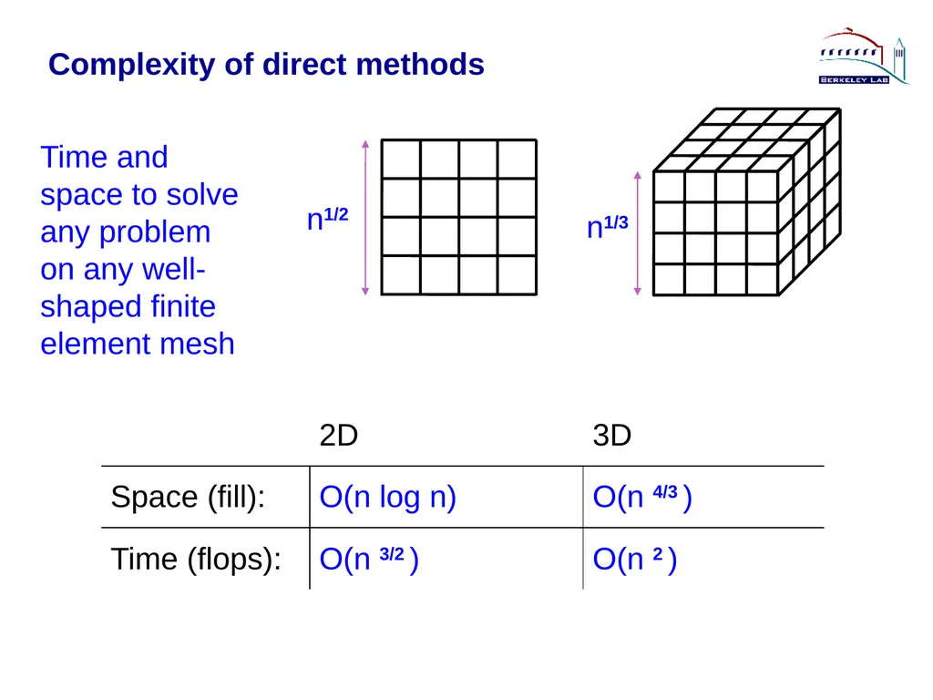
Complexity of direct methods Time and space to solve any problem on any well-shaped finite element mesh

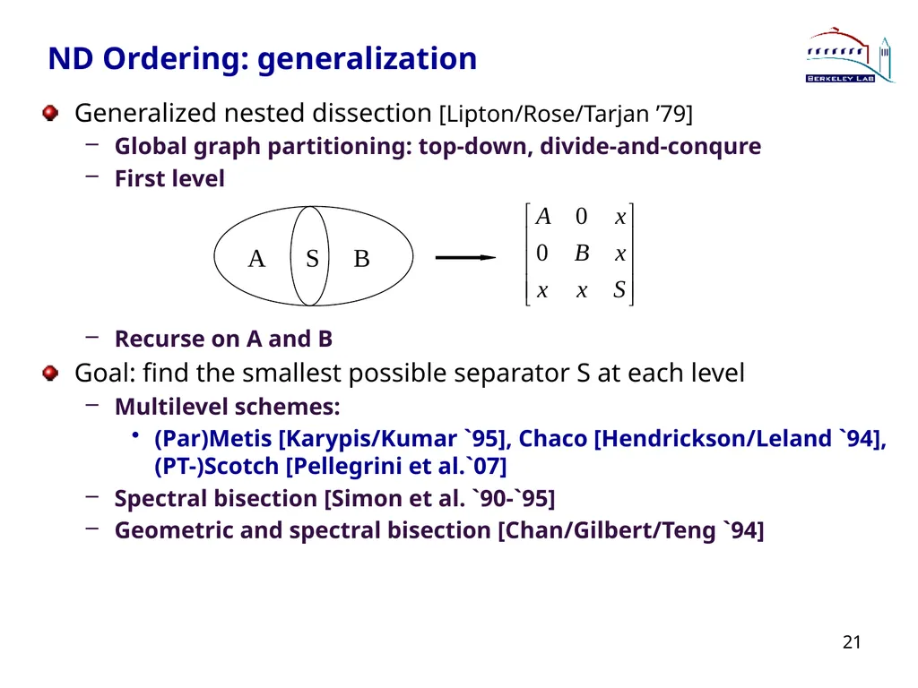
ND Ordering: generalization Generalized nested dissection [Lipton/Rose/Tarjan ’79]
Global graph partitioning: top-down, divide-and-conqure
First level

Recurse on A and B
Goal: find the smallest possible separator S at each level
Multilevel schemes:
(Par)Metis [Karypis/Kumar `95], Chaco [Hendrickson/Leland `94], (PT-)Scotch [Pellegrini et al.`07]
Spectral bisection [Simon et al. `90-`95]
Geometric and spectral bisection [Chan/Gilbert/Teng `94] 21

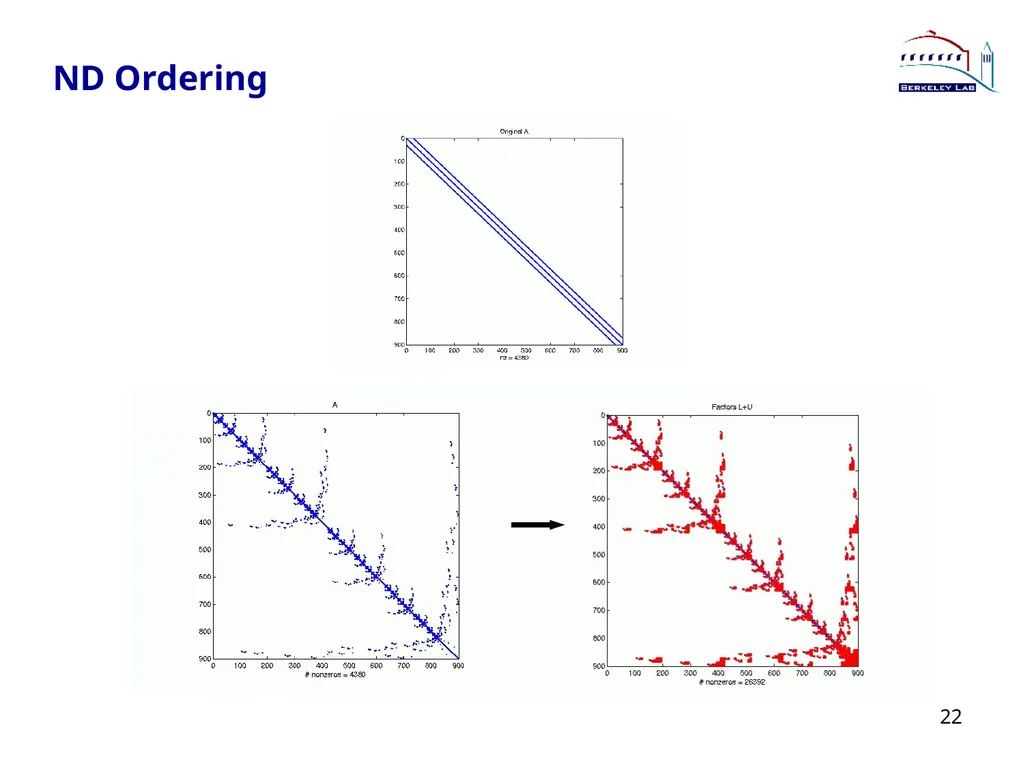
ND Ordering 22

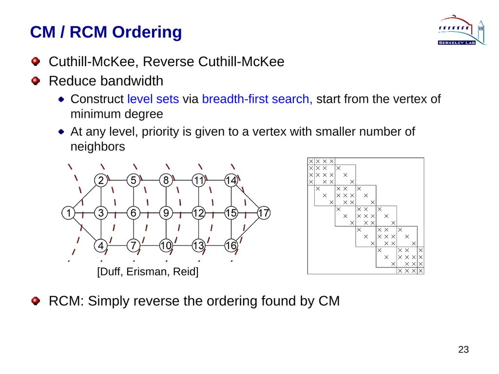
CM / RCM Ordering Cuthill-McKee, Reverse Cuthill-McKee
Reduce bandwidth
Construct level sets via breadth-first search, start from the vertex of minimum degree
At any level, priority is given to a vertex with smaller number of neighbors

RCM: Simply reverse the ordering found by CM 23 [Duff, Erisman, Reid]

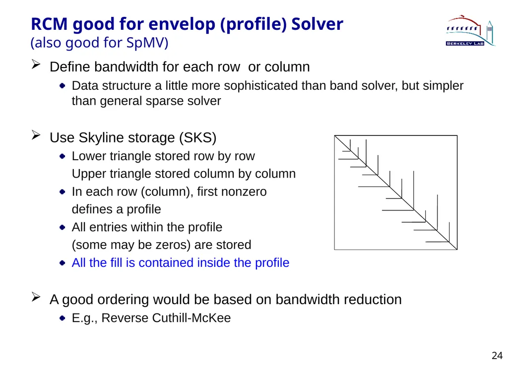
RCM good for envelop (profile) Solver(also good for SpMV) Define bandwidth for each row or column
Data structure a little more sophisticated than band solver, but simpler than general sparse solver

Use Skyline storage (SKS)
Lower triangle stored row by row
Upper triangle stored column by column
In each row (column), first nonzero
defines a profile
All entries within the profile
(some may be zeros) are stored
All the fill is contained inside the profile

A good ordering would be based on bandwidth reduction
E.g., Reverse Cuthill-McKee 24

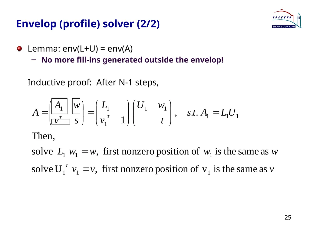
Envelop (profile) solver (2/2) Lemma: env(L+U) = env(A)
No more fill-ins generated outside the envelop!

Inductive proof: After N-1 steps, 25

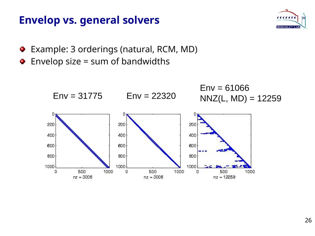
Envelop vs. general solvers Example: 3 orderings (natural, RCM, MD)
Envelop size = sum of bandwidths 26 Env = 31775 Env = 22320 Env = 61066
NNZ(L, MD) = 12259

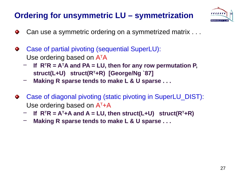
27 Ordering for unsymmetric LU – symmetrization Can use a symmetric ordering on a symmetrized matrix . . .

Case of partial pivoting (sequential SuperLU):
Use ordering based on ATA
If RTR = ATA and PA = LU, then for any row permutation P,
struct(L+U)  struct(RT+R) [George/Ng `87]
Making R sparse tends to make L & U sparse . . .

Case of diagonal pivoting (static pivoting in SuperLU_DIST):
Use ordering based on AT+A
If RTR = AT+A and A = LU, then struct(L+U)  struct(RT+R)
Making R sparse tends to make L & U sparse . . .

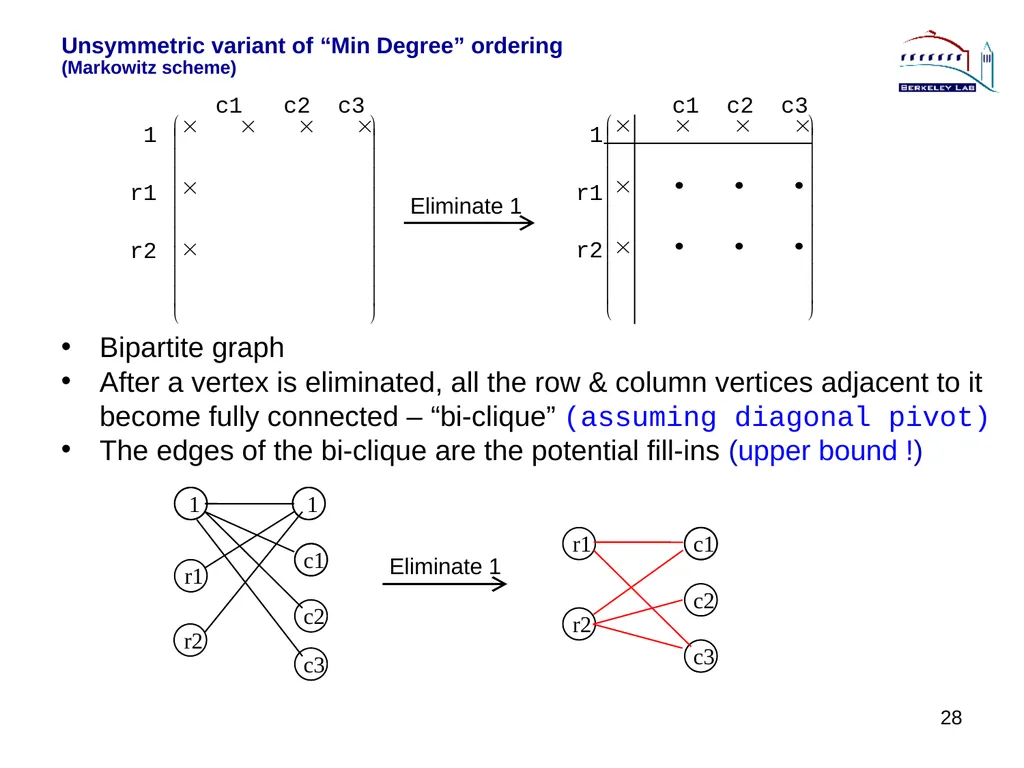
28 Unsymmetric variant of “Min Degree” ordering(Markowitz scheme)

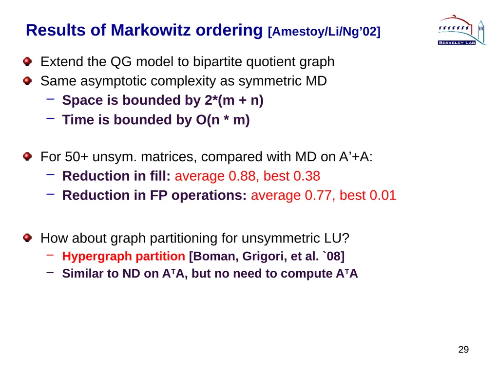
29 Results of Markowitz ordering [Amestoy/Li/Ng’02] Extend the QG model to bipartite quotient graph
Same asymptotic complexity as symmetric MD
Space is bounded by 2*(m + n)
Time is bounded by O(n * m)

For 50+ unsym. matrices, compared with MD on A’+A:
Reduction in fill: average 0.88, best 0.38
Reduction in FP operations: average 0.77, best 0.01

How about graph partitioning for unsymmetric LU?
Hypergraph partition [Boman, Grigori, et al. `08]
Similar to ND on ATA, but no need to compute ATA

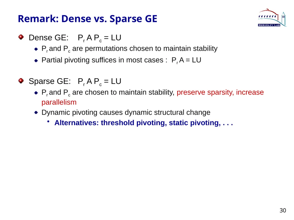
Remark: Dense vs. Sparse GE Dense GE: Pr A Pc = LU
Pr and Pc are permutations chosen to maintain stability
Partial pivoting suffices in most cases : Pr A = LU

Sparse GE: Pr A Pc = LU
Pr and Pc are chosen to maintain stability, preserve sparsity, increase parallelism
Dynamic pivoting causes dynamic structural change
Alternatives: threshold pivoting, static pivoting, . . . 30

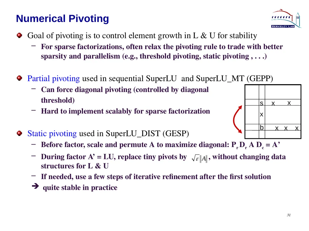
31 Numerical Pivoting Goal of pivoting is to control element growth in L & U for stability
For sparse factorizations, often relax the pivoting rule to trade with better sparsity and parallelism (e.g., threshold pivoting, static pivoting , . . .)

Partial pivoting used in sequential SuperLU and SuperLU_MT (GEPP)
Can force diagonal pivoting (controlled by diagonal
threshold)
Hard to implement scalably for sparse factorization

Static pivoting used in SuperLU_DIST (GESP)
Before factor, scale and permute A to maximize diagonal: Pr Dr A Dc = A’
During factor A’ = LU, replace tiny pivots by , without changing data structures for L & U
If needed, use a few steps of iterative refinement after the first solution
quite stable in practice

Use many heuristics Finding an optimal fill-reducing ordering is NP-complete  use heuristics:
Local approach: Minimum degree
Global approach: Nested dissection (optimal in special case), RCM
Hybrid: First permute the matrix globally to confine the fill-in, then reorder small parts using local heuristics
Local methods effective for smaller graph, global methods effective for larger graph

Numerical pivoting: trade-off stability with sparsity and parallelism
Partial pivoting too restrictive
Threshold pivoting
Static pivoting
… 32

Algorithmic phases in sparse GE Minimize number of fill-ins, maximize parallelism
Sparsity structure of L & U depends on that of A, which can be changed by row/column permutations (vertex re-labeling of the underlying graph)
Ordering (combinatorial algorithms; “NP-complete” to find optimum [Yannakis ’83]; use heuristics)

Predict the fill-in positions in L & U
Symbolic factorization (combinatorial algorithms)

Design efficient data structure for storage and quick retrieval of the nonzeros
Compressed storage schemes

Perform factorization and triangular solutions
Numerical algorithms (F.P. operations only on nonzeros)
Usually dominate the total runtime

For sparse Cholesky and QR, the steps can be separate;
for sparse LU with pivoting, steps 2 and 4 my be interleaved. 33

References T. Davis, Direct Methods for Sparse Linear Systems, SIAM, 2006. (book)
A. George and J. Liu, Computer Solution of Large Sparse Positive Definite Systems, Prentice Hall, 1981. (book)
I. Duff, I. Erisman and J. Reid, Direct Methods for Sparse Matrices, Oxford University Press, 1986. (book)
C. Chevalier, F. Pellegrini, “PT-Scotch”, Parallel Computing, 34(6-8), 318-331, 2008. http://www.labri.fr/perso/pelegrin/scotch/
G. Karypis, K. Schloegel, V. Kumar, ParMetis: Parallel Graph Partitioning and Sparse Matrix Ordering Library”, University of Minnesota. http://www-users.cs.umn.edu/~karypis/metis/parmetis/
E. Boman, K. Devine, et al., “Zoltan, Parallel Partitioning, Load Balancing and Data-Management Services”, Sandia National Laboratories.
http://www.cs.sandia.gov/Zoltan/
J. Gilbert, “Predicting structures in sparse matrix computations”, SIAM. J. Matrix Anal. & App, 15(1), 62–79, 1994.
J.W.H. Liu, “Modification of the minimum degree algorithm by multiple elimination”, ACM Trans. Math. Software, Vol. 11, 141-153, 1985.
T.A. Davis, J.R. Gilbert, S. Larimore, E. Ng, “A column approximate minimum degree ordering algorithm”, ACM Trans. Math. Software, 30 (3), 353-376, 2004
P. Amestoy, X.S. Li and E. Ng, “Diagonal Markowitz Scheme with Local Symmetrization”, SIAM J. Matrix Anal. Appl., Vol. 29, No. 1, pp. 228-244, 2007. 34

Exercises Homework3 in Hands-On-Exercises/ directory
Show that:
If RTR = AT+A and A = LU, then struct(L+U)  struct(RT+R)
Show that: [George/Ng `87]
If RTR = ATA and PA = LU, then for any row permutation P,
struct(L+U)  struct(RT+R) 35

Lecture 3 Sparse Direct Method: Combinatorics

Related Topics

Share

Embed code

Download this presentation From Below

Presentation Transcript