Maximum Likelihood-Maximum Entropy Duality:

slide1. Maximum Likelihood-Maximum Entropy Duality: Session 1 Pushpak Bhattacharyya

Scribed by Aditya Joshi
Presented in NLP-AI talk on 14th January, 2015<br>
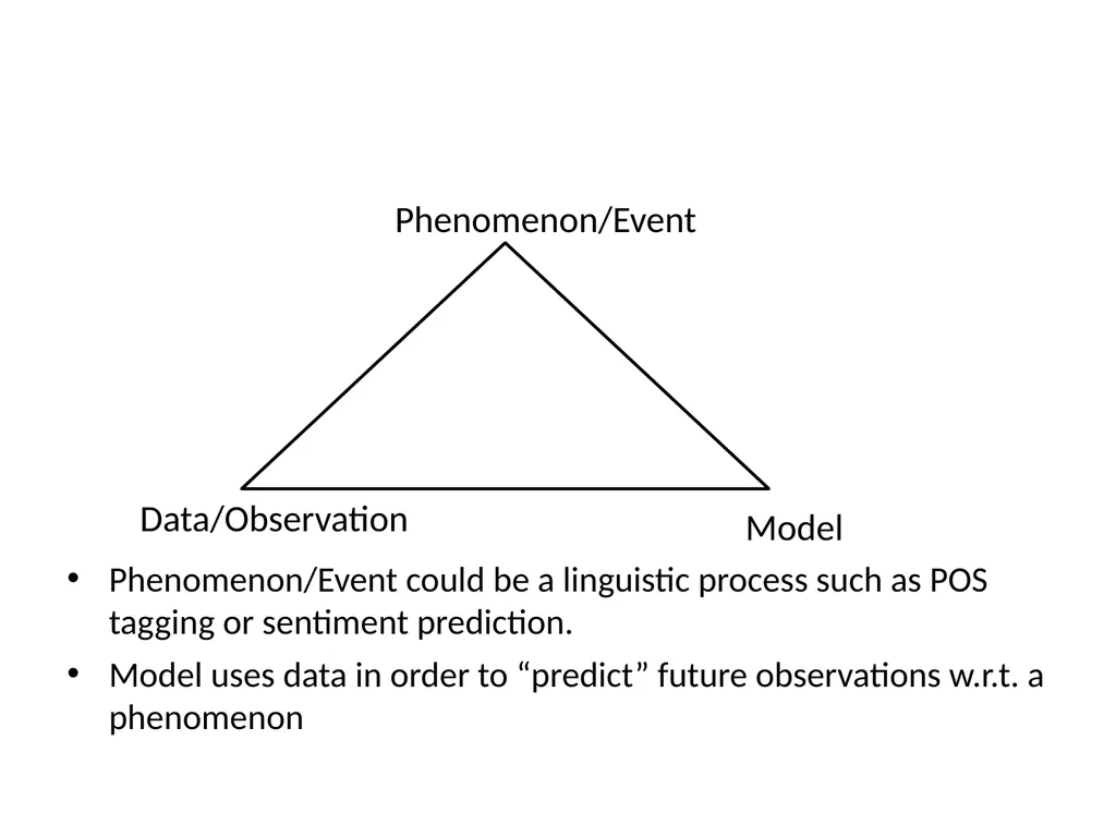
slide2. Phenomenon/Event could be a linguistic process such as POS tagging or sentiment prediction.
Model uses data in order to “predict” future observations w.r.t. a phenomenon Data/Observation Phenomenon/Event Model<br>
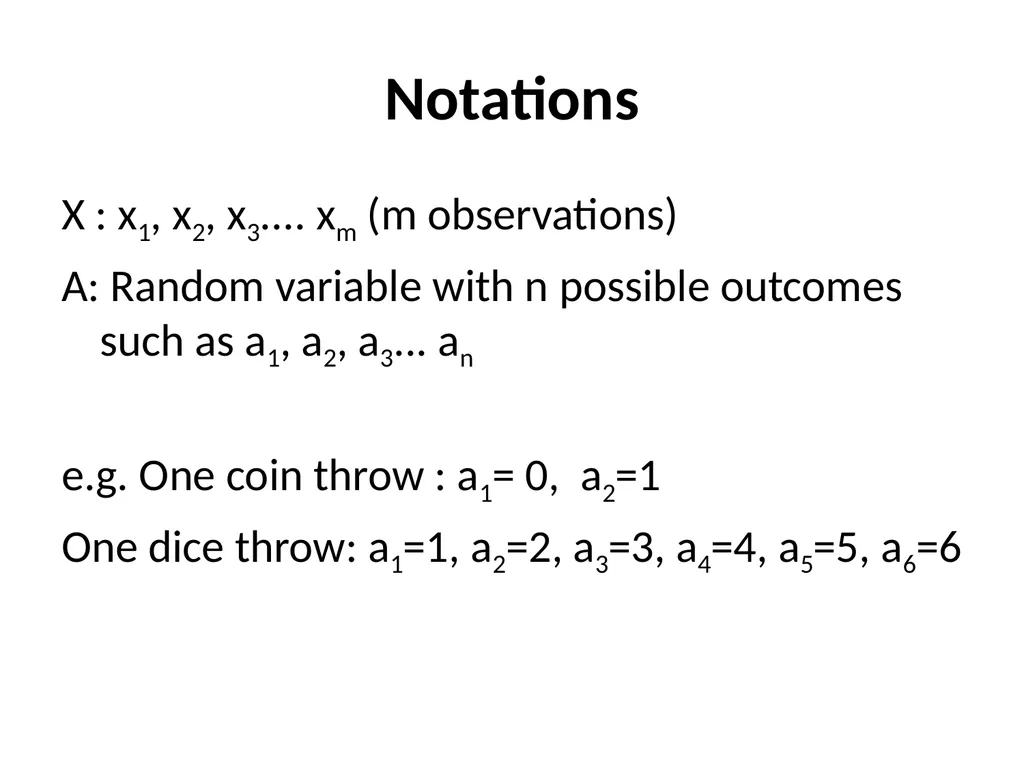
slide3. Notations X : x1, x2, x3.... xm (m observations)
A: Random variable with n possible outcomes such as a1, a2, a3... an

e.g. One coin throw : a1= 0, a2=1
One dice throw: a1=1, a2=2, a3=3, a4=4, a5=5, a6=6<br>
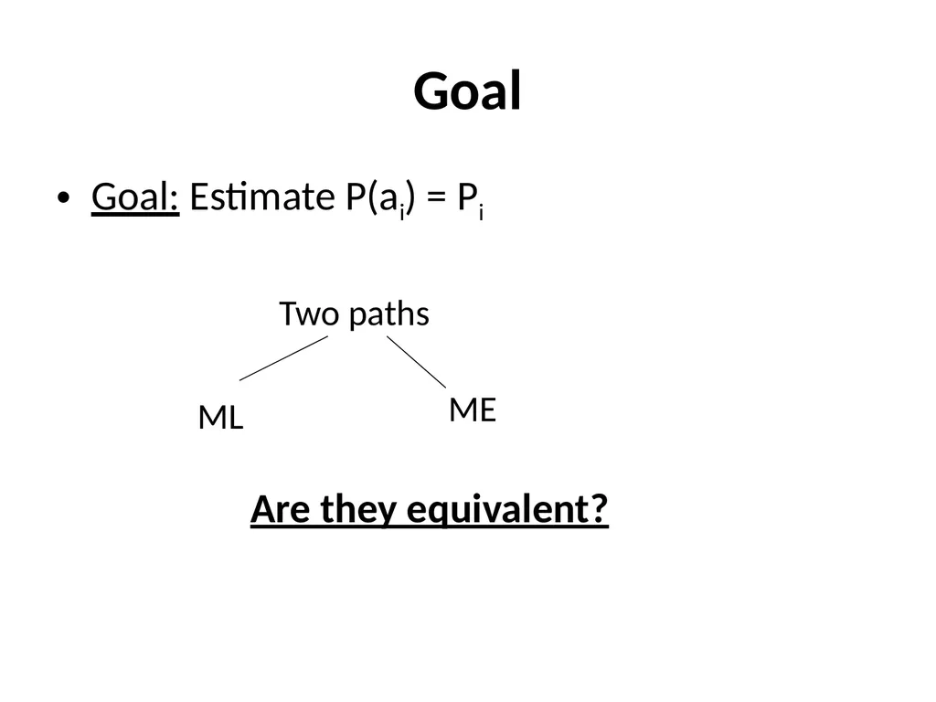
slide4. Goal Goal: Estimate P(ai) = Pi Two paths ML ME Are they equivalent?<br>
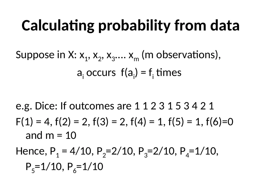
slide5. Calculating probability from data Suppose in X: x1, x2, x3.... xm (m observations),
ai occurs f(ai) = fi times

e.g. Dice: If outcomes are 1 1 2 3 1 5 3 4 2 1
F(1) = 4, f(2) = 2, f(3) = 2, f(4) = 1, f(5) = 1, f(6)=0 and m = 10
Hence, P1 = 4/10, P2=2/10, P3=2/10, P4=1/10, P5=1/10, P6=1/10<br>
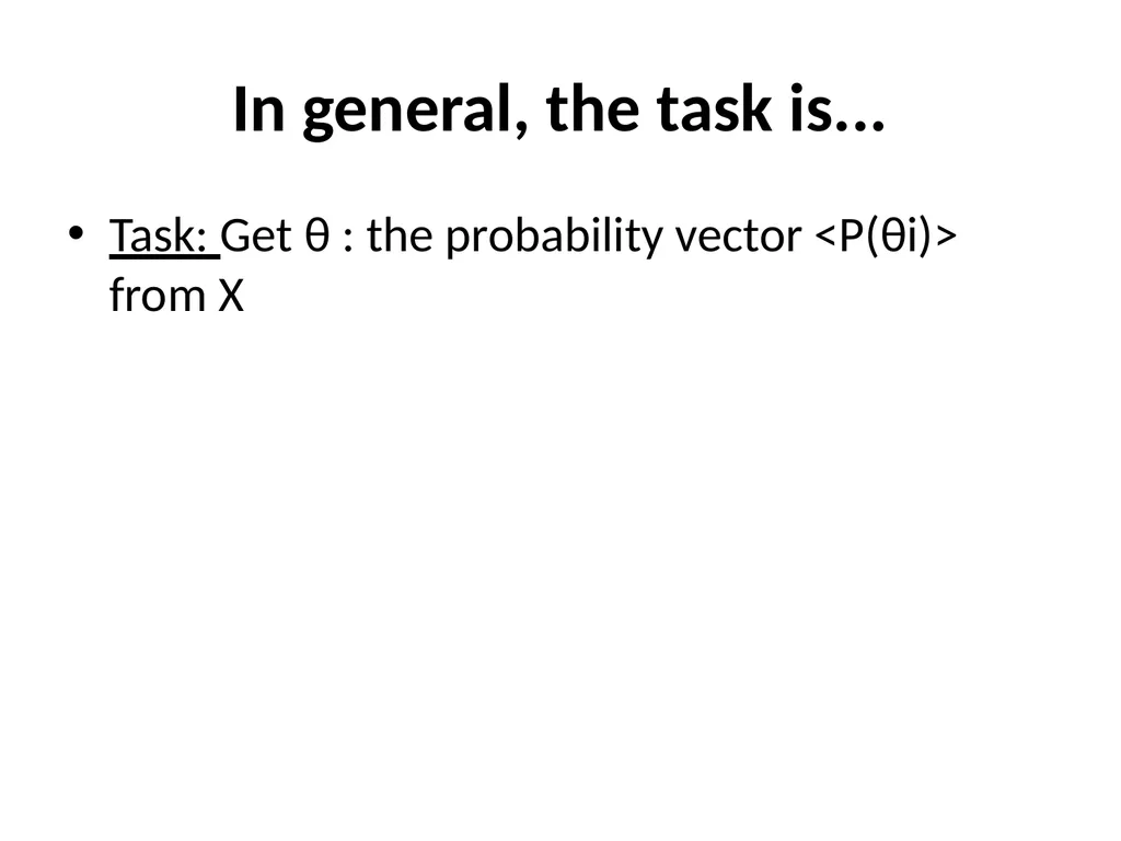
slide6. In general, the task is... Task: Get θ : the probability vector <P(θi)> from X<br>
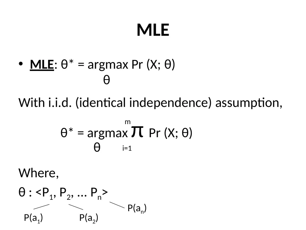
slide7. MLE MLE: θ* = argmax Pr (X; θ)

With i.i.d. (identical independence) assumption,
θ* = argmax π Pr (X; θ)

Where,
θ : <P1, P2, ... Pn> θ θ i=1 m P(a1) P(a2) P(an)<br>
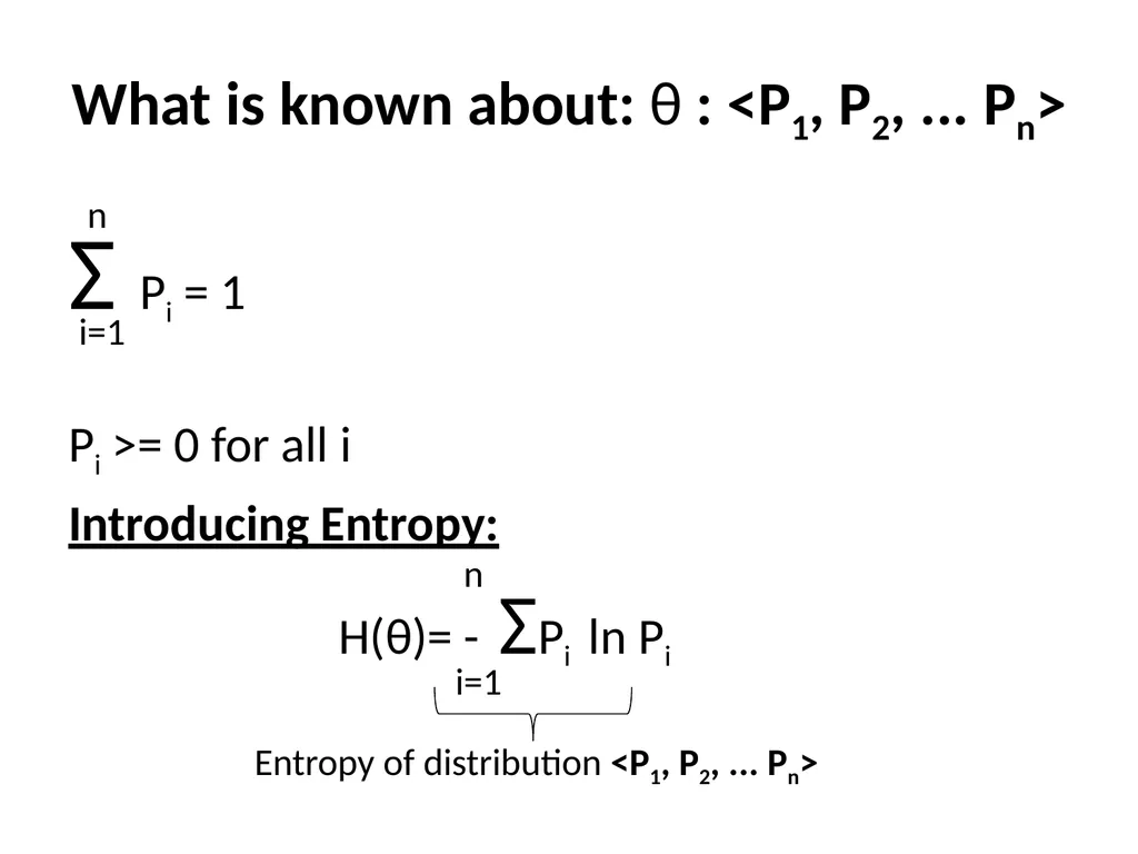
slide8. What is known about: θ : <P1, P2, ... Pn> Σ Pi = 1

Pi >= 0 for all i
Introducing Entropy:
H(θ)= - ΣPi ln Pi i=1 n i=1 n Entropy of distribution <P1, P2, ... Pn><br>
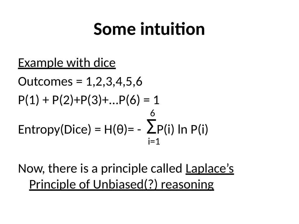
slide9. Some intuition Example with dice
Outcomes = 1,2,3,4,5,6
P(1) + P(2)+P(3)+...P(6) = 1
Entropy(Dice) = H(θ)= - ΣP(i) ln P(i)

Now, there is a principle called Laplace’s Principle of Unbiased(?) reasoning i=1 6<br>
slide10. The best estimate for the dice P(1) = P(2) = ... P(6) = 1/6

We will now prove it assuming:
NO KNOWLEDGE about the dice except that it has six outcomes, each with probability >= 0 and Σ Pi = 1<br>
slide11. What does “best” mean? “BEST” means most consistent with the situation.

“Best” means that these Pi values should be such that they maximize the entropy.<br>
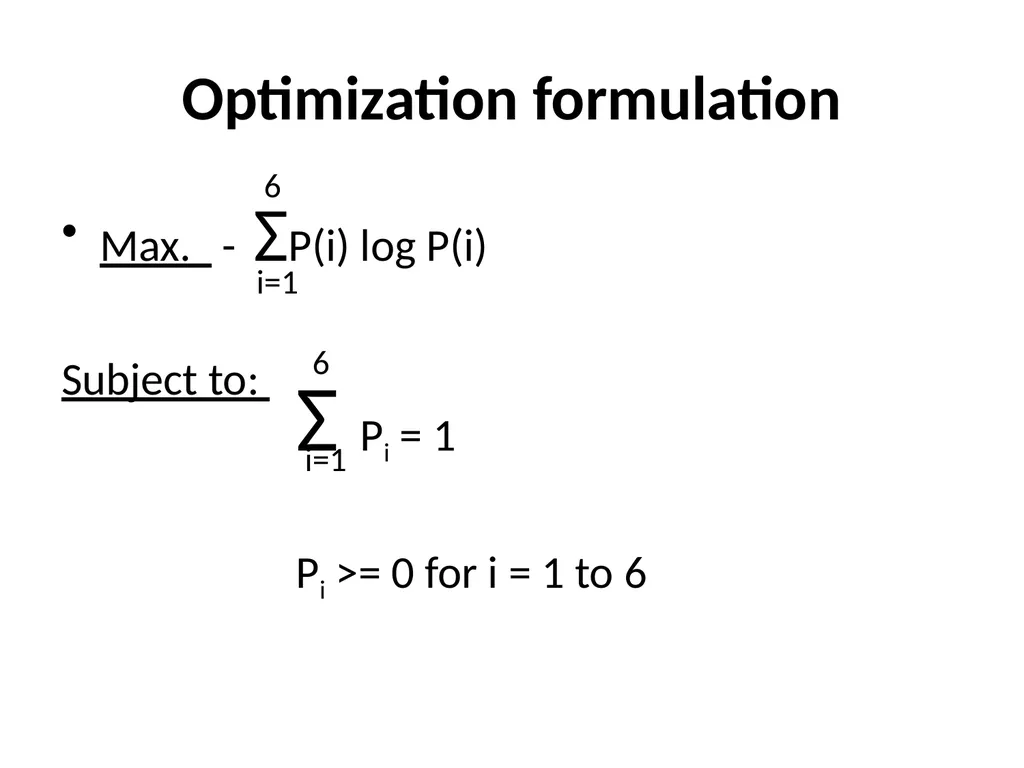
slide12. Optimization formulation Max. - ΣP(i) log P(i)

Subject to: i=1 6 Σ Pi = 1

Pi >= 0 for i = 1 to 6 i=1 6<br>
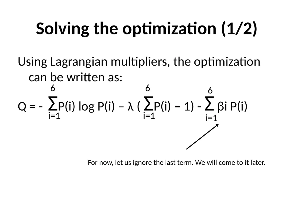
slide13. Solving the optimization (1/2) Using Lagrangian multipliers, the optimization can be written as:
Q = - ΣP(i) log P(i) – λ ( ΣP(i) – 1) - Σ βi P(i) i=1 6 i=1 6 i=1 6 For now, let us ignore the last term. We will come to it later.<br>
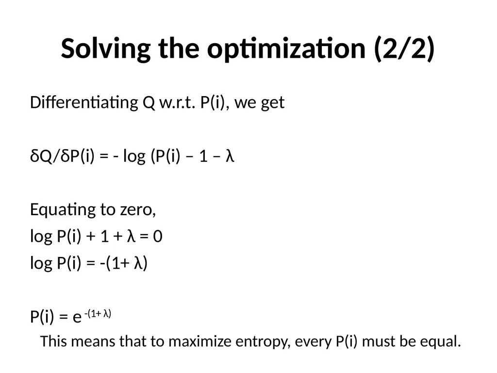
slide14. Solving the optimization (2/2) Differentiating Q w.r.t. P(i), we get

δQ/δP(i) = - log (P(i) – 1 – λ

Equating to zero,
log P(i) + 1 + λ = 0
log P(i) = -(1+ λ)

P(i) = e -(1+ λ) This means that to maximize entropy, every P(i) must be equal.<br>
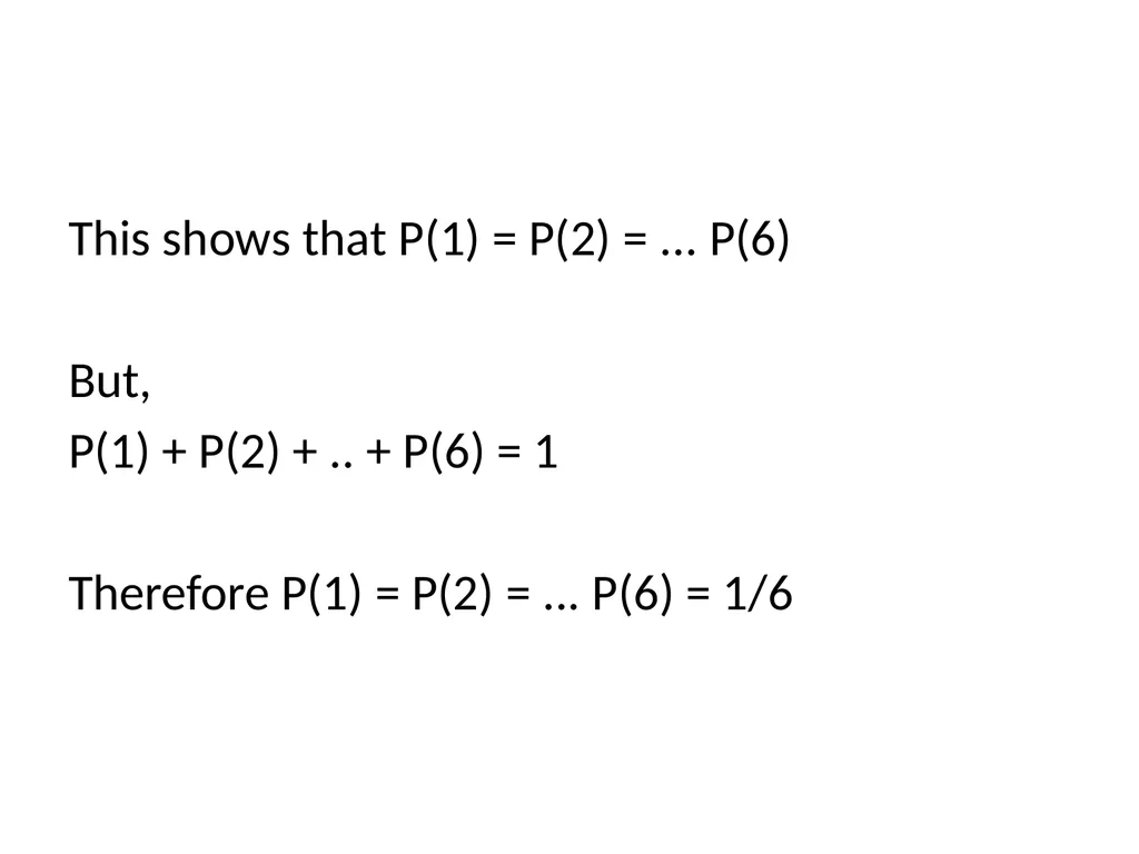
slide15. This shows that P(1) = P(2) = ... P(6)

But,
P(1) + P(2) + .. + P(6) = 1

Therefore P(1) = P(2) = ... P(6) = 1/6<br>
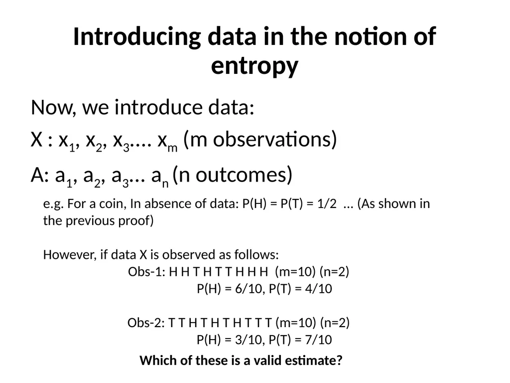
slide16. Introducing data in the notion of entropy Now, we introduce data:
X : x1, x2, x3.... xm (m observations)
A: a1, a2, a3... an (n outcomes) e.g. For a coin, In absence of data: P(H) = P(T) = 1/2 ... (As shown in the previous proof)

However, if data X is observed as follows:
Obs-1: H H T H T T H H H (m=10) (n=2)
P(H) = 6/10, P(T) = 4/10

Obs-2: T T H T H T H T T T (m=10) (n=2)
P(H) = 3/10, P(T) = 7/10 Which of these is a valid estimate?<br>
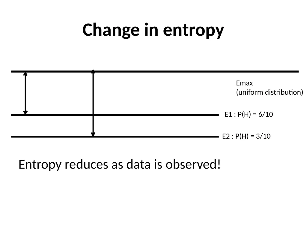
slide17. Change in entropy Entropy reduces as data is observed! Emax
(uniform distribution) E2 : P(H) = 3/10 E1 : P(H) = 6/10<br>
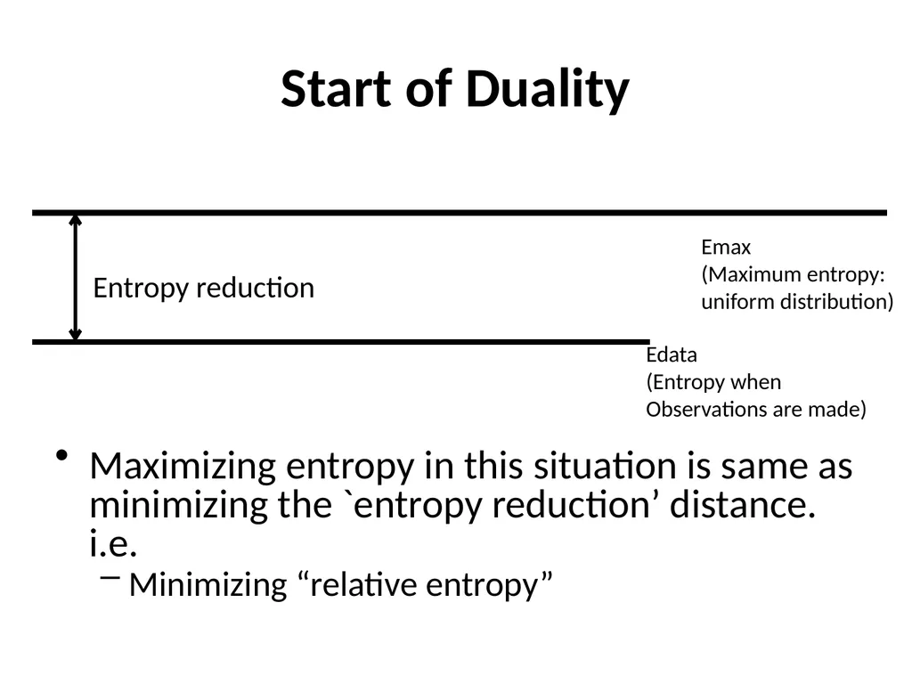
slide18. Start of Duality Maximizing entropy in this situation is same as minimizing the `entropy reduction’ distance. i.e.
Minimizing “relative entropy” Emax
(Maximum entropy:
uniform distribution) Edata
(Entropy when
Observations are made) Entropy reduction<br>
slide19. Concluding remarks Thus, in this discussion of ML-ME duality, we will show that:
MLE minimizes relative entropy distance from uniform distribution.

Question: The entropy corresponds to probability vectors. The distance can be measured by squared distances. WHY relative entropy?<br>
slide20. Maximum Likelihood-Maximum Entropy Duality: Session 2 Pushpak Bhattacharyya

Scribed by Aditya Joshi
Presented in NLP-AI talk on 28th January, 2015<br>
slide21. Recap (1/2) Whatever we can show with MLE, (in most cases), we can through ME as well

Laplace’s unbiased reasoning principle
Make only the most limited assumptions.

We assume data:
X: x1, x2.... Xm m: number of observations
Every xi is the outcome of the values of a random variable<br>
slide22. Recap (2/2) E.g. xi = {1, 2, ...6} for dice.

If no data then by Laplace’s principle, uniform distribution is the best estimate of the probability of each outcome.<br>
slide23. NLP Perspective Probability of mapping of words between parallel sentences.

E.g. The mapping between “blue” and “neela”, and “blue” and “haraa” (wrong translation)

So how can you maintain probabilities of correct mappings based on the corpus?<br>
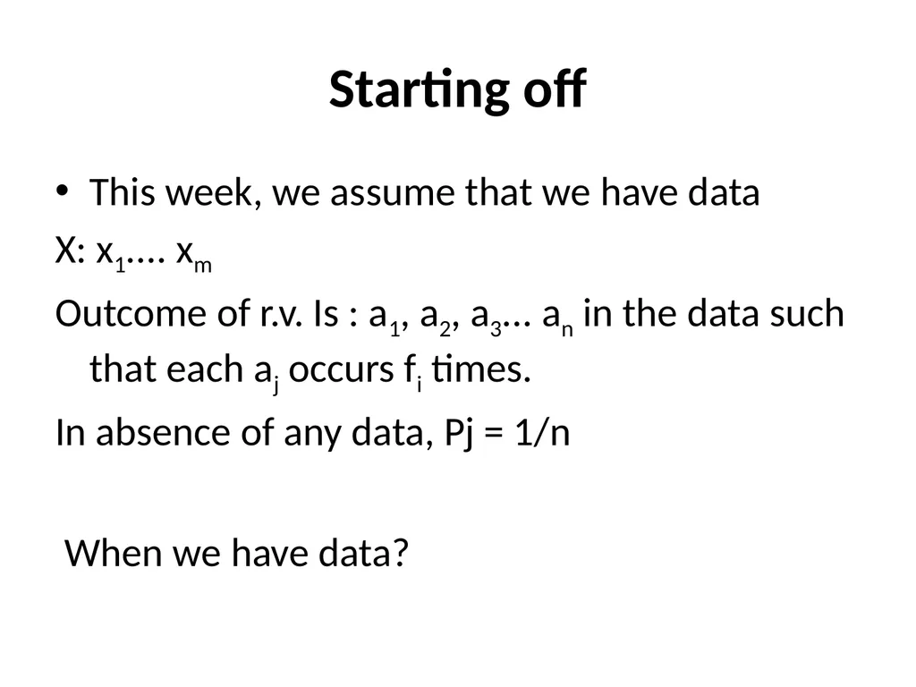
slide24. Starting off This week, we assume that we have data
X: x1.... xm
Outcome of r.v. Is : a1, a2, a3... an in the data such that each aj occurs fi times.
In absence of any data, Pj = 1/n

When we have data?<br>
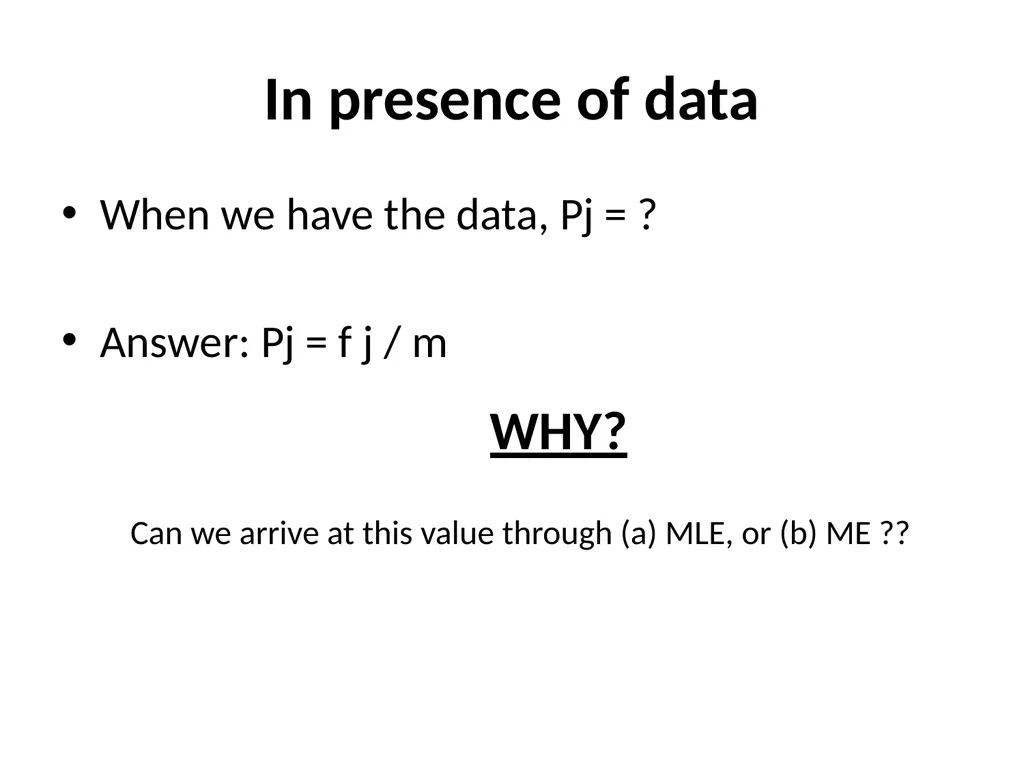
slide25. In presence of data When we have the data, Pj = ?

Answer: Pj = f j / m WHY? Can we arrive at this value through (a) MLE, or (b) ME ??<br>
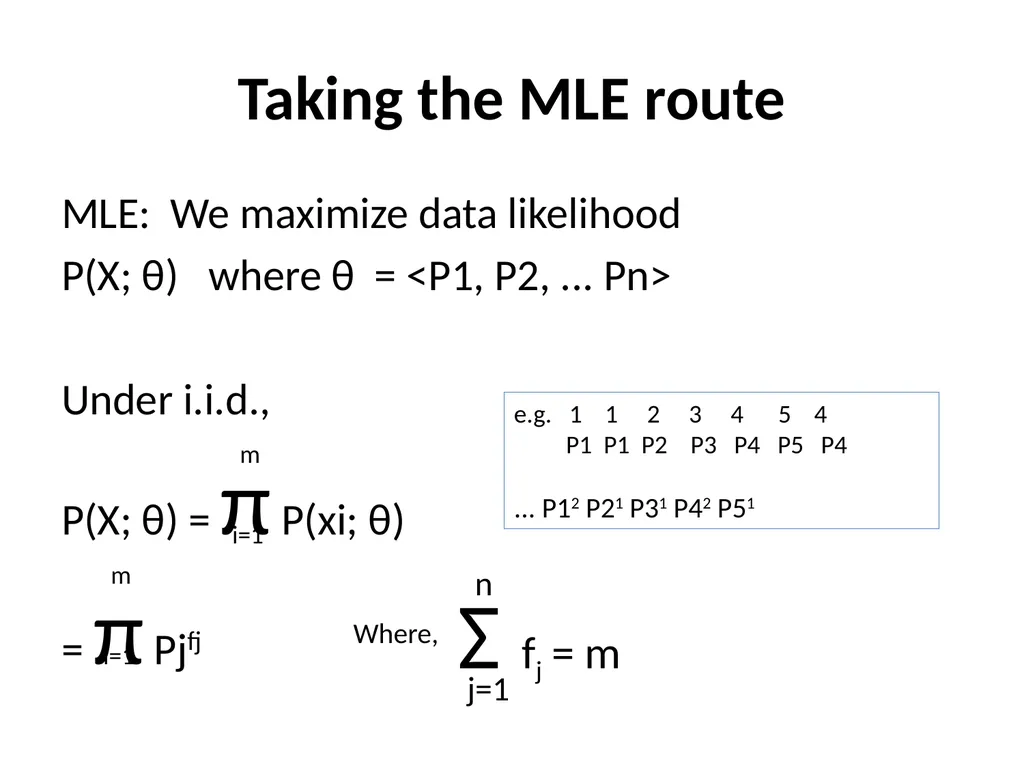
slide26. Taking the MLE route MLE: We maximize data likelihood
P(X; θ) where θ = <P1, P2, ... Pn>

Under i.i.d.,
P(X; θ) = π P(xi; θ)
= π Pjfj i=1 m i=1 m e.g. 1 1 2 3 4 5 4
P1 P1 P2 P3 P4 P5 P4

... P12 P21 P31 P42 P51 Σ fj = m j=1 n Where,<br>
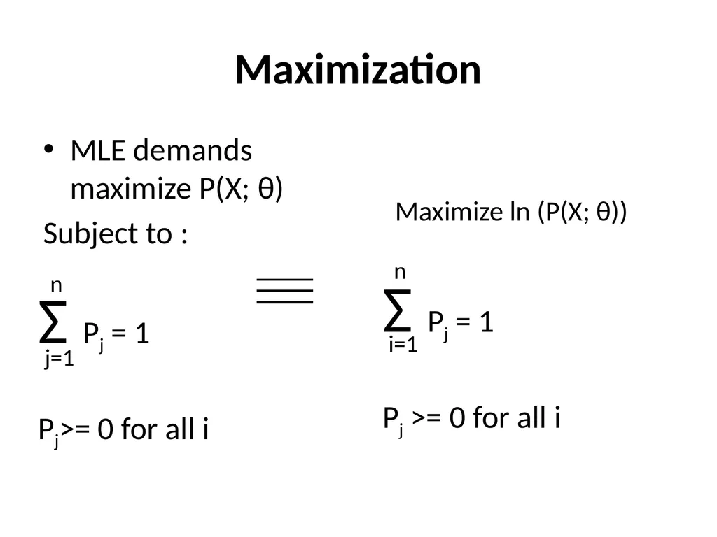
slide27. Maximization MLE demands maximize P(X; θ)
Subject to : Σ Pj = 1

Pj>= 0 for all i j=1 n Maximize ln (P(X; θ)) Σ Pj = 1

Pj >= 0 for all i i=1 n<br>
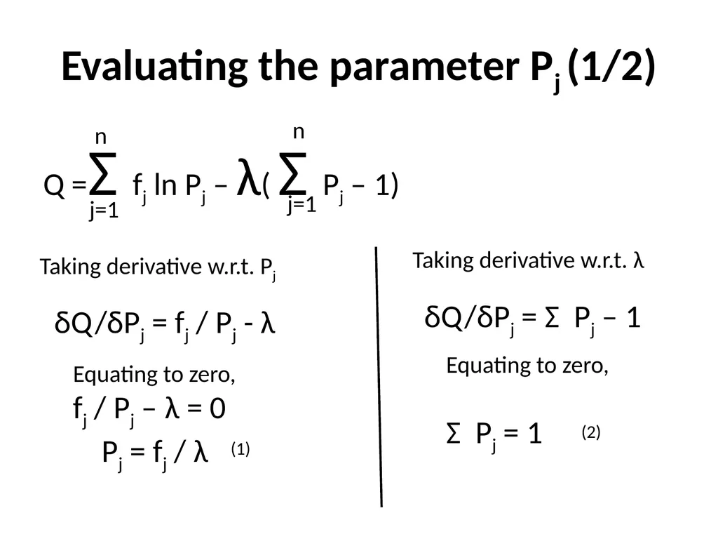
slide28. Evaluating the parameter Pj (1/2) Q =Σ fj ln Pj – λ( Σ Pj – 1) j=1 n j=1 n Taking derivative w.r.t. Pj δQ/δPj = fj / Pj - λ Equating to zero,
fj / Pj – λ = 0
Pj = fj / λ (1) Taking derivative w.r.t. λ δQ/δPj = Σ Pj – 1 Equating to zero,
Σ Pj = 1 (2)<br>
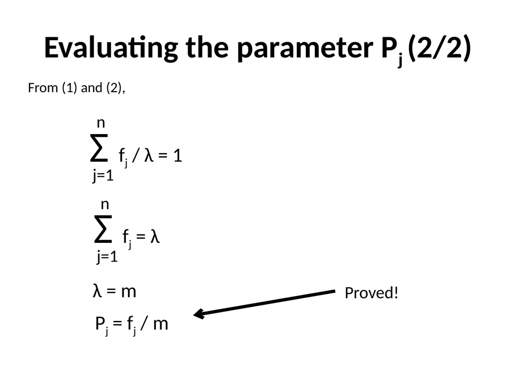
slide29. Evaluating the parameter Pj (2/2) From (1) and (2), Σ fj / λ = 1 j=1 n Σ fj = λ j=1 n λ = m Pj = fj / m Proved!<br>
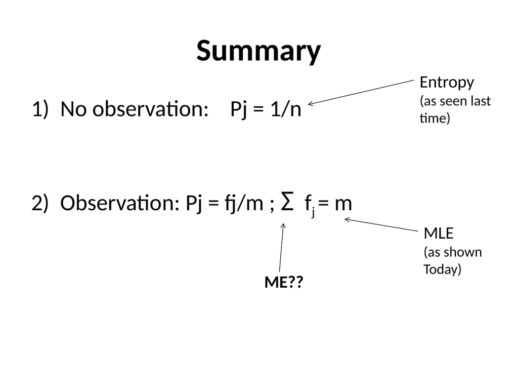
slide30. Summary No observation: Pj = 1/n

Observation: Pj = fj/m ; Σ fj = m Entropy
(as seen last
time) MLE
(as shown
Today) ME??<br>
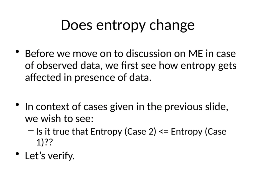
slide31. Does entropy change Before we move on to discussion on ME in case of observed data, we first see how entropy gets affected in presence of data.

In context of cases given in the previous slide, we wish to see:
Is it true that Entropy (Case 2) <= Entropy (Case 1)??
Let’s verify.<br>
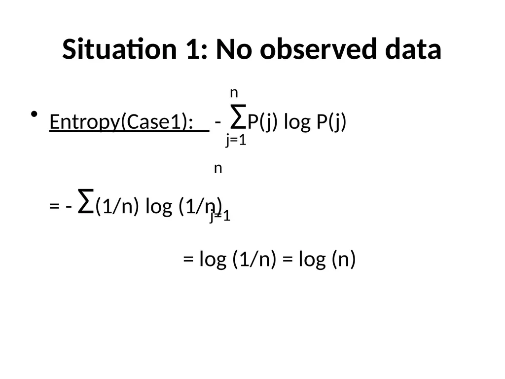
slide32. Situation 1: No observed data Entropy(Case1): - ΣP(j) log P(j)

= - Σ(1/n) log (1/n) j=1 n j=1 n = log (1/n) = log (n)<br>
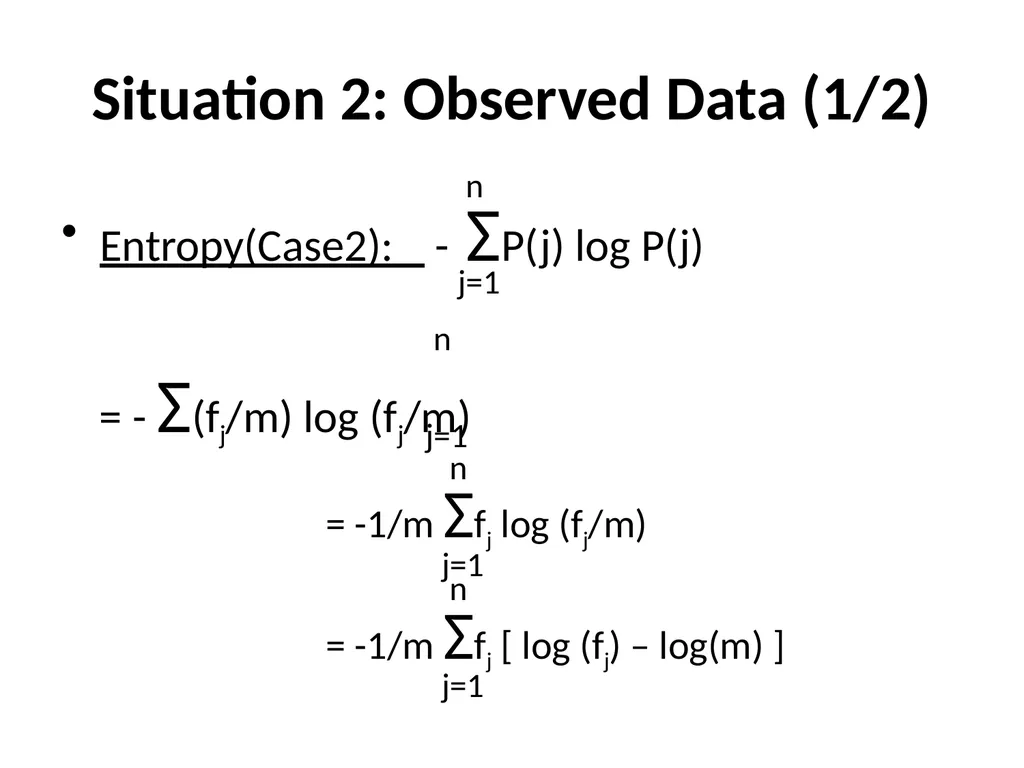
slide33. Situation 2: Observed Data (1/2) Entropy(Case2): - ΣP(j) log P(j)

= - Σ(fj/m) log (fj/m) j=1 n j=1 n = -1/m Σfj log (fj/m) j=1 n = -1/m Σfj [ log (fj) – log(m) ] j=1 n<br>
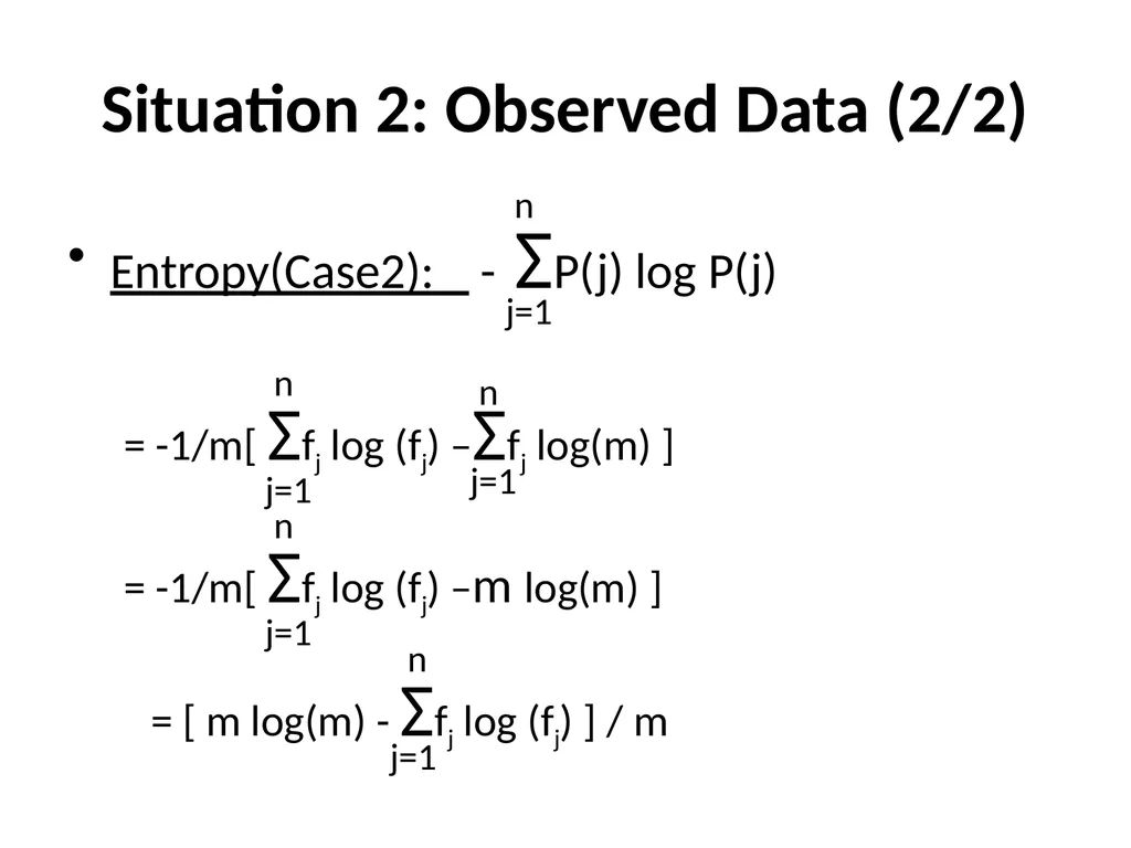
slide34. Situation 2: Observed Data (2/2) Entropy(Case2): - ΣP(j) log P(j) j=1 n = -1/m[ Σfj log (fj) –Σfj log(m) ] j=1 n j=1 n = -1/m[ Σfj log (fj) –m log(m) ] j=1 n = [ m log(m) - Σfj log (fj) ] / m j=1 n<br>
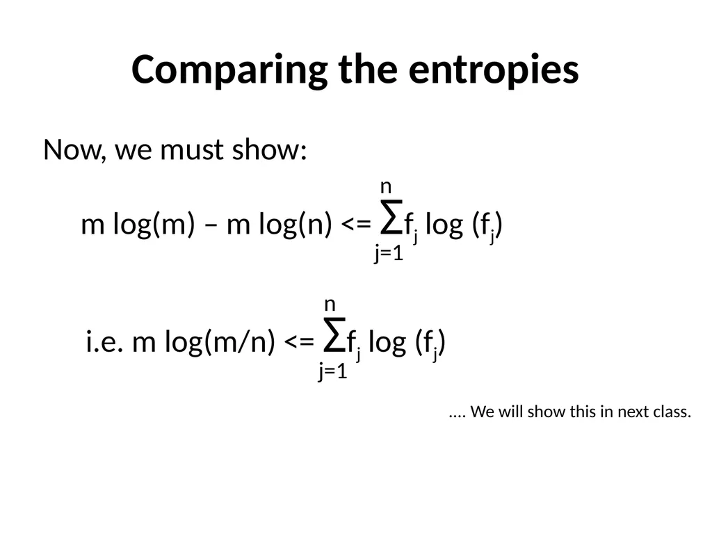
slide35. Comparing the entropies Now, we must show: m log(m) – m log(n) <= Σfj log (fj) j=1 n i.e. m log(m/n) <= Σfj log (fj) j=1 n .... We will show this in next class.<br>
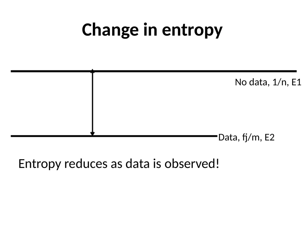
slide36. Change in entropy Entropy reduces as data is observed! No data, 1/n, E1 Data, fj/m, E2<br>
slide37. Concluding remark If you can show that MLE is same as maximum entropy, then MLE-ME duality is shown.<br>
slide38. Maximum Likelihood-Maximum Entropy Duality: Session 3 Pushpak Bhattacharyya

Scribed by Aditya Joshi
Presented in NLP-AI talk on 11th February, 2015<br>
slide39. -Σ fi log Pi

s.t. Σ Pi = 1 & Σ fi = N Recap X1, X2, X3.... XN : Data
A1, A2, A3... AM : Outcomes
Goal: Estimate P(Ai) = Pi In absence of any other information (not even data),
Pi = 1/M

This was obtained using ME

Max. -Σ Pi log Pi

s.t. Σ Pj = 1 i=1 m i=1 m When data is observed,

Pi = fi/N where fi = freq(Ai)
This was obtained using ME
Max. i=1 m i=1 m i=1 m<br>
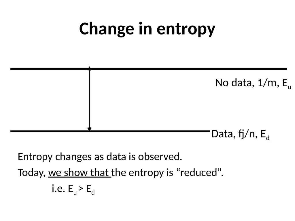
slide40. Change in entropy Entropy changes as data is observed.
Today, we show that the entropy is “reduced”.
i.e. Eu > Ed No data, 1/m, Eu Data, fj/n, Ed<br>
slide41. Today’s goal Today, we will show that the entropy is “reduced”.
i.e. Eu > Ed

Two proofs<br>
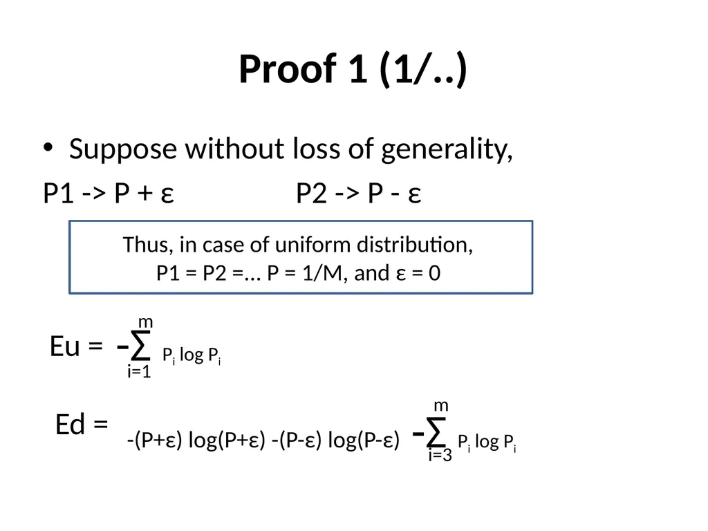
slide42. Proof 1 (1/..) Suppose without loss of generality,
P1 -> P + ε P2 -> P - ε Thus, in case of uniform distribution,
P1 = P2 =... P = 1/M, and ε = 0 -Σ Pi log Pi i=1 m Eu = Ed = -(P+ε) log(P+ε) -(P-ε) log(P-ε) -Σ Pi log Pi i=3 m<br>
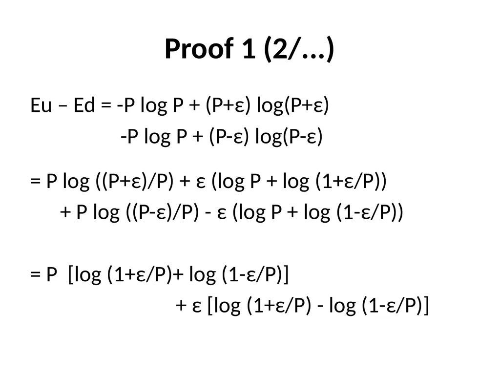
slide43. Proof 1 (2/...) Eu – Ed = -P log P + (P+ε) log(P+ε)
-P log P + (P-ε) log(P-ε)

= P log ((P+ε)/P) + ε (log P + log (1+ε/P))
+ P log ((P-ε)/P) - ε (log P + log (1-ε/P))

= P [log (1+ε/P)+ log (1-ε/P)]
+ ε [log (1+ε/P) - log (1-ε/P)]<br>
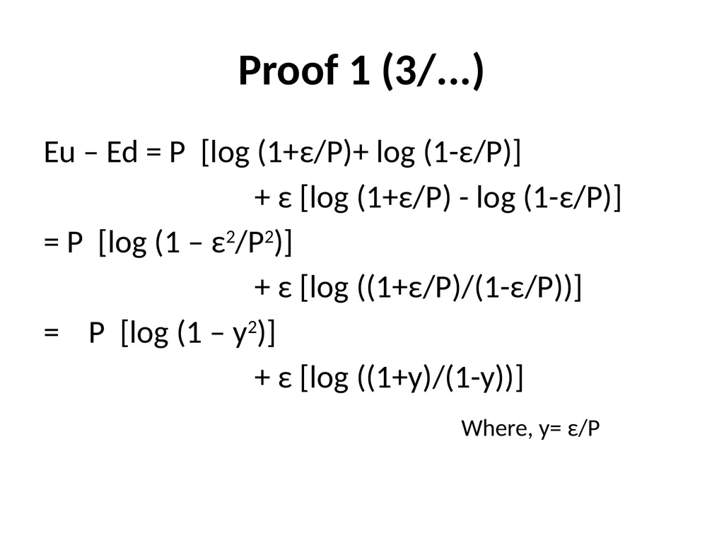
slide44. Proof 1 (3/...) Eu – Ed = P [log (1+ε/P)+ log (1-ε/P)]
+ ε [log (1+ε/P) - log (1-ε/P)]
= P [log (1 – ε2/P2)]
+ ε [log ((1+ε/P)/(1-ε/P))]
= P [log (1 – y2)]
+ ε [log ((1+y)/(1-y))] Where, y= ε/P<br>
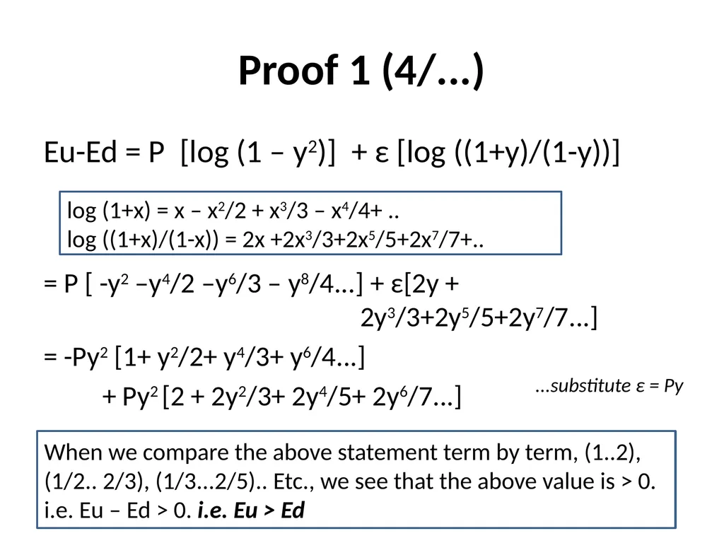
slide45. Proof 1 (4/...) Eu-Ed = P [log (1 – y2)] + ε [log ((1+y)/(1-y))]

= P [ -y2 –y4/2 –y6/3 – y8/4...] + ε[2y + 2y3/3+2y5/5+2y7/7...]
= -Py2 [1+ y2/2+ y4/3+ y6/4...]
+ Py2 [2 + 2y2/3+ 2y4/5+ 2y6/7...] log (1+x) = x – x2/2 + x3/3 – x4/4+ ..
log ((1+x)/(1-x)) = 2x +2x3/3+2x5/5+2x7/7+.. ...substitute ε = Py When we compare the above statement term by term, (1..2), (1/2.. 2/3), (1/3...2/5).. Etc., we see that the above value is > 0. i.e. Eu – Ed > 0. i.e. Eu > Ed<br>
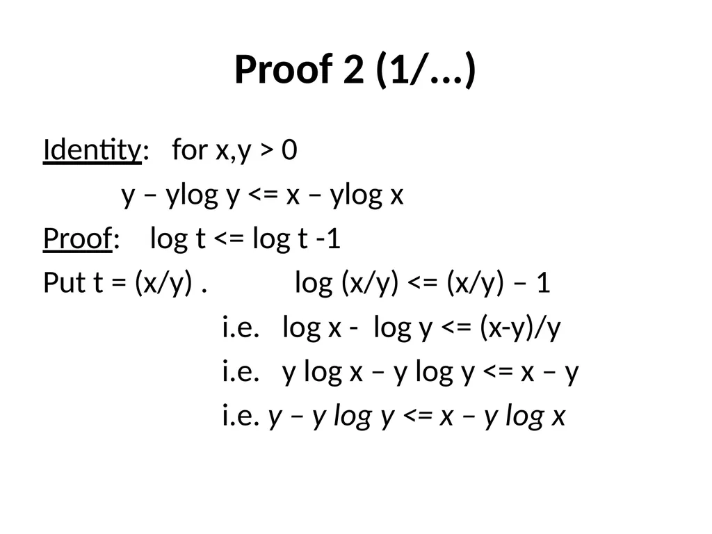
slide46. Proof 2 (1/...) Identity: for x,y > 0
y – ylog y <= x – ylog x
Proof: log t <= log t -1
Put t = (x/y) . log (x/y) <= (x/y) – 1
i.e. log x - log y <= (x-y)/y
i.e. y log x – y log y <= x – y
i.e. y – y log y <= x – y log x<br>
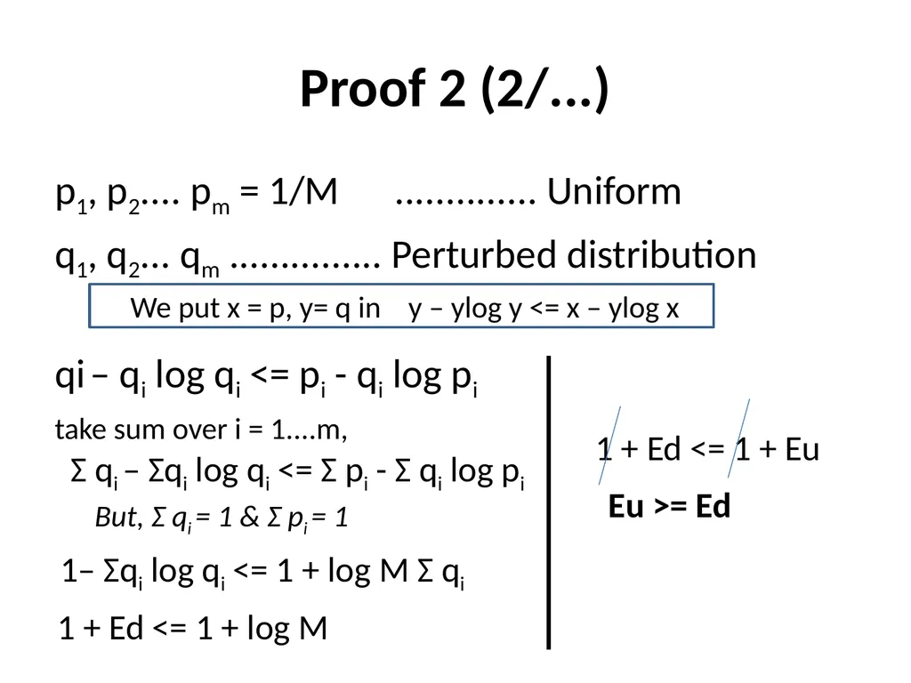
slide47. Proof 2 (2/...) p1, p2.... pm = 1/M .............. Uniform
q1, q2... qm ............... Perturbed distribution

qi – qi log qi <= pi - qi log pi
take sum over i = 1....m, We put x = p, y= q in y – ylog y <= x – ylog x Σ qi – Σqi log qi <= Σ pi - Σ qi log pi But, Σ qi = 1 & Σ pi = 1 1– Σqi log qi <= 1 + log M Σ qi 1 + Ed <= 1 + log M 1 + Ed <= 1 + Eu Eu >= Ed<br>
slide48. Conclusion We showed today that there is a “reduction” in entropy when data is observed.

We showed two proofs: the first is more intuitive but long; the second is simpler.<br>
slide49. Maximum Likelihood-Maximum Entropy Duality: Session 4 Pushpak Bhattacharyya

Scribed by Aditya Joshi
Presented in NLP-AI talk on 25th March, 2015<br>
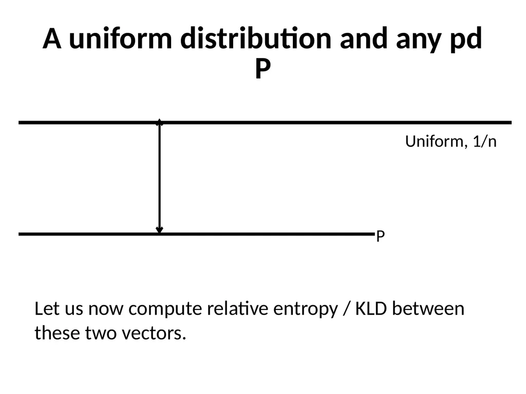
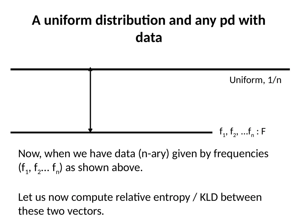
slide50. A uniform distribution and any pd P Uniform, 1/n P Let us now compute relative entropy / KLD between
these two vectors.<br>
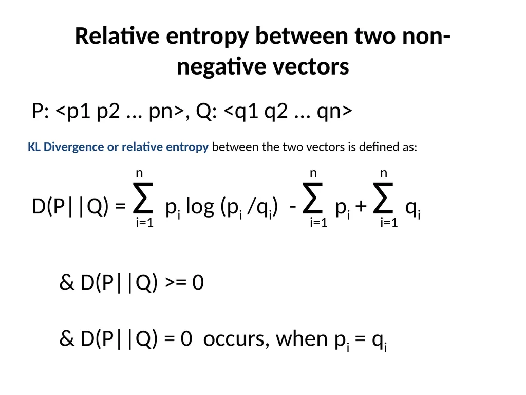
slide51. Relative entropy between two non-negative vectors P: <p1 p2 ... pn>, Q: <q1 q2 ... qn>

D(P||Q) = Σ pi log (pi /qi) - Σ pi + Σ qi i=1 n i=1 n i=1 n KL Divergence or relative entropy between the two vectors is defined as: & D(P||Q) >= 0

& D(P||Q) = 0 occurs, when pi = qi<br>
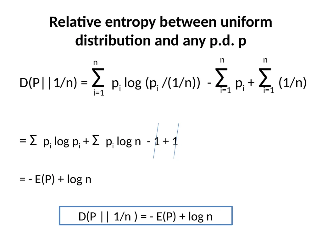
slide52. Relative entropy between uniform distribution and any p.d. p D(P||1/n) = Σ pi log (pi /(1/n)) - Σ pi + Σ (1/n)

= Σ pi log pi + Σ pi log n - 1 + 1

= - E(P) + log n i=1 n i=1 n i=1 n D(P || 1/n ) = - E(P) + log n<br>
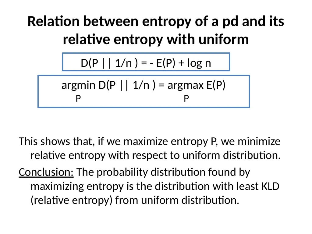
slide53. Relation between entropy of a pd and its relative entropy with uniform This shows that, if we maximize entropy P, we minimize relative entropy with respect to uniform distribution.
Conclusion: The probability distribution found by maximizing entropy is the distribution with least KLD (relative entropy) from uniform distribution. D(P || 1/n ) = - E(P) + log n argmin D(P || 1/n ) = argmax E(P) P P<br>
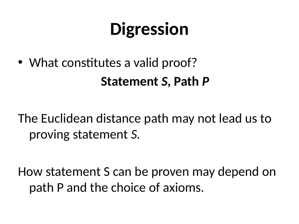
slide54. Digression What constitutes a valid proof?
Statement S, Path P

The Euclidean distance path may not lead us to proving statement S.

How statement S can be proven may depend on path P and the choice of axioms.<br>
slide55. A uniform distribution and any pd with data Uniform, 1/n f1, f2, ...fn : F Now, when we have data (n-ary) given by frequencies (f1, f2... fn) as shown above.

Let us now compute relative entropy / KLD between
these two vectors.<br>
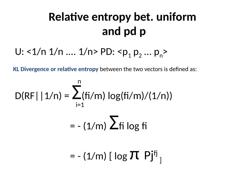
slide56. Relative entropy bet. uniform and pd p U: <1/n 1/n .... 1/n> PD: <p1 p2 ... pn>

D(RF||1/n) = Σ(fi/m) log(fi/m)/(1/n))
= - (1/m) Σfi log fi
= - (1/m) [ log π Pjfj ] i=1 n KL Divergence or relative entropy between the two vectors is defined as:<br>
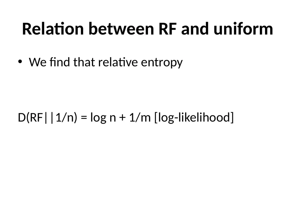
slide57. Relation between RF and uniform We find that relative entropy

D(RF||1/n) = log n + 1/m [log-likelihood]<br>
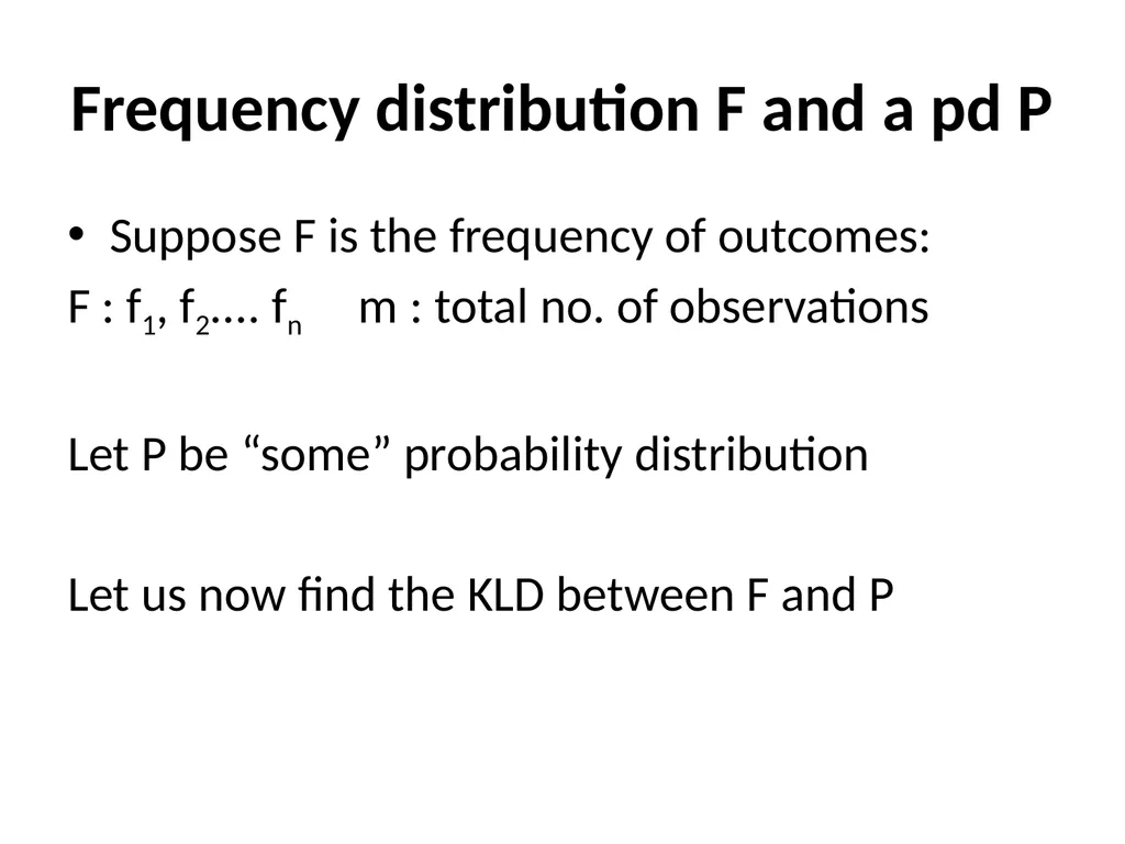
slide58. Frequency distribution F and a pd P Suppose F is the frequency of outcomes:
F : f1, f2.... fn m : total no. of observations

Let P be “some” probability distribution

Let us now find the KLD between F and P<br>
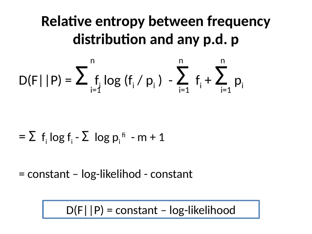
slide59. Relative entropy between frequency distribution and any p.d. p D(F||P) = Σ fi log (fi / pi ) - Σ fi + Σ pi

= Σ fi log fi - Σ log pi fi - m + 1

= constant – log-likelihod - constant i=1 n i=1 n i=1 n D(F||P) = constant – log-likelihood<br>
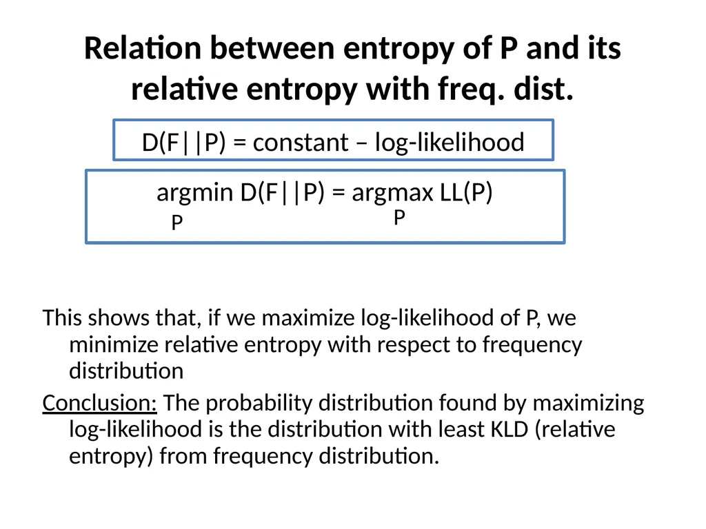
slide60. Relation between entropy of P and its relative entropy with freq. dist. This shows that, if we maximize log-likelihood of P, we minimize relative entropy with respect to frequency distribution
Conclusion: The probability distribution found by maximizing log-likelihood is the distribution with least KLD (relative entropy) from frequency distribution. D(F||P) = constant – log-likelihood argmin D(F||P) = argmax LL(P) P P<br>
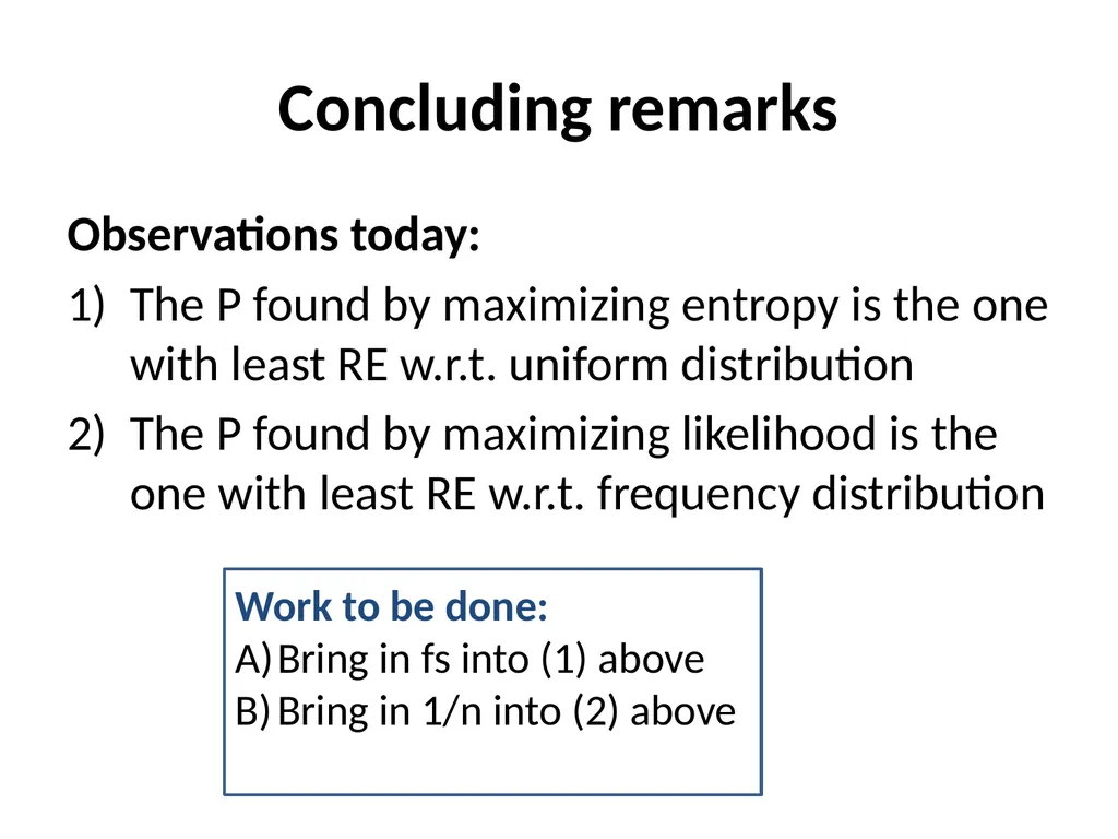
slide61. Concluding remarks Observations today:
The P found by maximizing entropy is the one with least RE w.r.t. uniform distribution
The P found by maximizing likelihood is the one with least RE w.r.t. frequency distribution Work to be done:
Bring in fs into (1) above
Bring in 1/n into (2) above<br>
slide62. Maximum Likelihood-Maximum Entropy Duality: Session 5 Pushpak Bhattacharyya

Scribed by Aditya Joshi
Presented in NLP-AI talk on 17th June, 2015<br>
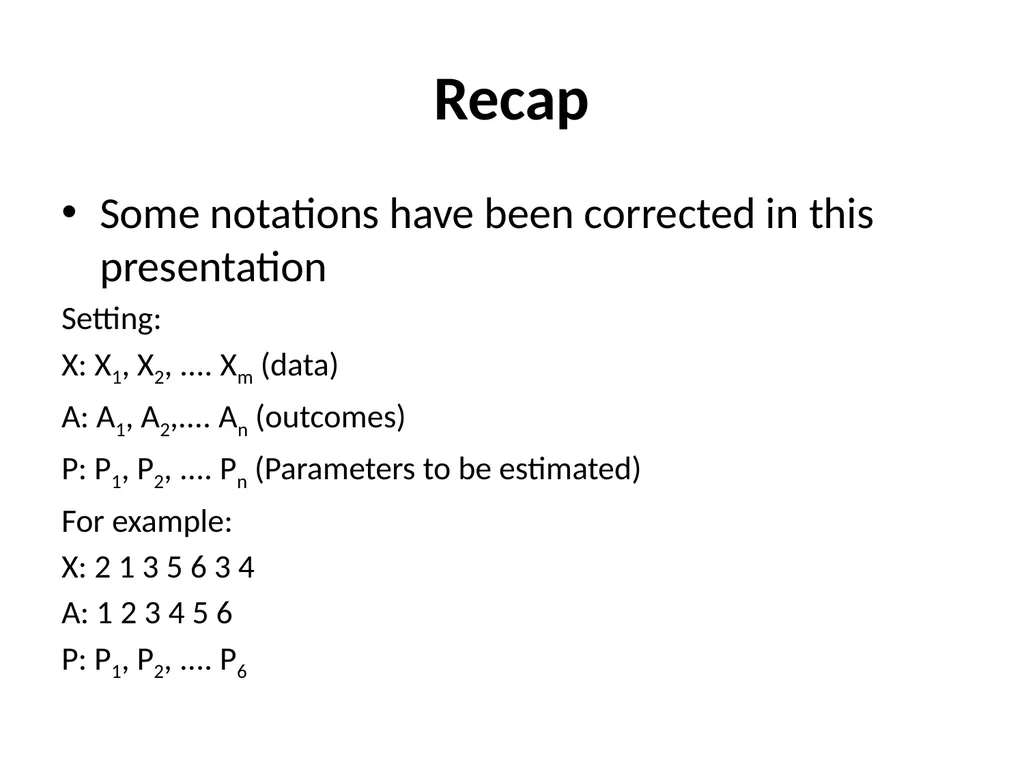
slide63. Recap Some notations have been corrected in this presentation
Setting:
X: X1, X2, .... Xm (data)
A: A1, A2,.... An (outcomes)
P: P1, P2, .... Pn (Parameters to be estimated)
For example:
X: 2 1 3 5 6 3 4
A: 1 2 3 4 5 6
P: P1, P2, .... P6<br>
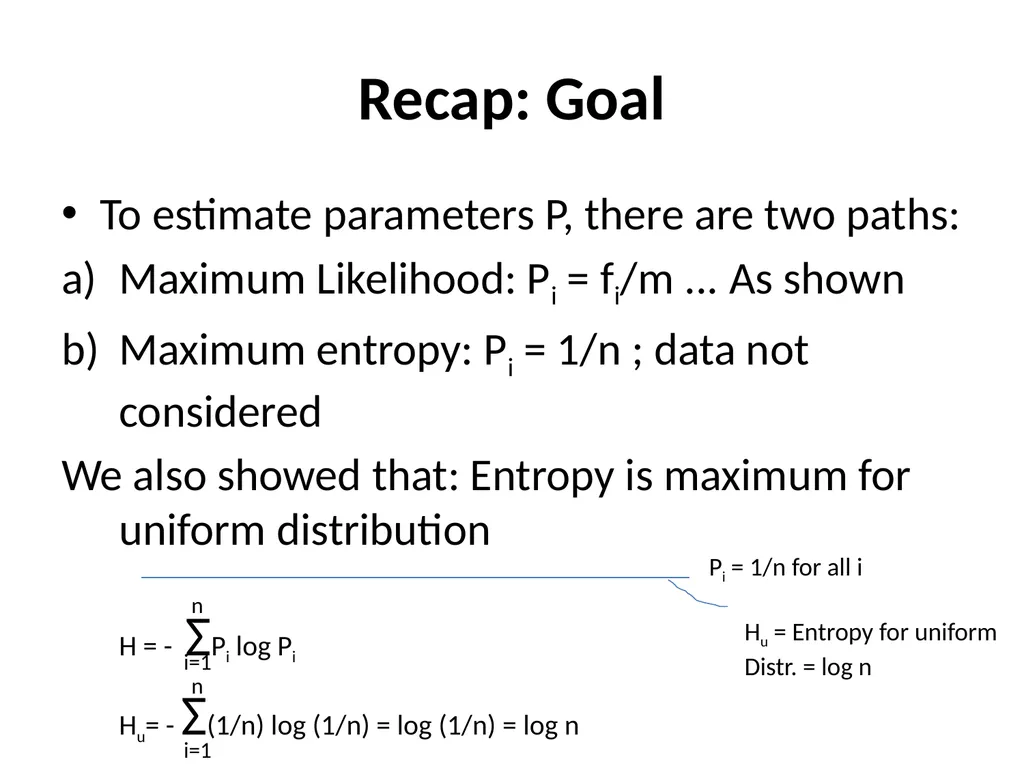
slide64. Recap: Goal To estimate parameters P, there are two paths:
Maximum Likelihood: Pi = fi/m ... As shown
Maximum entropy: Pi = 1/n ; data not considered
We also showed that: Entropy is maximum for uniform distribution Pi = 1/n for all i Hu = Entropy for uniform
Distr. = log n H = - ΣPi log Pi
Hu= - Σ(1/n) log (1/n) = log (1/n) = log n i=1 n j=1 n = log (1/n) = log (n) i=1 n<br>
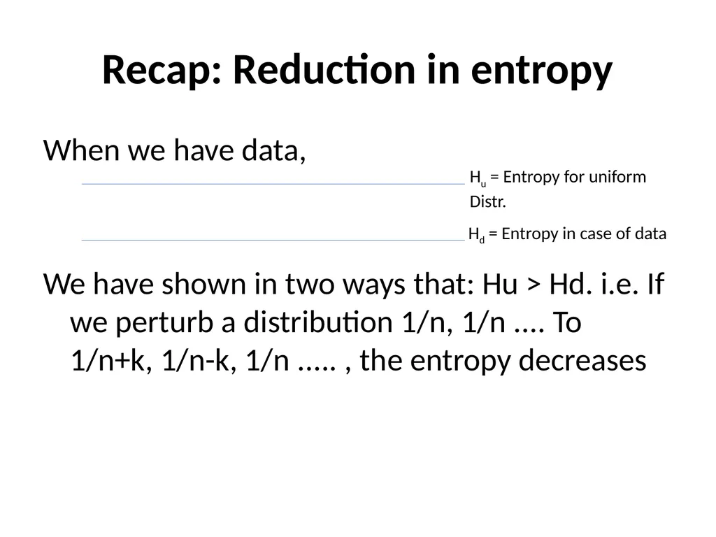
slide65. Recap: Reduction in entropy When we have data,

We have shown in two ways that: Hu > Hd. i.e. If we perturb a distribution 1/n, 1/n .... To 1/n+k, 1/n-k, 1/n ..... , the entropy decreases Hu = Entropy for uniform
Distr. Hd = Entropy in case of data<br>
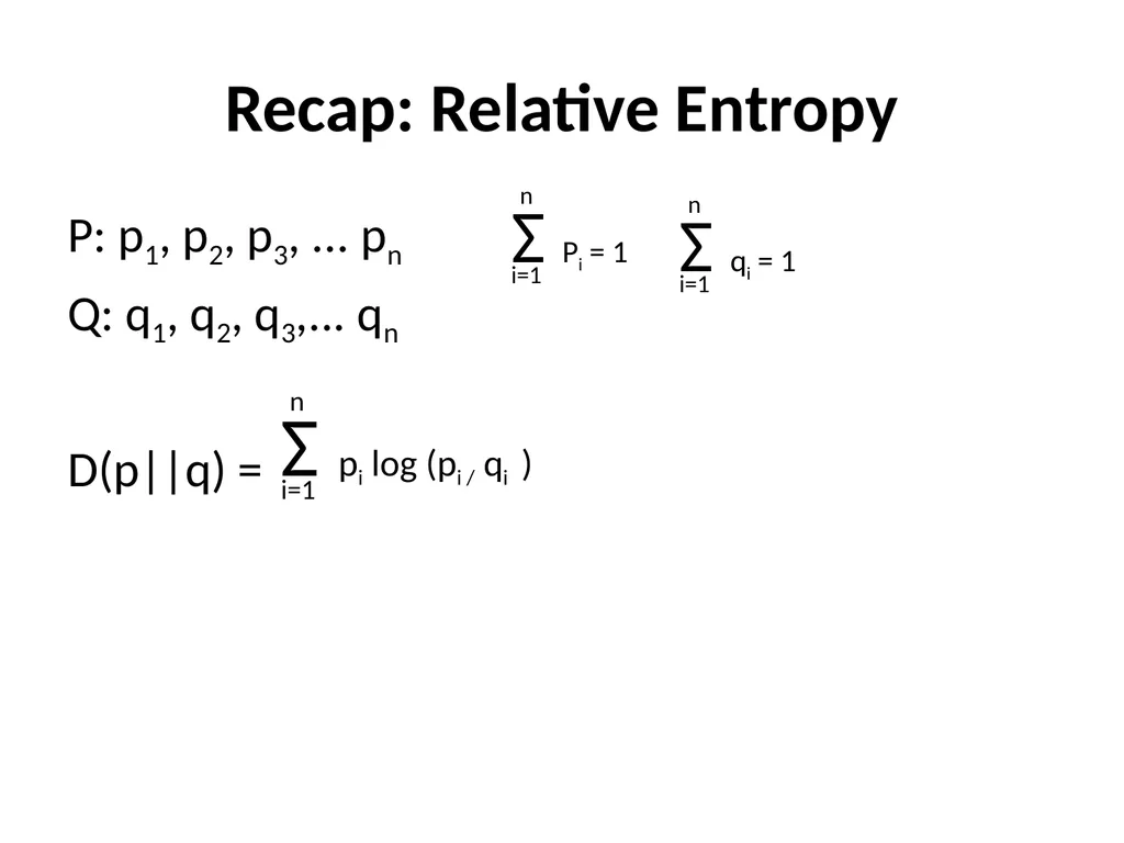
slide66. Recap: Relative Entropy P: p1, p2, p3, ... pn
Q: q1, q2, q3,... qn

D(p||q) = Σ Pi = 1 i=1 n Σ qi = 1 i=1 n Σ pi log (pi / qi ) i=1 n<br>
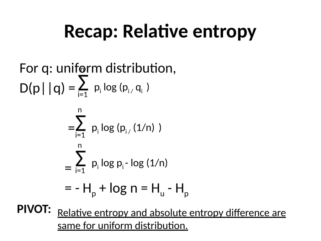
slide67. Recap: Relative entropy For q: uniform distribution,
D(p||q) =

=

=
= - Hp + log n = Hu - Hp Σ pi log (pi / qi ) i=1 n Σ pi log (pi / (1/n) ) i=1 n Σ pi log pi - log (1/n) i=1 n PIVOT: Relative entropy and absolute entropy difference are same for uniform distribution.<br>
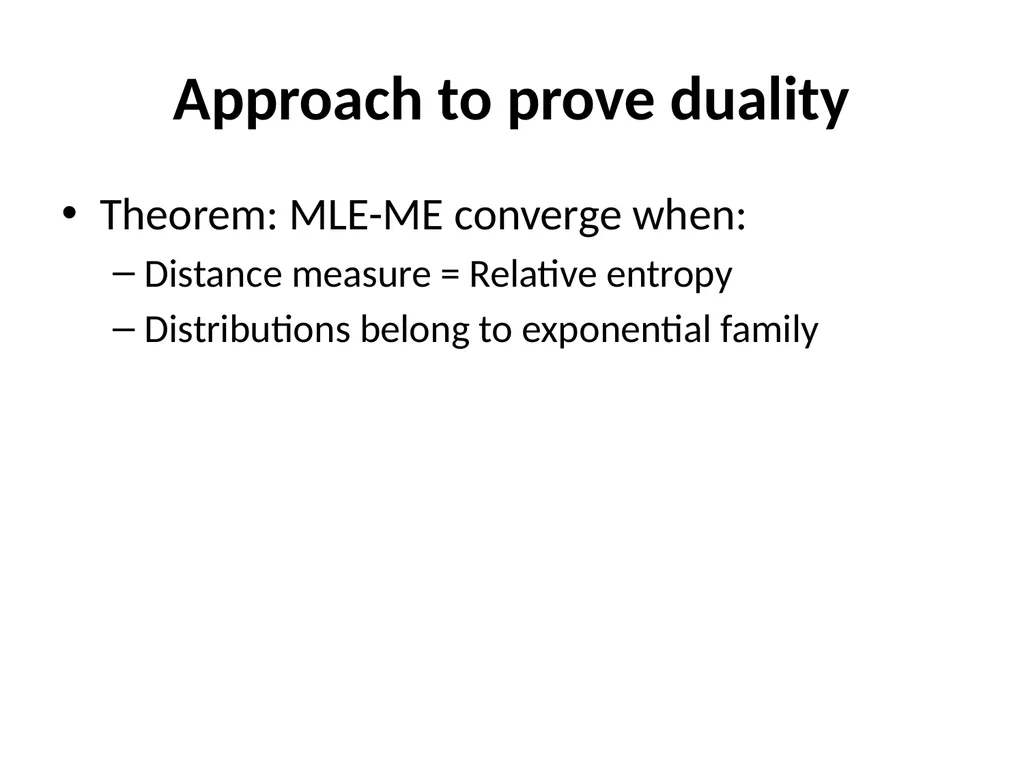
slide68. Approach to prove duality Theorem: MLE-ME converge when:
Distance measure = Relative entropy
Distributions belong to exponential family<br>
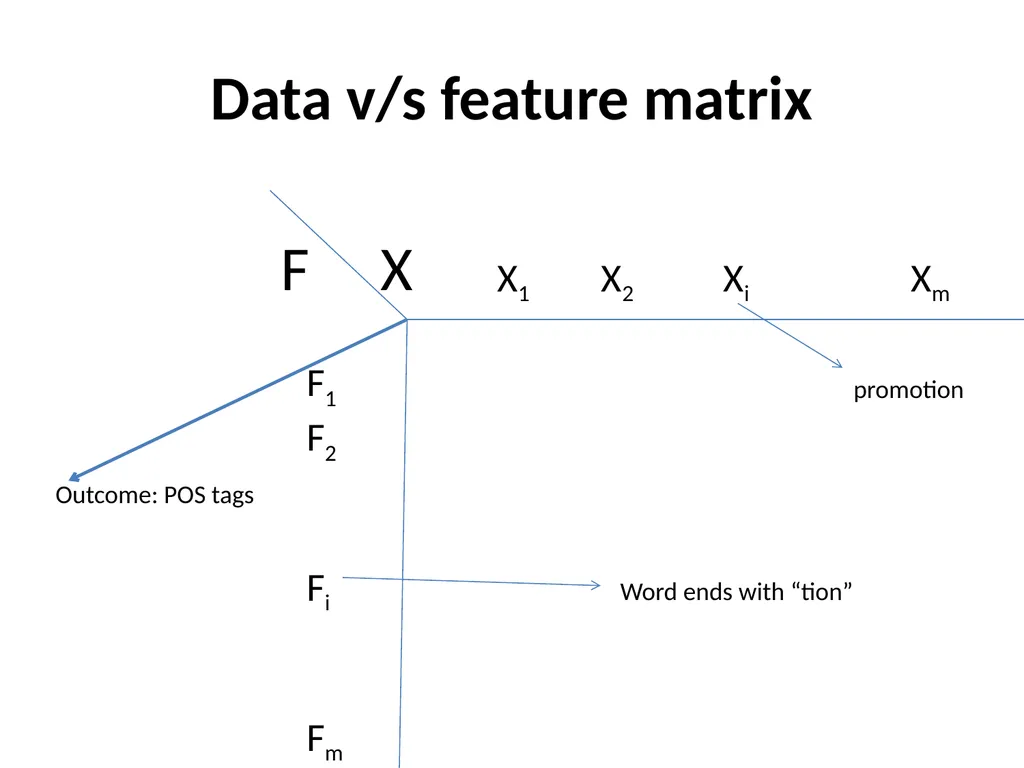
slide69. Data v/s feature matrix X1 X2 Xi Xm F1
F2

Fi

Fm F X promotion Word ends with “tion” Outcome: POS tags<br>
slide70. A note on Outcomes A: A1, A2 ..... An

N is tied to the classification task.

For POS tagging: (Penn Tagset) A: A1, A2 ..... A39<br>
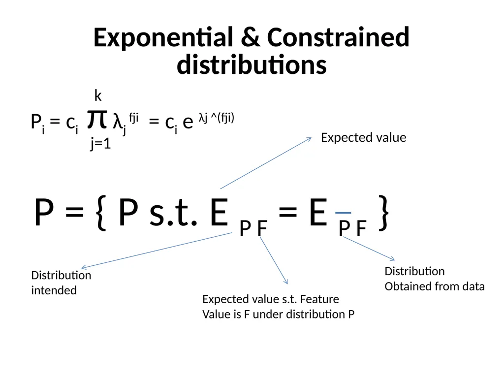
slide71. Exponential & Constrained distributions Pi = ci π λj fji = ci e λj ^(fji) j=1 k P = { P s.t. E P F = E P F } Expected value Distribution
Obtained from data Distribution
intended Expected value s.t. Feature
Value is F under distribution P<br>
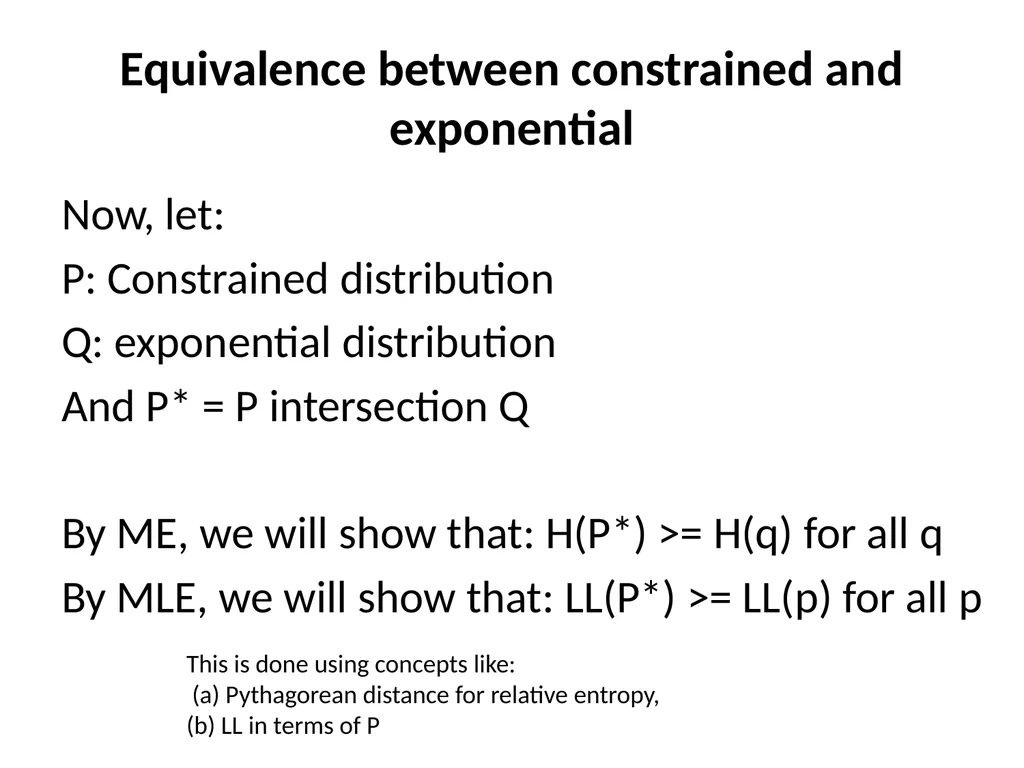
slide72. Equivalence between constrained and exponential Now, let:
P: Constrained distribution
Q: exponential distribution
And P* = P intersection Q

By ME, we will show that: H(P*) >= H(q) for all q
By MLE, we will show that: LL(P*) >= LL(p) for all p This is done using concepts like:
(a) Pythagorean distance for relative entropy,
(b) LL in terms of P<br>
slide73. Maximum Likelihood-Maximum Entropy Duality: Session 6 Pushpak Bhattacharyya

Scribed by Aditya Joshi
Presented in NLP-AI talk on 2nd September, 2015<br>
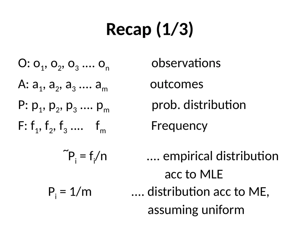
slide74. Recap (1/3) O: o1, o2, o3 .... on observations
A: a1, a2, a3 .... am outcomes
P: p1, p2, p3 .... pm prob. distribution
F: f1, f2, f3 .... fm Frequency Pi = fi/n .... empirical distribution
acc to MLE ~ Pi = 1/m .... distribution acc to ME,
assuming uniform<br>
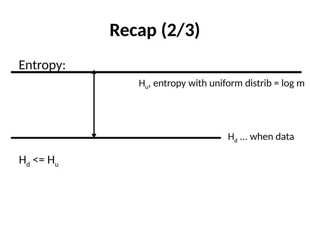
slide75. Recap (2/3) Entropy: Hu, entropy with uniform distrib = log m Hd ... when data Hd <= Hu<br>
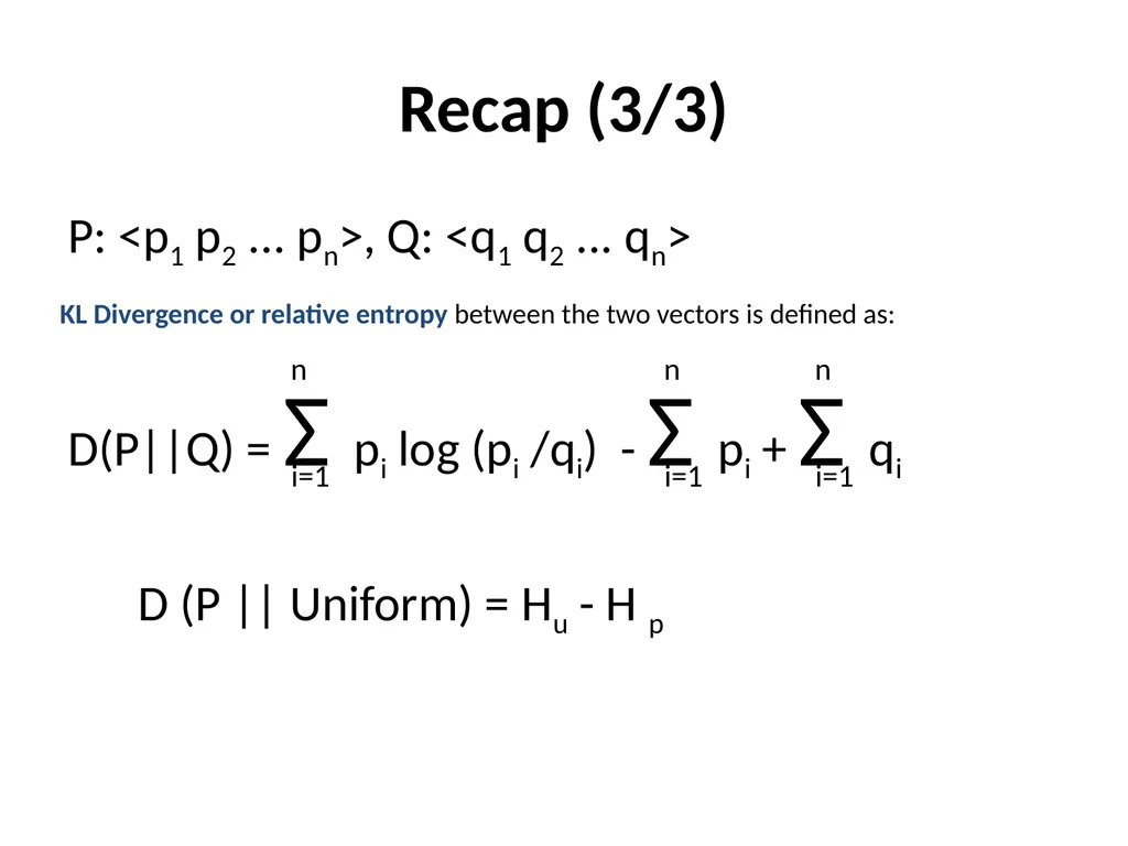
slide76. Recap (3/3) P: <p1 p2 ... pn>, Q: <q1 q2 ... qn>

D(P||Q) = Σ pi log (pi /qi) - Σ pi + Σ qi i=1 n i=1 n i=1 n KL Divergence or relative entropy between the two vectors is defined as: D (P || Uniform) = Hu - H p<br>
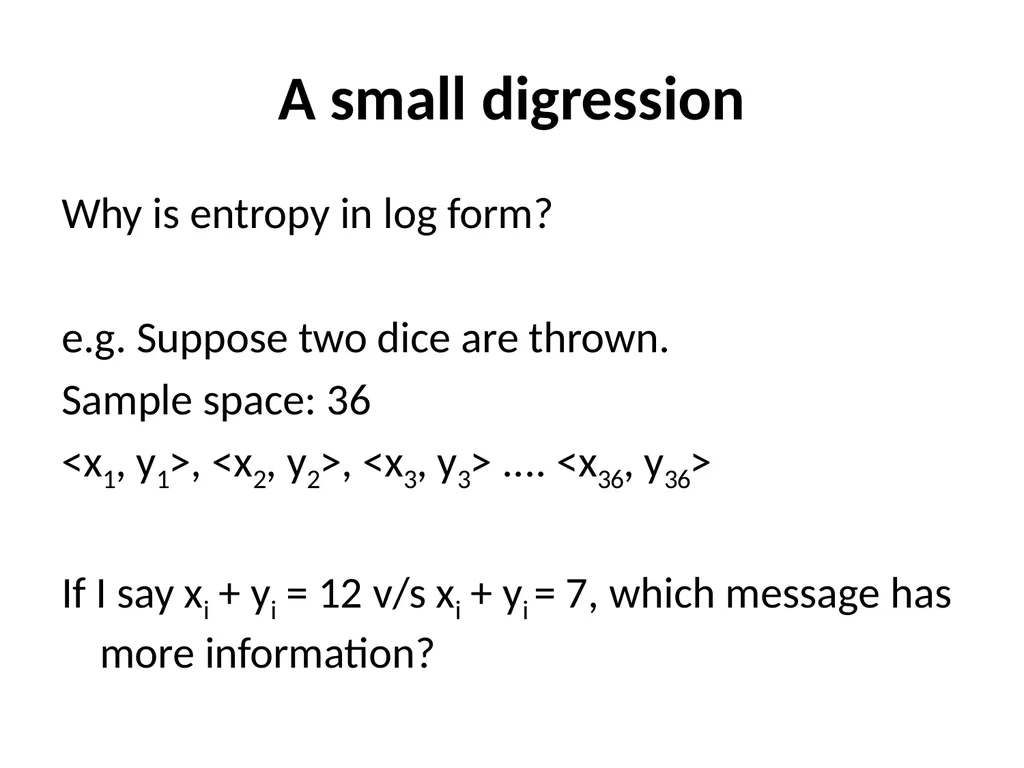
slide77. A small digression Why is entropy in log form?

e.g. Suppose two dice are thrown.
Sample space: 36
<x1, y1>, <x2, y2>, <x3, y3> .... <x36, y36>

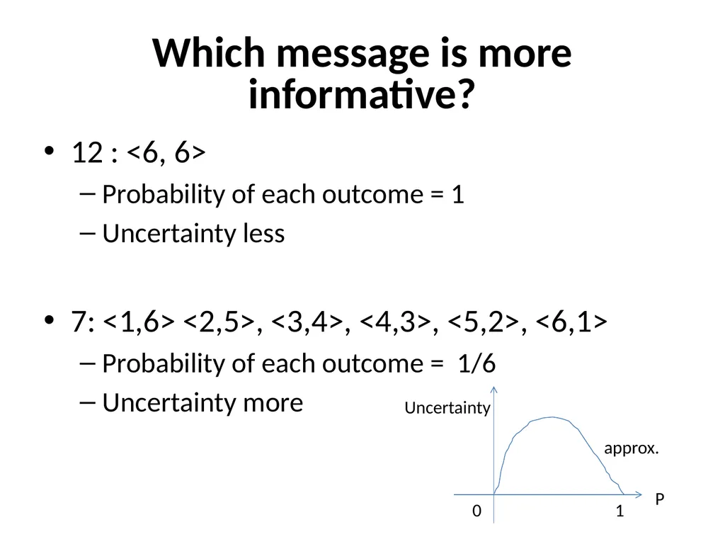
If I say xi + yi = 12 v/s xi + yi = 7, which message has more information?<br>
slide78. Which message is more informative? 12 : <6, 6>
Probability of each outcome = 1
Uncertainty less

7: <1,6> <2,5>, <3,4>, <4,3>, <5,2>, <6,1>
Probability of each outcome = 1/6
Uncertainty more 0 1 P Uncertainty approx.<br>
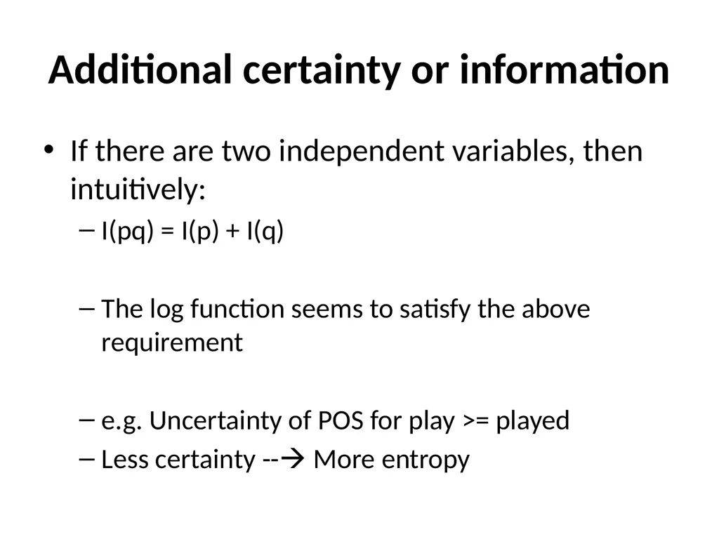
slide79. Additional certainty or information If there are two independent variables, then intuitively:
I(pq) = I(p) + I(q)

The log function seems to satisfy the above requirement

e.g. Uncertainty of POS for play >= played
Less certainty -- More entropy<br>
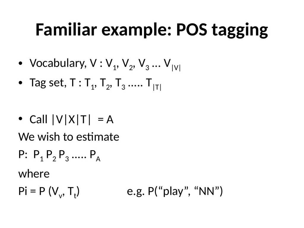
slide80. Familiar example: POS tagging Vocabulary, V : V1, V2, V3 ... V|V|
Tag set, T : T1, T2, T3 ..... T|T|

Call |V|X|T| = A
We wish to estimate
P: P1 P2 P3 ..... PA
where
Pi = P (Vv, Tt) e.g. P(“play”, “NN”)<br>
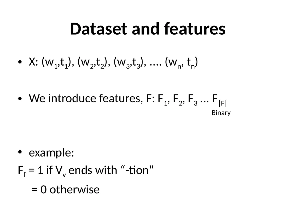
slide81. Dataset and features X: (w1,t1), (w2,t2), (w3,t3), .... (wn, tn)

We introduce features, F: F1, F2, F3 ... F|F|

example:
Ff = 1 if Vv ends with “-tion”
= 0 otherwise Binary<br>
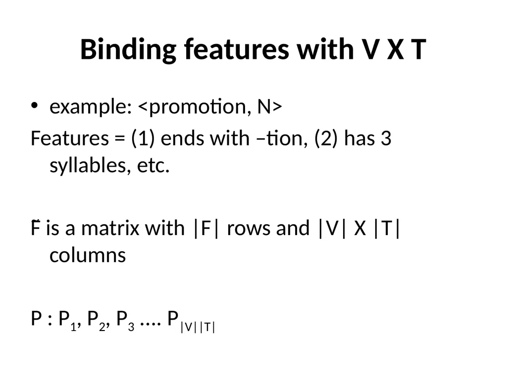
slide82. Binding features with V X T example: <promotion, N>
Features = (1) ends with –tion, (2) has 3 syllables, etc.

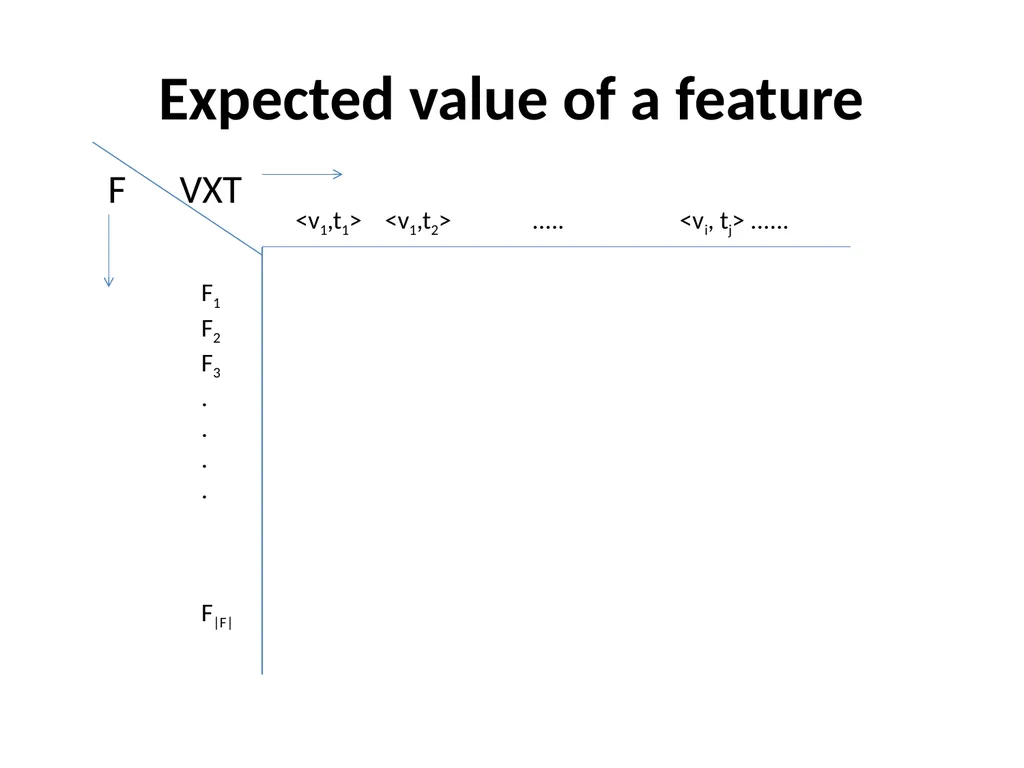
F is a matrix with |F| rows and |V| X |T| columns

P : P1, P2, P3 .... P|V||T| ~<br>
slide83. Expected value of a feature F VXT <v1,t1> <v1,t2> ..... <vi, tj> ...... F1
F2
F3
.
.
.
.

F|F|<br>
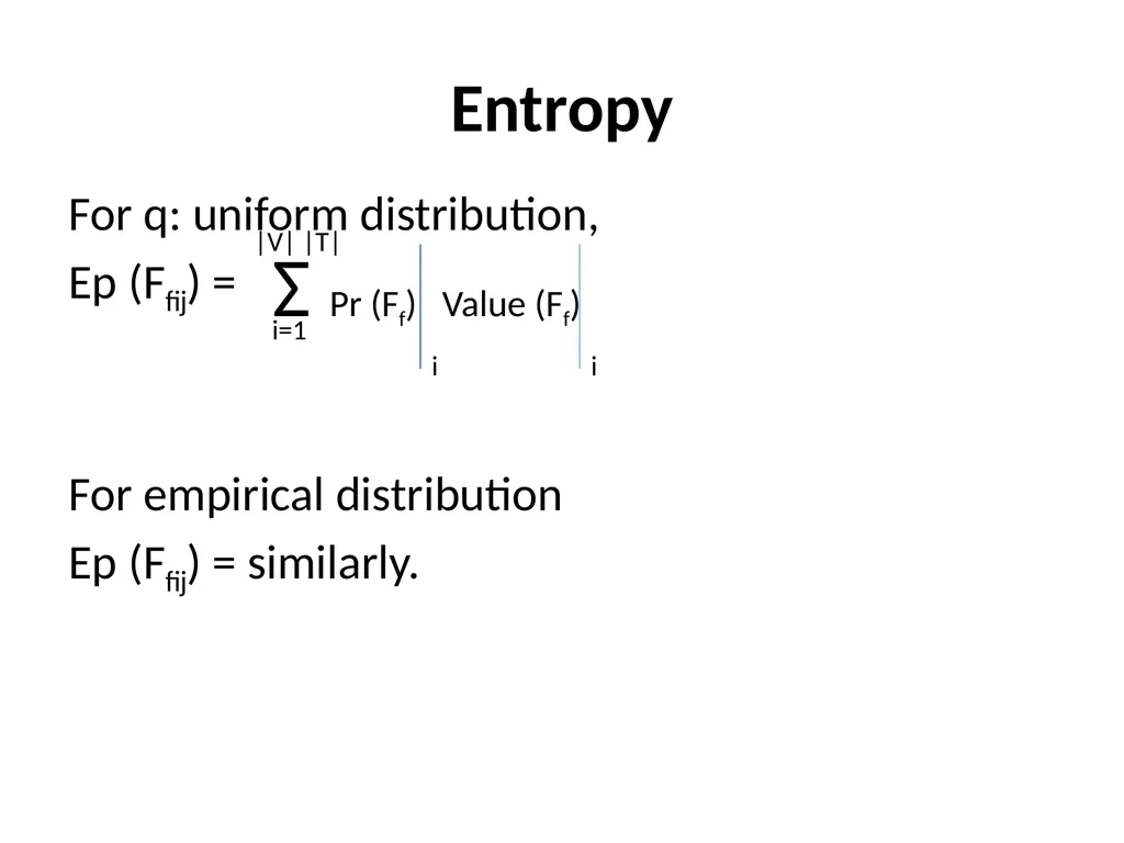
slide84. Entropy For q: uniform distribution,
Ep (Ffij) =


For empirical distribution
Ep (Ffij) = similarly. Σ Pr (Ff) Value (Ff) i=1 |V| |T| i i<br>
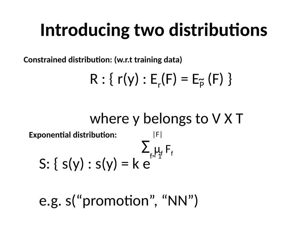
slide85. Introducing two distributions Constrained distribution: (w.r.t training data) Exponential distribution: R : { r(y) : Er(F) = EP (F) }

where y belongs to V X T ~ S: { s(y) : s(y) = k e

e.g. s(“promotion”, “NN”) Σ μf Ff f= 1 |F|<br>
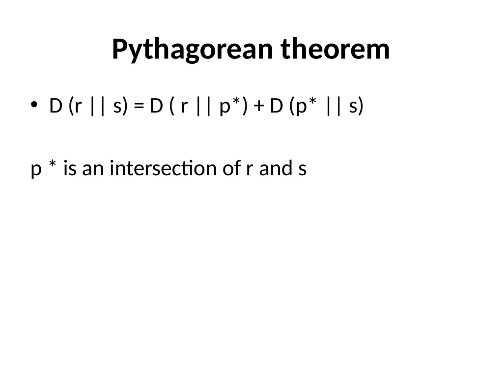
slide86. Pythagorean theorem D (r || s) = D ( r || p*) + D (p* || s)

p * is an intersection of r and s<br>
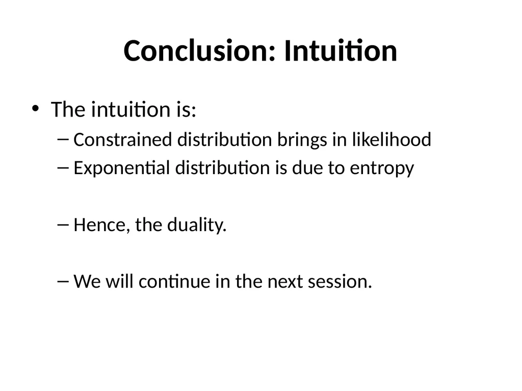
slide87. Conclusion: Intuition The intuition is:
Constrained distribution brings in likelihood
Exponential distribution is due to entropy

Hence, the duality.

We will continue in the next session.<br>
slide88. Maximum Likelihood-Maximum Entropy Duality: Session 7 Pushpak Bhattacharyya

Scribed by Aditya Joshi
Presented in NLP-AI talk on 20th September, 2015<br>
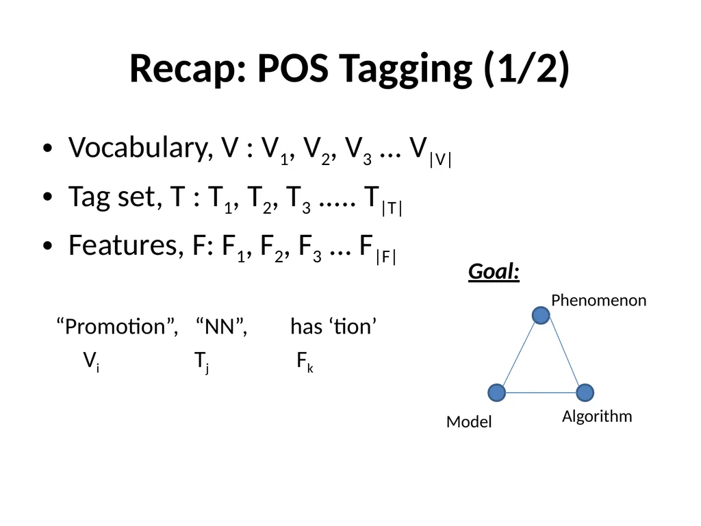
slide89. Recap: POS Tagging (1/2) Vocabulary, V : V1, V2, V3 ... V|V|
Tag set, T : T1, T2, T3 ..... T|T|
Features, F: F1, F2, F3 ... F|F| “Promotion”, “NN”, has ‘tion’ Vi Tj Fk Goal: Phenomenon Algorithm Model<br>
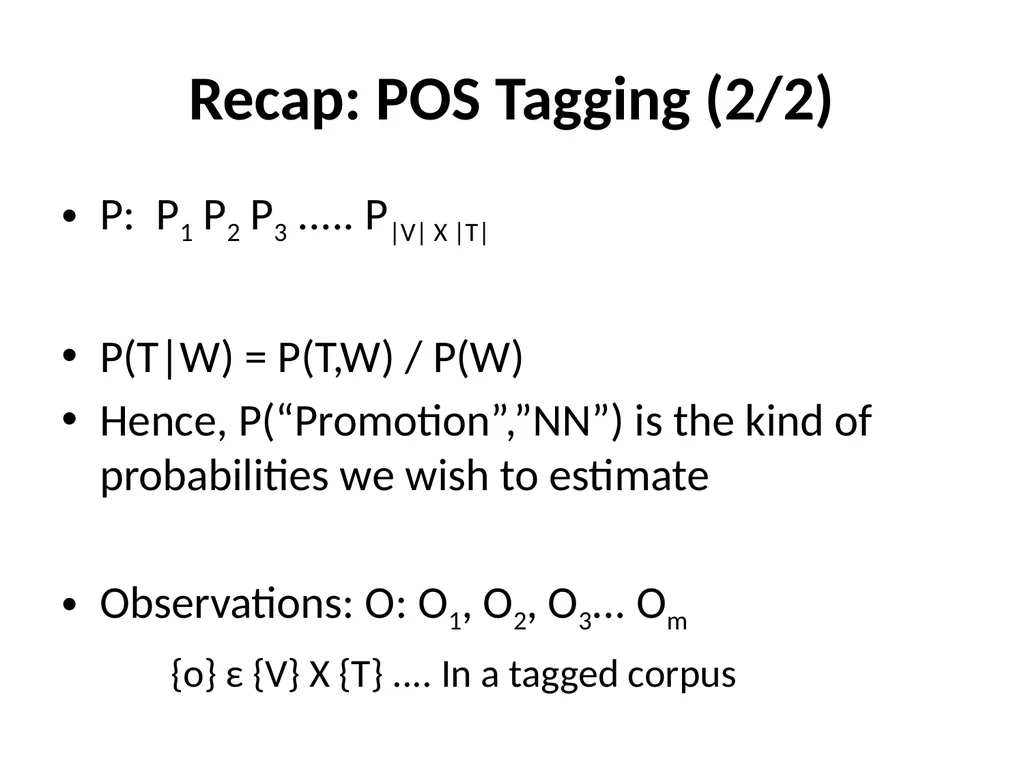
slide90. Recap: POS Tagging (2/2) P: P1 P2 P3 ..... P|V| X |T|

P(T|W) = P(T,W) / P(W)
Hence, P(“Promotion”,”NN”) is the kind of probabilities we wish to estimate

Observations: O: O1, O2, O3... Om {o} ε {V} X {T} .... In a tagged corpus<br>
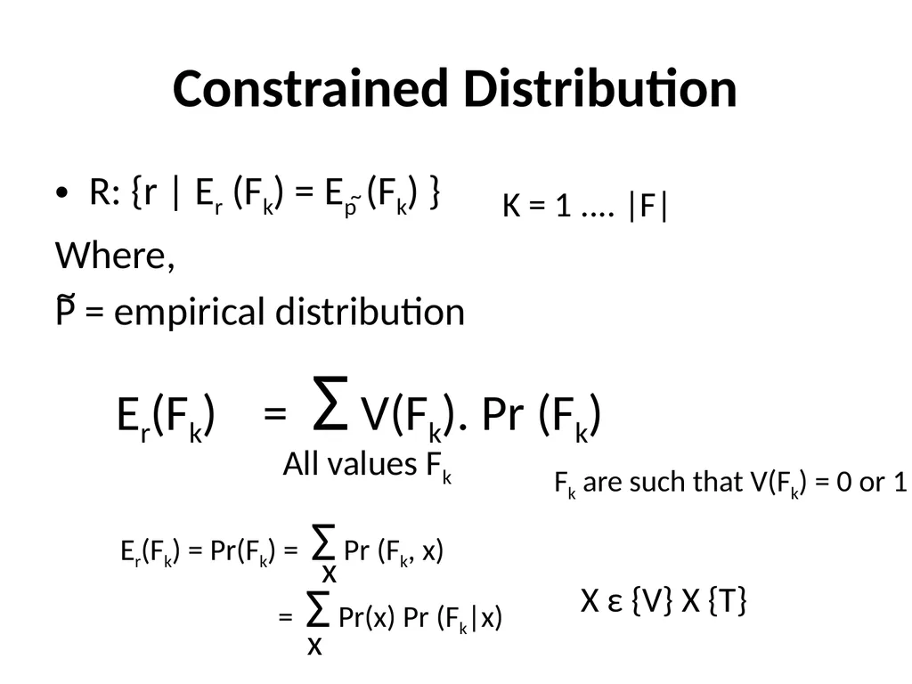
slide91. Constrained Distribution R: {r | Er (Fk) = Ep (Fk) }
Where,
P = empirical distribution ~ K = 1 .... |F| ~ Er(Fk) = Σ V(Fk). Pr (Fk) All values Fk Fk are such that V(Fk) = 0 or 1 Er(Fk) = Pr(Fk) = Σ Pr (Fk, x)
= Σ Pr(x) Pr (Fk|x) X ε {V} X {T} x x<br>
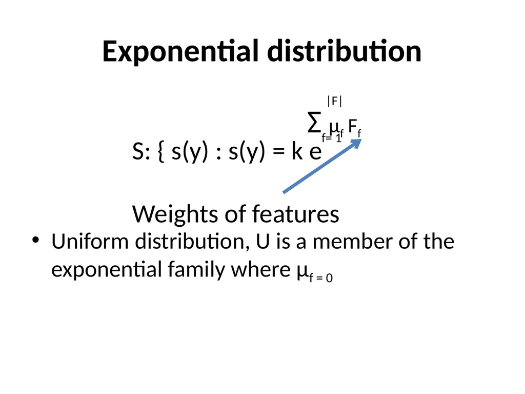
slide92. Exponential distribution Uniform distribution, U is a member of the exponential family where μf = 0 S: { s(y) : s(y) = k e

Weights of features Σ μf Ff f= 1 |F|<br>
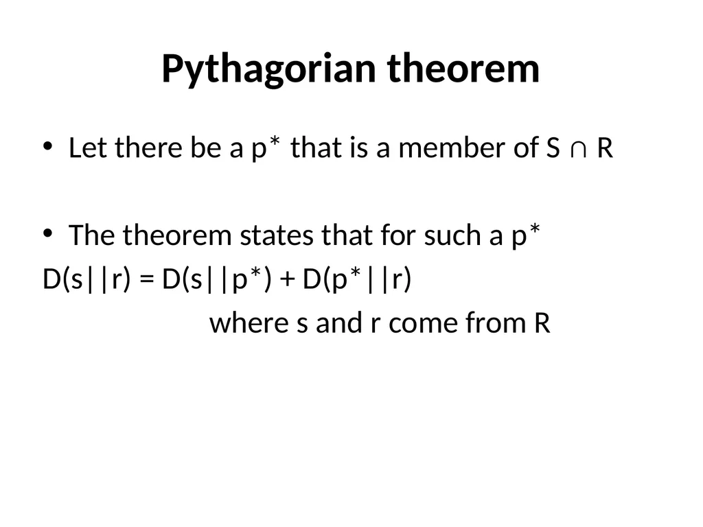
slide93. Pythagorian theorem Let there be a p* that is a member of S ∩ R

The theorem states that for such a p*
D(s||r) = D(s||p*) + D(p*||r)
where s and r come from R<br>
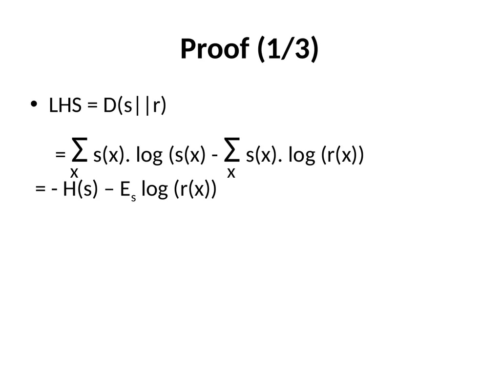
slide94. Proof (1/3) LHS = D(s||r)
= Σ s(x). log (s(x) - Σ s(x). log (r(x))
= - H(s) – Es log (r(x)) x x<br>
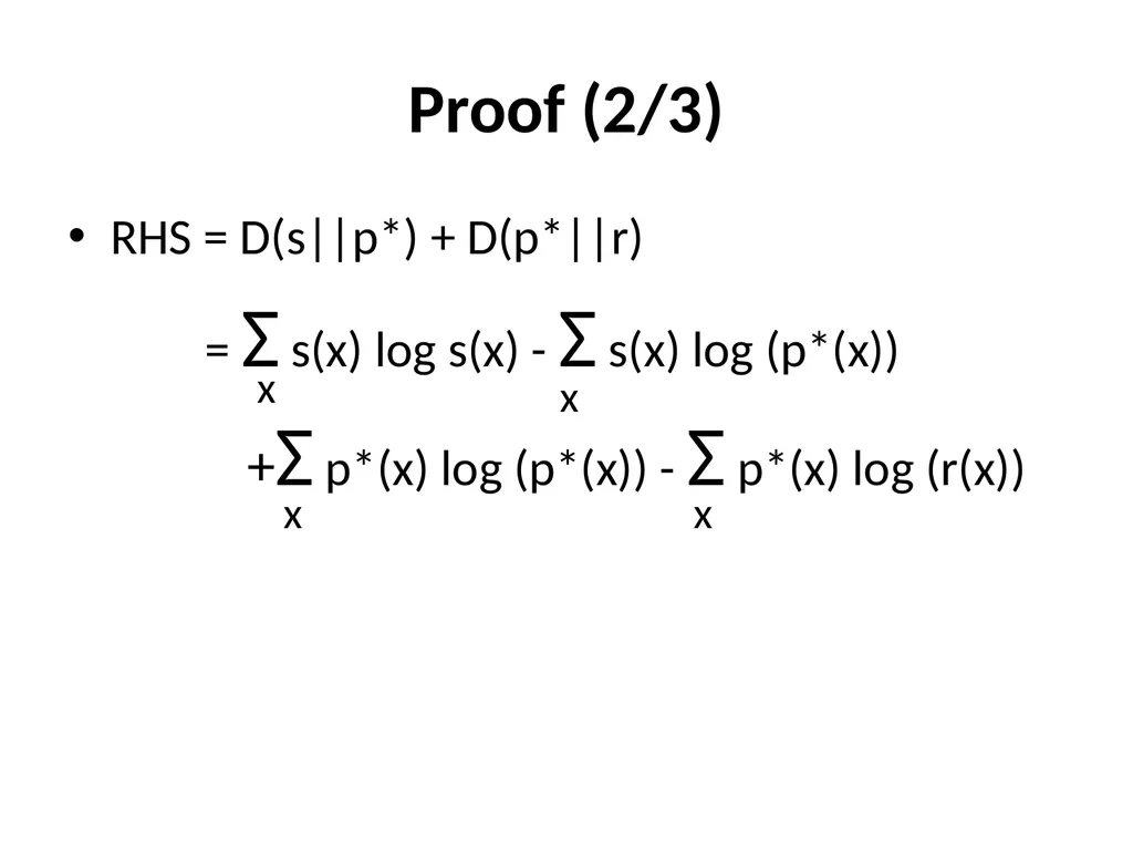
slide95. Proof (2/3) RHS = D(s||p*) + D(p*||r)
= Σ s(x) log s(x) - Σ s(x) log (p*(x))
+Σ p*(x) log (p*(x)) - Σ p*(x) log (r(x)) x x x x<br>
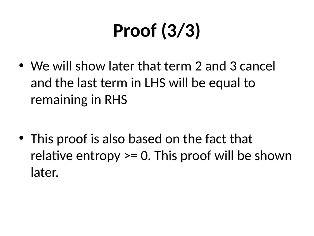
slide96. Proof (3/3) We will show later that term 2 and 3 cancel and the last term in LHS will be equal to remaining in RHS

This proof is also based on the fact that relative entropy >= 0. This proof will be shown later.<br>
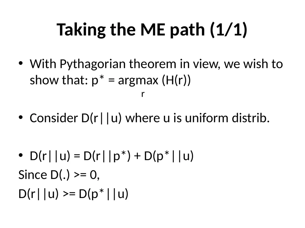
slide97. Taking the ME path (1/1) With Pythagorian theorem in view, we wish to show that: p* = argmax (H(r))

Consider D(r||u) where u is uniform distrib.

D(r||u) = D(r||p*) + D(p*||u)
Since D(.) >= 0,
D(r||u) >= D(p*||u) r<br>
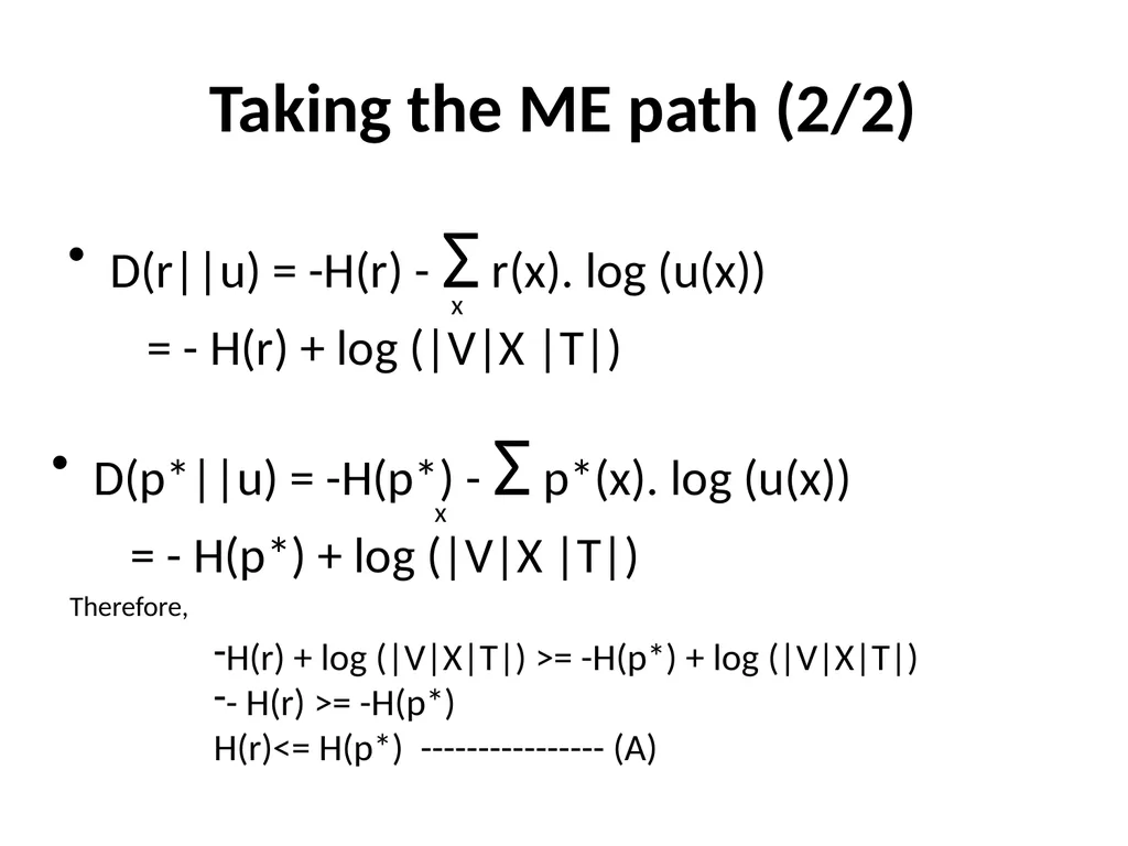
slide98. Taking the ME path (2/2) D(r||u) = -H(r) - Σ r(x). log (u(x))
= - H(r) + log (|V|X |T|) x D(p*||u) = -H(p*) - Σ p*(x). log (u(x))
= - H(p*) + log (|V|X |T|) x Therefore, H(r) + log (|V|X|T|) >= -H(p*) + log (|V|X|T|)
- H(r) >= -H(p*)
H(r)<= H(p*) ---------------- (A)<br>
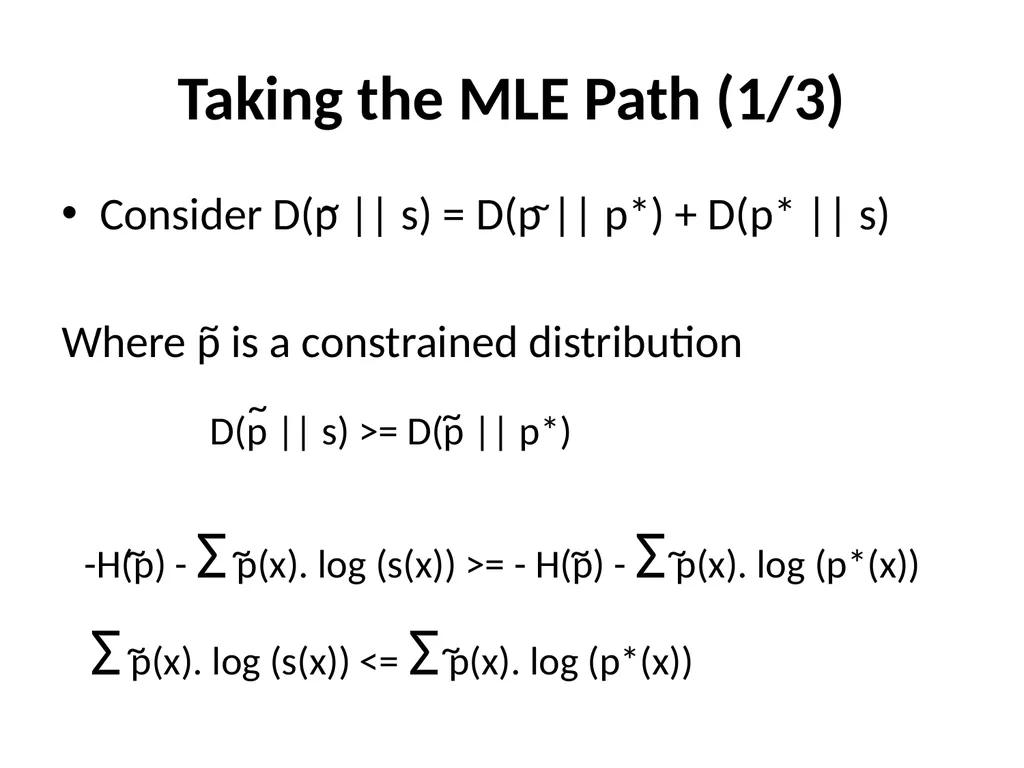
slide99. Taking the MLE Path (1/3) Consider D(p || s) = D(p || p*) + D(p* || s)

Where p is a constrained distribution ~ ~ ~ D(p || s) >= D(p || p*) ~ ~ -H(p) - Σ p(x). log (s(x)) >= - H(p) - Σ p(x). log (p*(x)) ~ ~ Σ p(x). log (s(x)) <= Σ p(x). log (p*(x)) ~ ~ ~ ~<br>
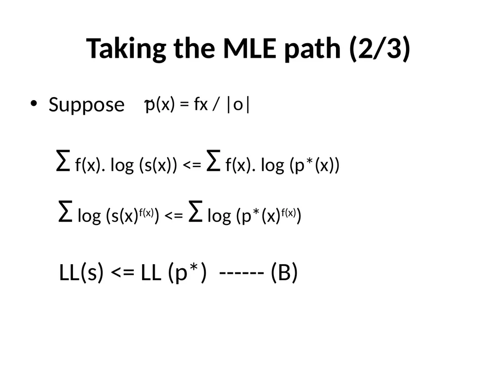
slide100. Taking the MLE path (2/3) Suppose p(x) = fx / |o| ~ Σ f(x). log (s(x)) <= Σ f(x). log (p*(x)) Σ log (s(x)f(x)) <= Σ log (p*(x)f(x)) LL(s) <= LL (p*) ------ (B)<br>
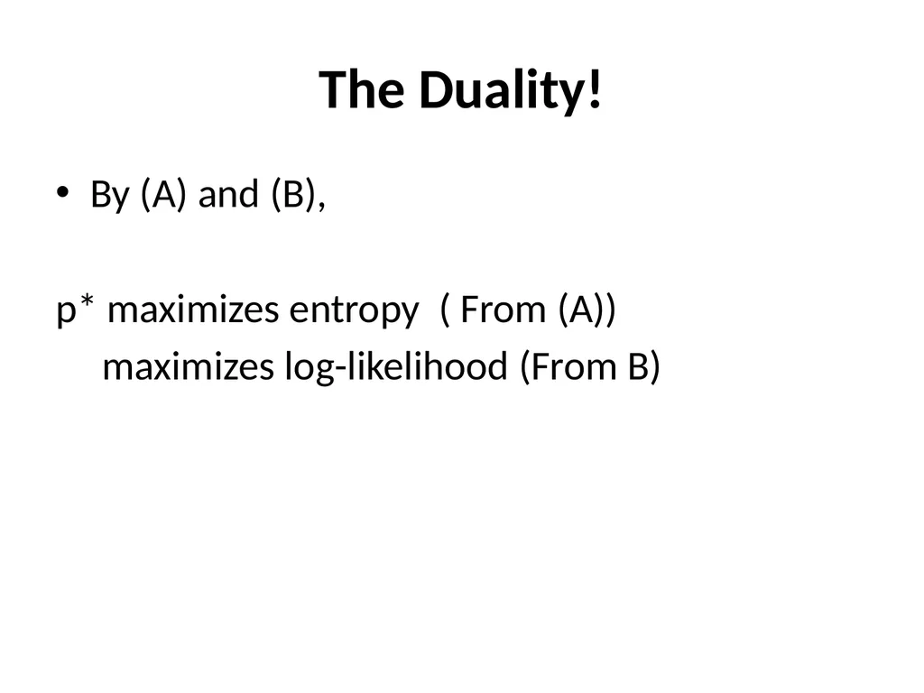
slide101. The Duality! By (A) and (B),

p* maximizes entropy ( From (A))
maximizes log-likelihood (From B)<br>
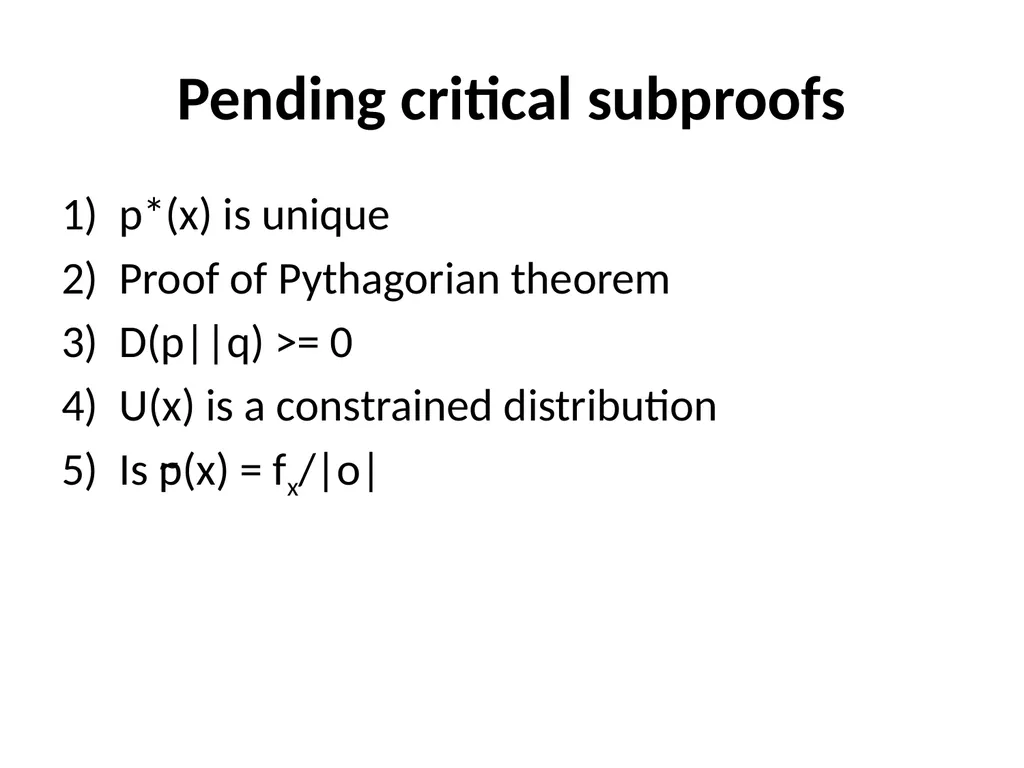
slide102. Pending critical subproofs p*(x) is unique
Proof of Pythagorian theorem
D(p||q) >= 0
U(x) is a constrained distribution
Is p(x) = fx/|o| ~<br>