
Modifications by A. Asef-Vaziri Chapter 4 Linear





Description: Modifications by A. Asef-Vaziri Chapter 4 Linear Programming Applications in Marketing, Finance, and Operations Marketing Applications Financial Applications Operations Management Applications Marketing Applications: Media Selection SMM
Related Topics
Download Presentation
"Modifications by A. Asef-Vaziri Chapter 4 Linear" is the property of its rightful owner. Permission is granted to download and print the materials on this website for personal, non-commercial use only, and to display it on your personal computer provided you do not modify the materials and that you retain all copyright notices contained in the materials. By downloading content from our website, you accept the terms of this agreement.
Presentation Transcript
slide1. Modifications by
A. Asef-Vaziri<br>
slide2. Chapter 4 Linear Programming Applications in Marketing, Finance, and Operations Marketing Applications
Financial Applications
Operations Management Applications<br>
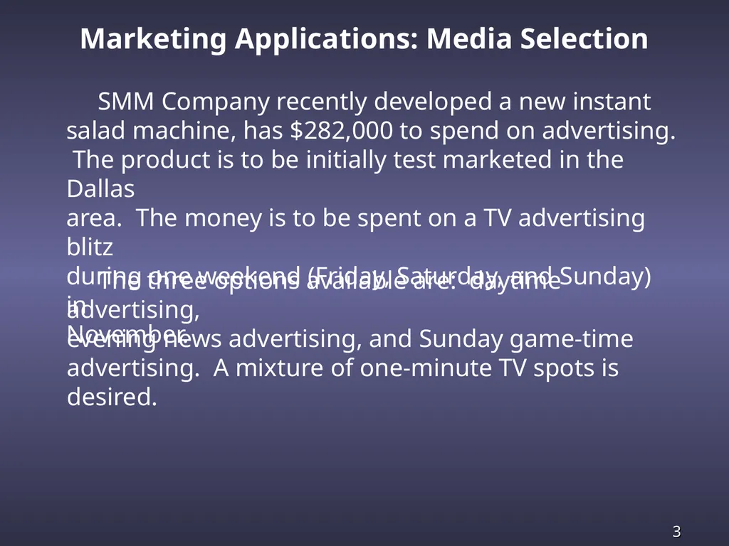
slide3. Marketing Applications: Media Selection SMM Company recently developed a new instant
salad machine, has $282,000 to spend on advertising. The product is to be initially test marketed in the Dallas
area. The money is to be spent on a TV advertising blitz
during one weekend (Friday, Saturday, and Sunday) in
November. The three options available are: daytime advertising,
evening news advertising, and Sunday game-time
advertising. A mixture of one-minute TV spots is desired.<br>
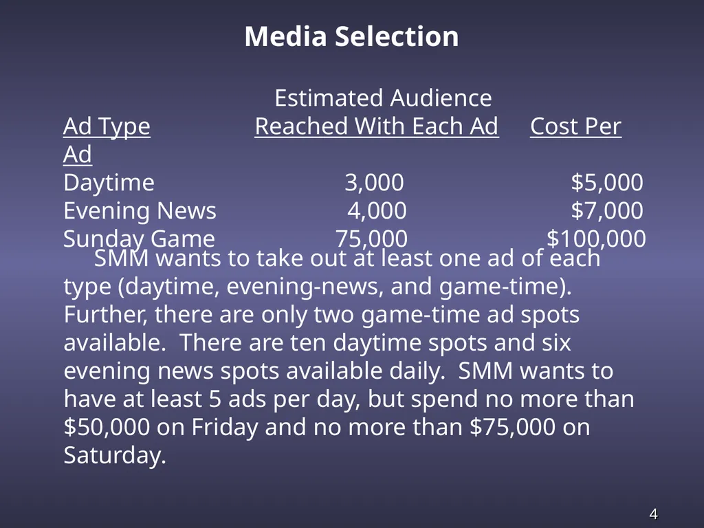
slide4. Media Selection Estimated Audience
Ad Type Reached With Each Ad Cost Per Ad
Daytime 3,000 $5,000
Evening News 4,000 $7,000
Sunday Game 75,000 $100,000 SMM wants to take out at least one ad of each type (daytime, evening-news, and game-time). Further, there are only two game-time ad spots available. There are ten daytime spots and six evening news spots available daily. SMM wants to have at least 5 ads per day, but spend no more than $50,000 on Friday and no more than $75,000 on Saturday.<br>
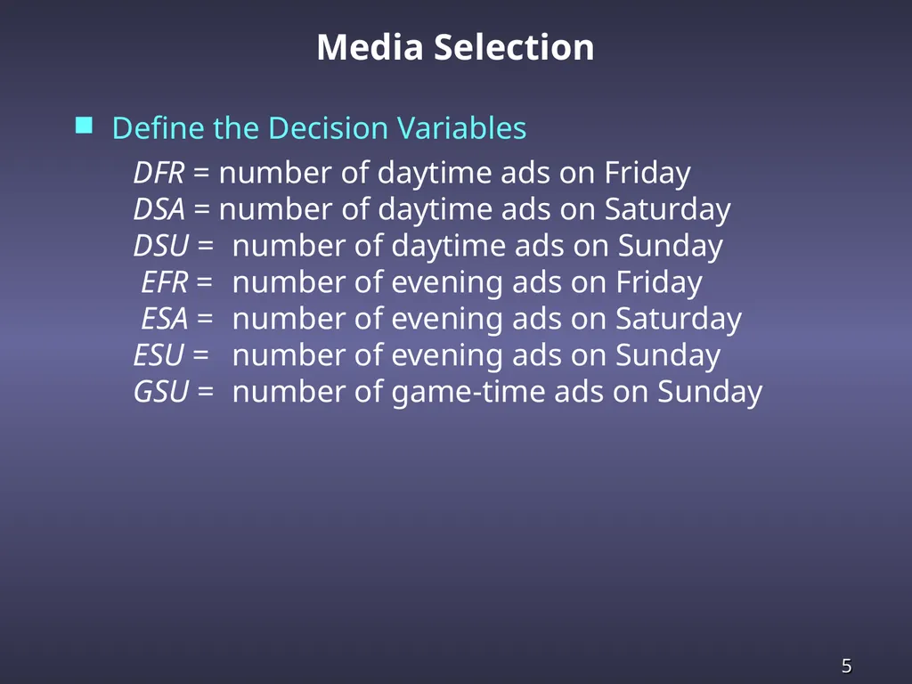
slide5. Media Selection DFR = number of daytime ads on Friday
DSA = number of daytime ads on Saturday
DSU = number of daytime ads on Sunday
EFR = number of evening ads on Friday
ESA = number of evening ads on Saturday
ESU = number of evening ads on Sunday
GSU = number of game-time ads on Sunday Define the Decision Variables<br>
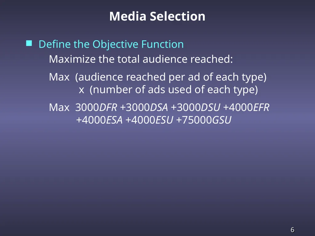
slide6. Media Selection Define the Objective Function Maximize the total audience reached:
Max (audience reached per ad of each type)
x (number of ads used of each type)
Max 3000DFR +3000DSA +3000DSU +4000EFR
+4000ESA +4000ESU +75000GSU<br>
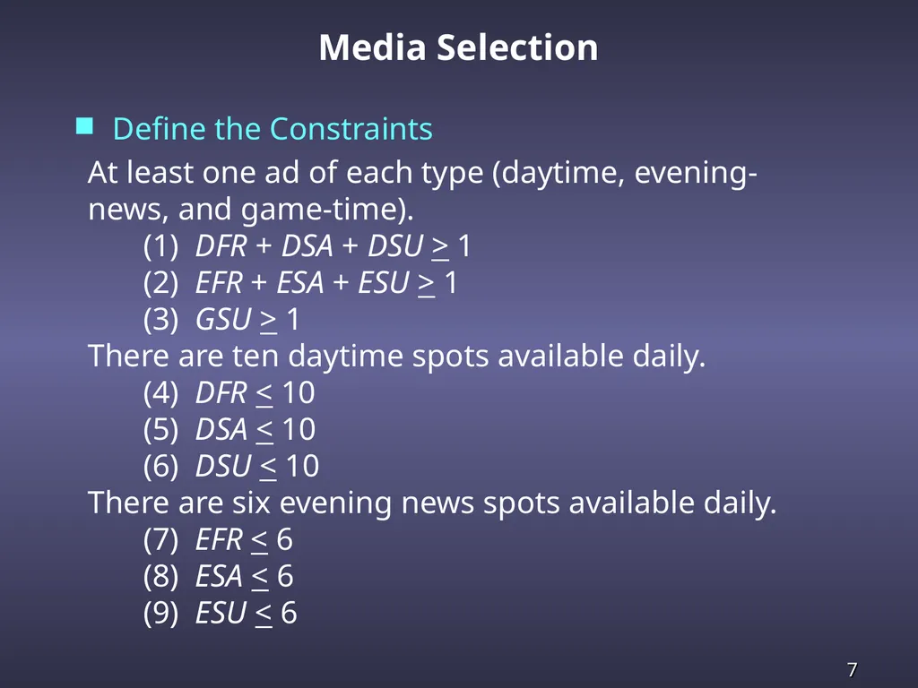
slide7. Media Selection Define the Constraints At least one ad of each type (daytime, evening-news, and game-time).
(1) DFR + DSA + DSU > 1
(2) EFR + ESA + ESU > 1
(3) GSU > 1
There are ten daytime spots available daily.
(4) DFR < 10
(5) DSA < 10
(6) DSU < 10
There are six evening news spots available daily.
(7) EFR < 6
(8) ESA < 6
(9) ESU < 6<br>
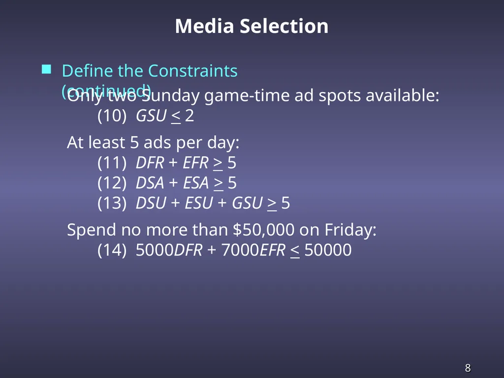
slide8. Media Selection Define the Constraints (continued) Only two Sunday game-time ad spots available:
(10) GSU < 2
At least 5 ads per day:
(11) DFR + EFR > 5
(12) DSA + ESA > 5
(13) DSU + ESU + GSU > 5
Spend no more than $50,000 on Friday:
(14) 5000DFR + 7000EFR < 50000<br>
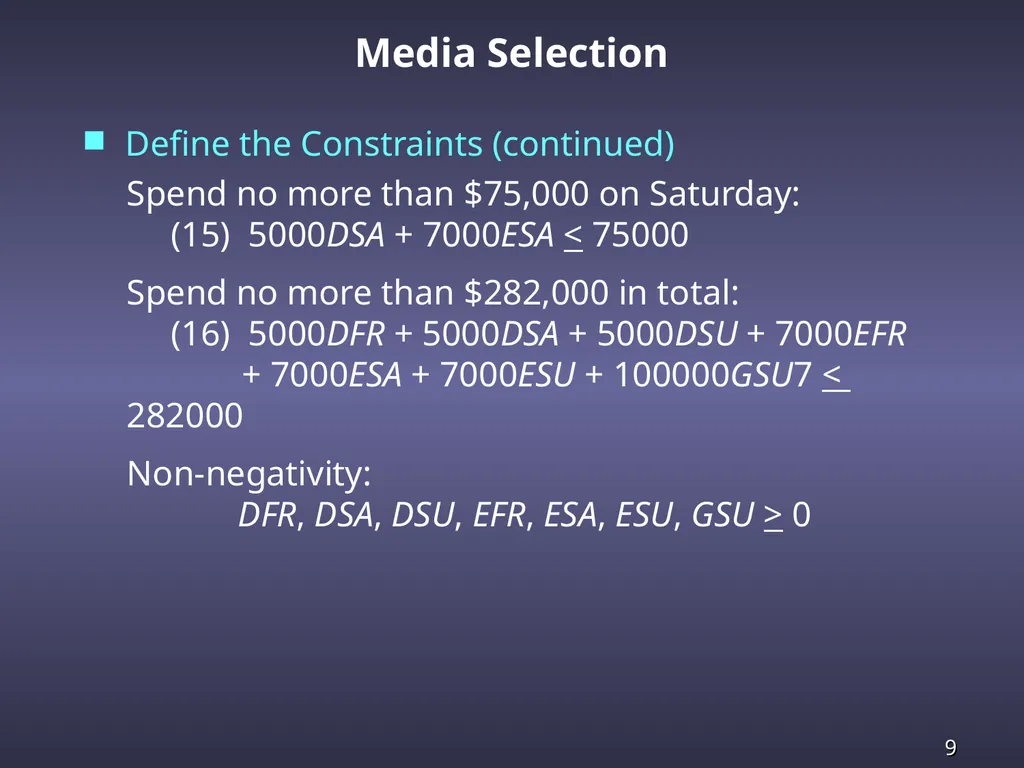
slide9. Media Selection Define the Constraints (continued) Spend no more than $75,000 on Saturday:
(15) 5000DSA + 7000ESA < 75000
Spend no more than $282,000 in total:
(16) 5000DFR + 5000DSA + 5000DSU + 7000EFR
+ 7000ESA + 7000ESU + 100000GSU7 < 282000
Non-negativity:
DFR, DSA, DSU, EFR, ESA, ESU, GSU > 0<br>
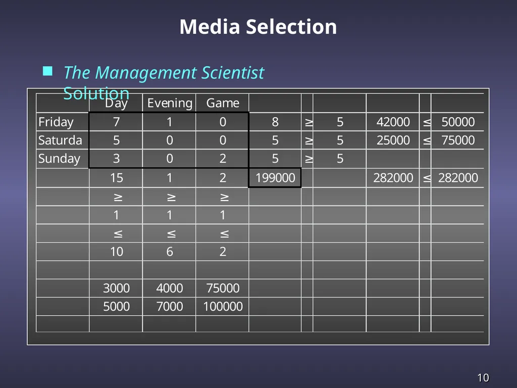
slide10. Media Selection The Management Scientist Solution<br>
slide11. A firm conducts marketing research to learn about consumer characteristics, attitudes, and preferences.
Marketing research services include designing the study, conducting surveys, analyzing data collected, and providing recommendations for the client.
In the research design phase, targets or quotas may be established for the number and types of respondents to be surveyed.
The marketing research firm’s objective is to conduct the survey so as to meet the client’s needs at a minimum cost. Marketing Applications<br>
slide12. Marketing Research: Marketing Research Market Survey, Inc. (MSI) specializes in evaluating consumer reaction to new products, services, and advertising campaigns. A client firm requested MSI’s assistance in ascertaining consumer reaction to a recently marketed household product.
During meetings with the client, MSI agreed to conduct door-to-door personal interviews to obtain responses from households with children and households without children. In addition, MSI agreed to conduct both day and evening interviews.<br>
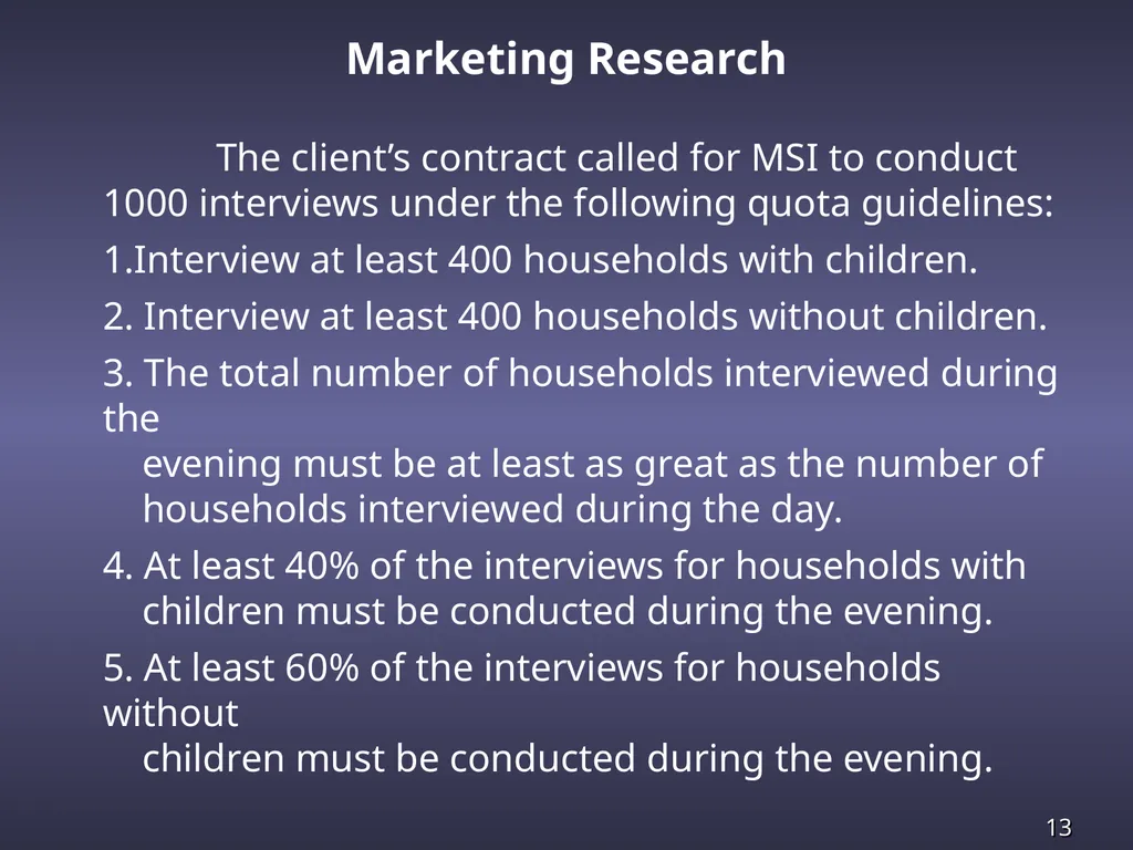
slide13. Marketing Research The client’s contract called for MSI to conduct 1000 interviews under the following quota guidelines:
Interview at least 400 households with children.
2. Interview at least 400 households without children.
3. The total number of households interviewed during the
evening must be at least as great as the number of
households interviewed during the day.
4. At least 40% of the interviews for households with
children must be conducted during the evening.
5. At least 60% of the interviews for households without
children must be conducted during the evening.<br>
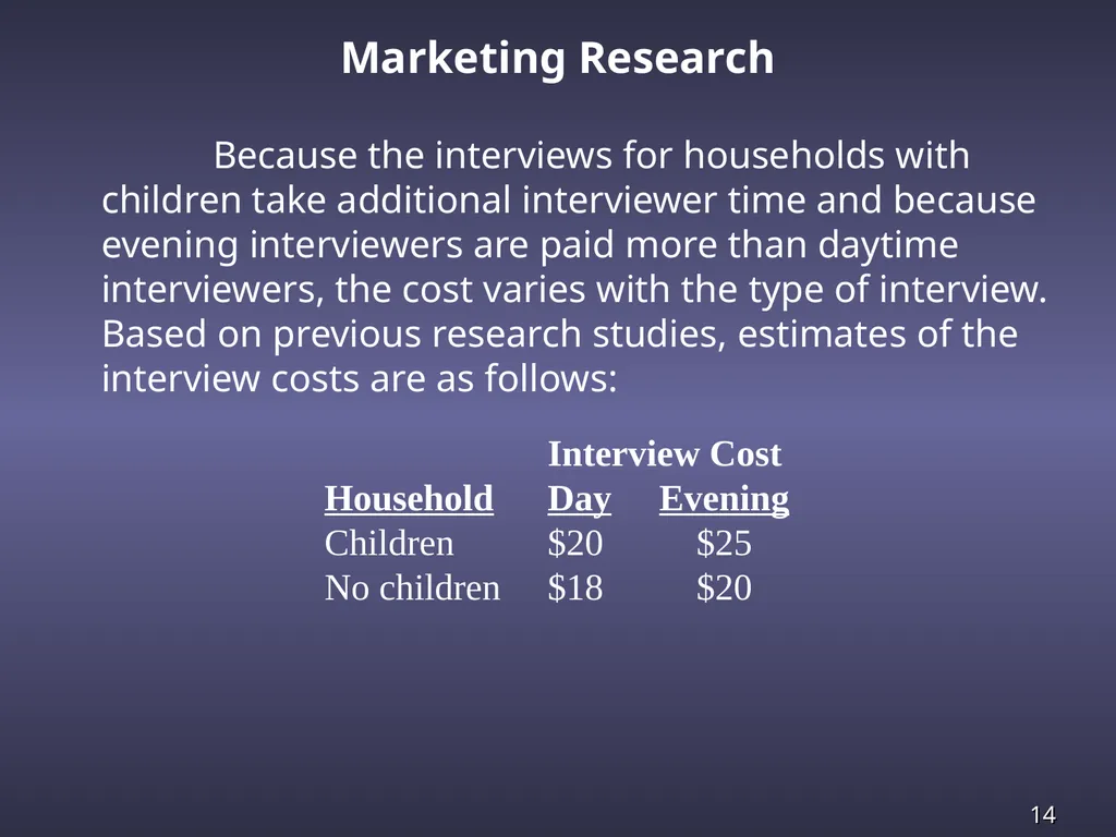
slide14. Marketing Research Because the interviews for households with children take additional interviewer time and because evening interviewers are paid more than daytime interviewers, the cost varies with the type of interview. Based on previous research studies, estimates of the interview costs are as follows:
Interview Cost
Household Day Evening
Children $20 $25
No children $18 $20<br>
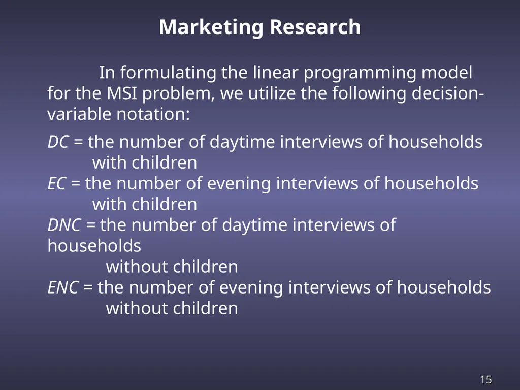
slide15. Marketing Research In formulating the linear programming model for the MSI problem, we utilize the following decision-variable notation:
DC = the number of daytime interviews of households
with children
EC = the number of evening interviews of households
with children
DNC = the number of daytime interviews of households
without children
ENC = the number of evening interviews of households
without children<br>
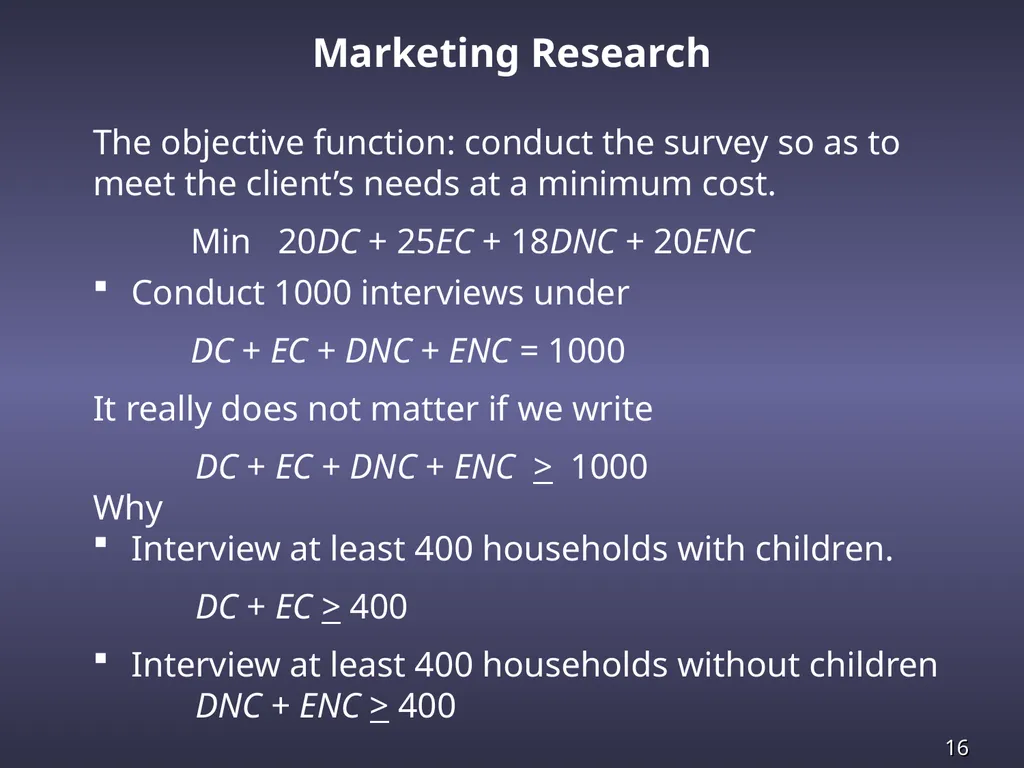
slide16. Marketing Research The objective function: conduct the survey so as to meet the client’s needs at a minimum cost.
Min 20DC + 25EC + 18DNC + 20ENC
Conduct 1000 interviews under
DC + EC + DNC + ENC = 1000
It really does not matter if we write
DC + EC + DNC + ENC > 1000
Why
Interview at least 400 households with children.
DC + EC > 400
Interview at least 400 households without children
DNC + ENC > 400<br>
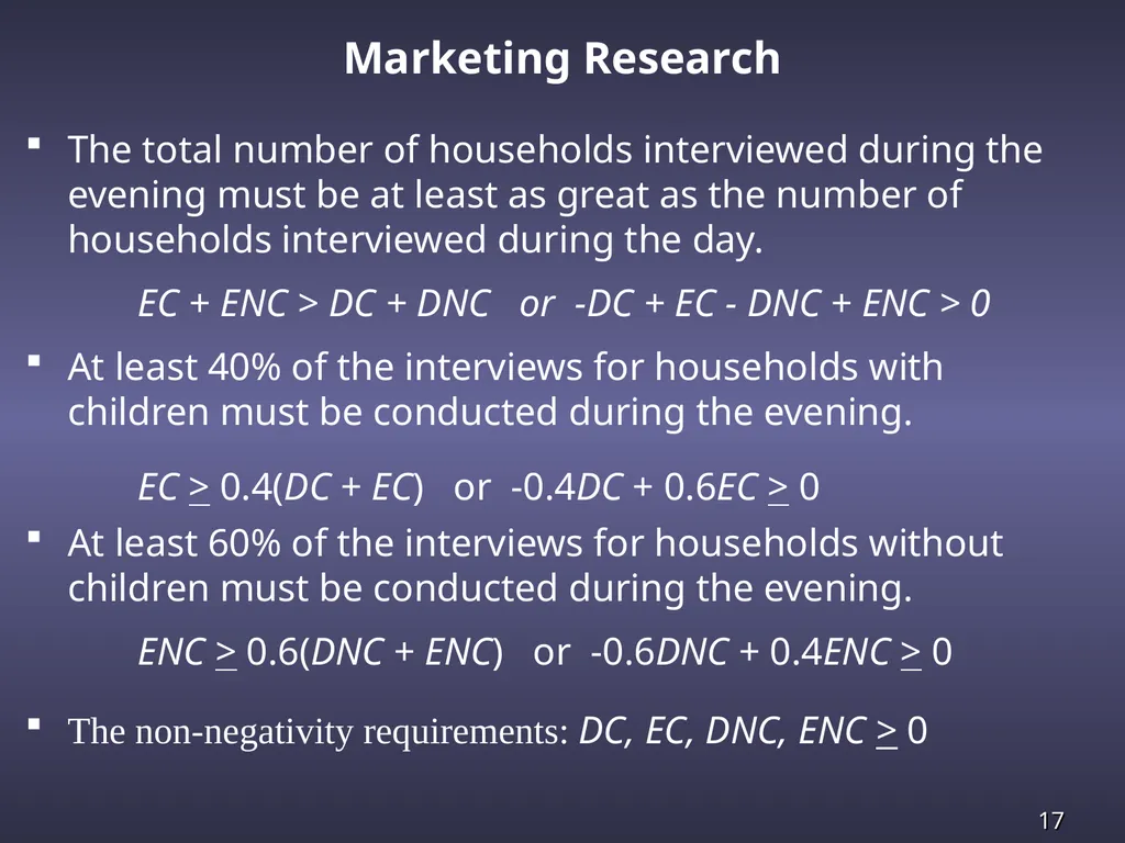
slide17. Marketing Research The total number of households interviewed during the evening must be at least as great as the number of households interviewed during the day.
EC + ENC > DC + DNC or -DC + EC - DNC + ENC > 0
At least 40% of the interviews for households with children must be conducted during the evening.
EC > 0.4(DC + EC) or -0.4DC + 0.6EC > 0
At least 60% of the interviews for households without children must be conducted during the evening.
ENC > 0.6(DNC + ENC) or -0.6DNC + 0.4ENC > 0
The non-negativity requirements: DC, EC, DNC, ENC > 0<br>
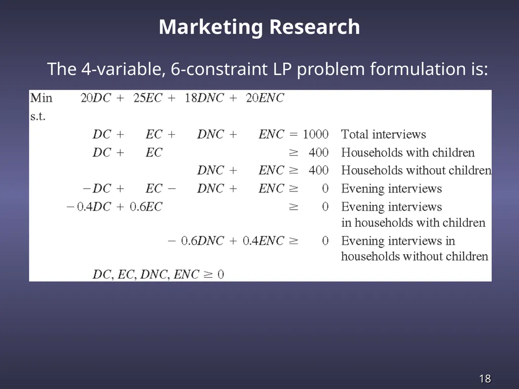
slide18. Marketing Research The 4-variable, 6-constraint LP problem formulation is:<br>
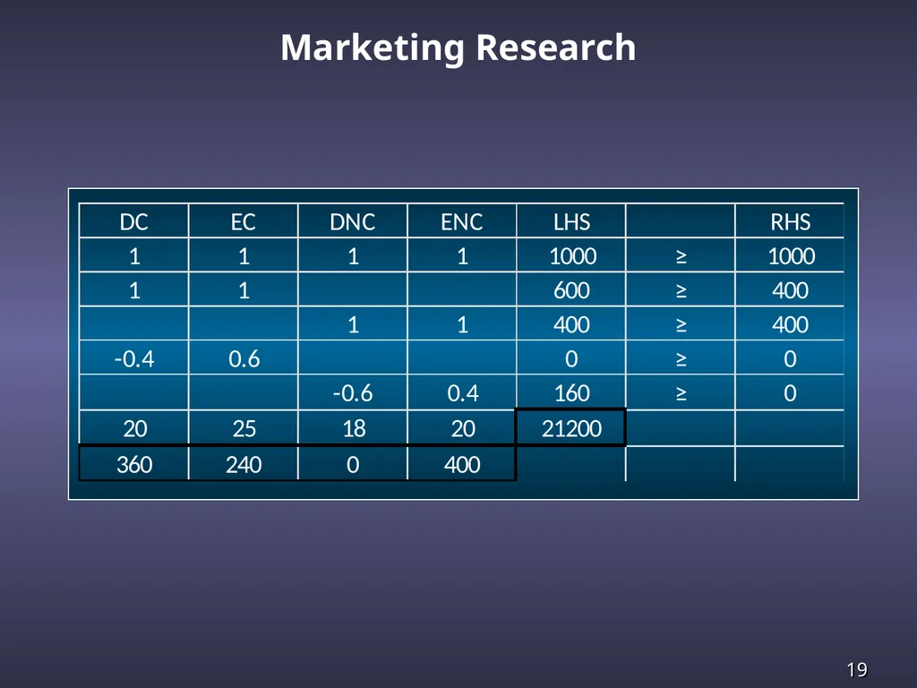
slide19. Marketing Research<br>
slide20. Financial Applications: Portfolio Selection Winslow Savings has $20 million available for
investment. It wishes to invest over the next four
months in such a way that it will maximize the total
interest earned over the four month period as well as
have at least $10 million available at the start of the
fifth month for a high rise building venture in which it
will be participating.<br>
slide21. Portfolio Selection For the time being, Winslow wishes to invest
only in 2-month government bonds (earning 2% over
the 2-month period) and 3-month construction loans
(earning 6% over the 3-month period). Each of these
is available each month for investment. Funds not
invested in these two investments are liquid and earn
3/4 of 1% per month when invested locally.<br>
slide22. Portfolio Selection Formulate a linear program that will help
Winslow Savings determine how to invest over the
next four months if at no time does it wish to have
more than $8 million in either government bonds or
construction loans.<br>
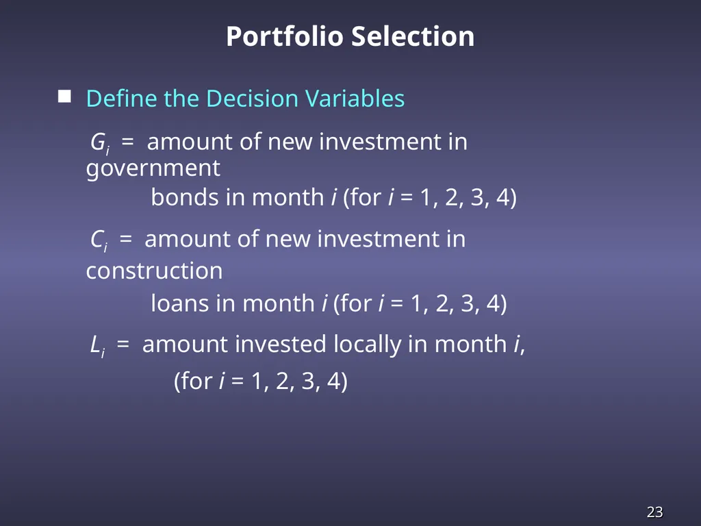
slide23. Portfolio Selection Define the Decision Variables
Gi = amount of new investment in government
bonds in month i (for i = 1, 2, 3, 4)
Ci = amount of new investment in construction
loans in month i (for i = 1, 2, 3, 4)
Li = amount invested locally in month i,
(for i = 1, 2, 3, 4)<br>
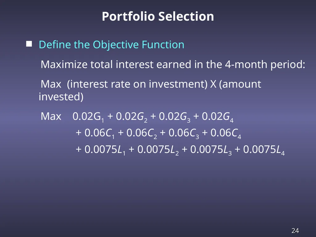
slide24. Portfolio Selection Define the Objective Function
Maximize total interest earned in the 4-month period:
Max (interest rate on investment) X (amount invested)
Max 0.02G1 + 0.02G2 + 0.02G3 + 0.02G4
+ 0.06C1 + 0.06C2 + 0.06C3 + 0.06C4
+ 0.0075L1 + 0.0075L2 + 0.0075L3 + 0.0075L4<br>
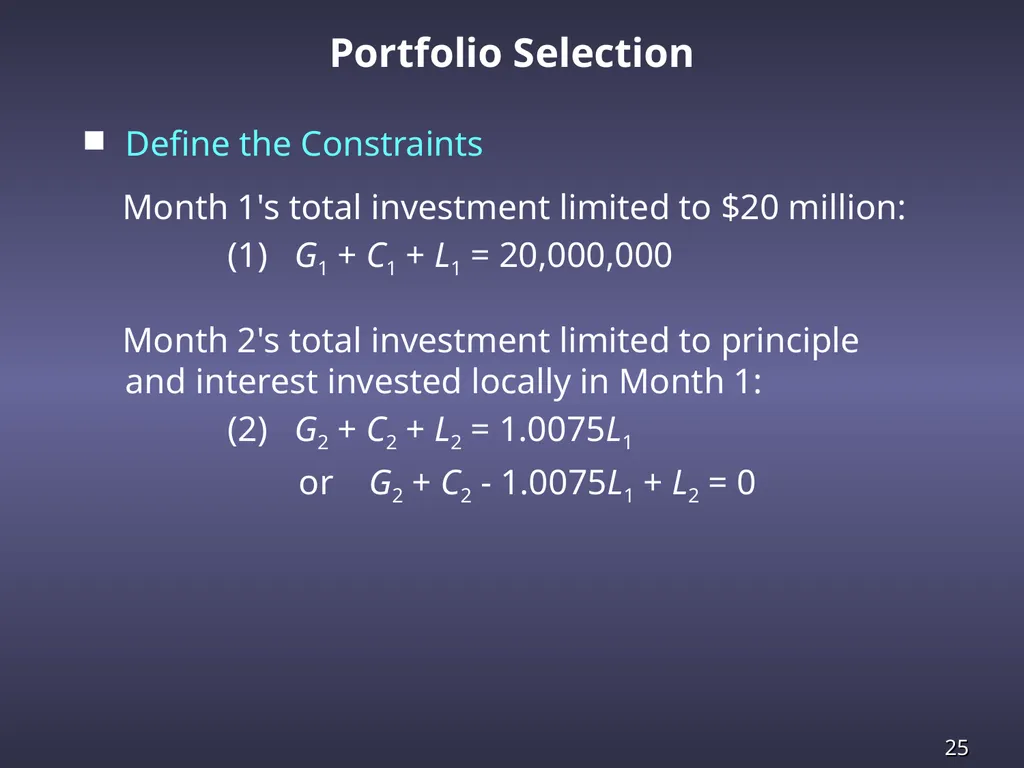
slide25. Portfolio Selection Define the Constraints
Month 1's total investment limited to $20 million:
(1) G1 + C1 + L1 = 20,000,000
Month 2's total investment limited to principle and interest invested locally in Month 1:
(2) G2 + C2 + L2 = 1.0075L1
or G2 + C2 - 1.0075L1 + L2 = 0<br>
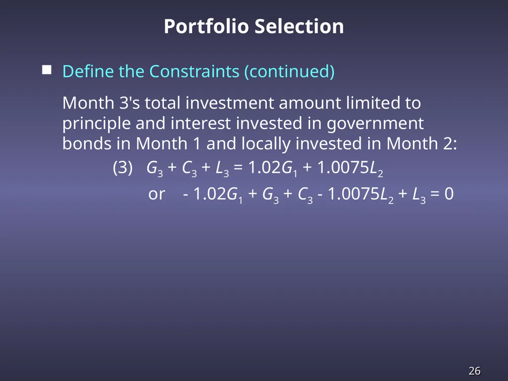
slide26. Portfolio Selection Define the Constraints (continued)
Month 3's total investment amount limited to principle and interest invested in government bonds in Month 1 and locally invested in Month 2:
(3) G3 + C3 + L3 = 1.02G1 + 1.0075L2
or - 1.02G1 + G3 + C3 - 1.0075L2 + L3 = 0<br>
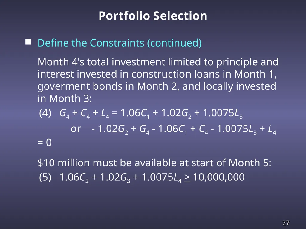
slide27. Portfolio Selection Define the Constraints (continued)
Month 4's total investment limited to principle and interest invested in construction loans in Month 1, goverment bonds in Month 2, and locally invested in Month 3:
(4) G4 + C4 + L4 = 1.06C1 + 1.02G2 + 1.0075L3
or - 1.02G2 + G4 - 1.06C1 + C4 - 1.0075L3 + L4 = 0
$10 million must be available at start of Month 5:
(5) 1.06C2 + 1.02G3 + 1.0075L4 > 10,000,000<br>
slide28. Portfolio Selection Define the Constraints (continued)
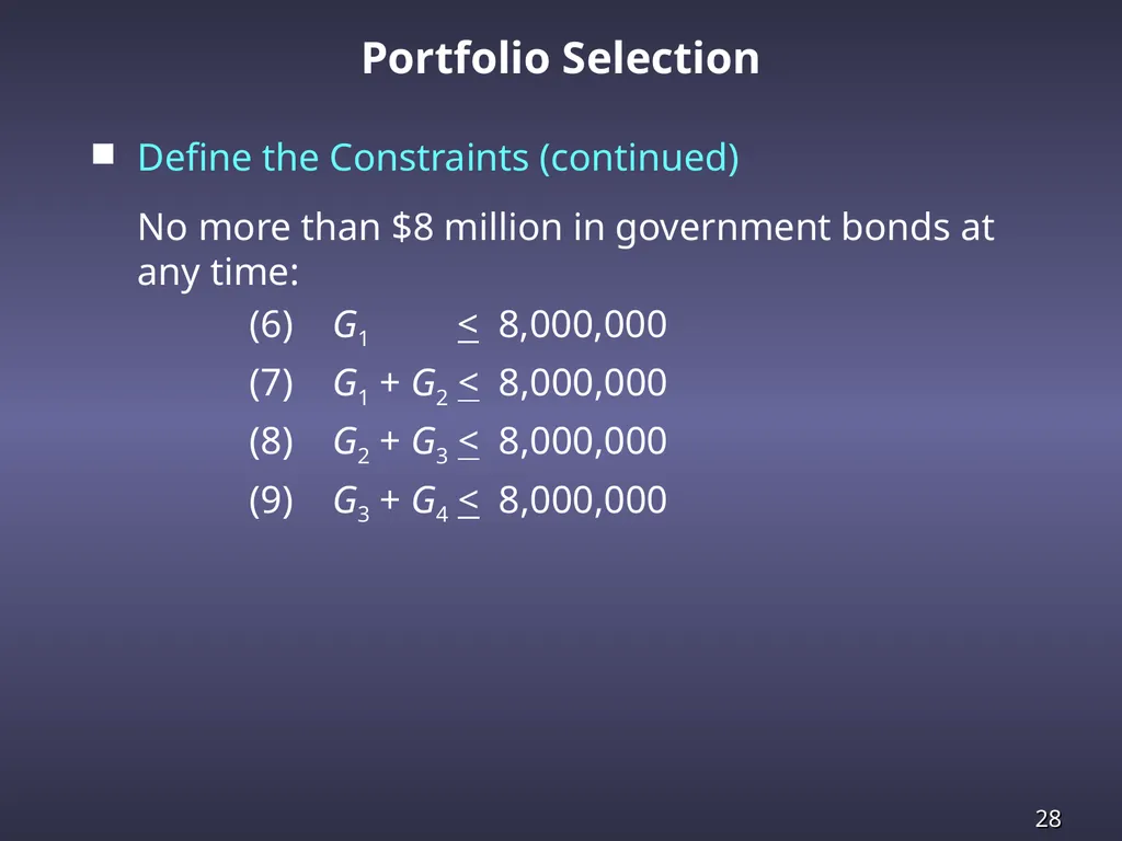
No more than $8 million in government bonds at any time:
(6) G1 < 8,000,000
(7) G1 + G2 < 8,000,000
(8) G2 + G3 < 8,000,000
(9) G3 + G4 < 8,000,000<br>
slide29. Portfolio Selection Define the Constraints (continued)
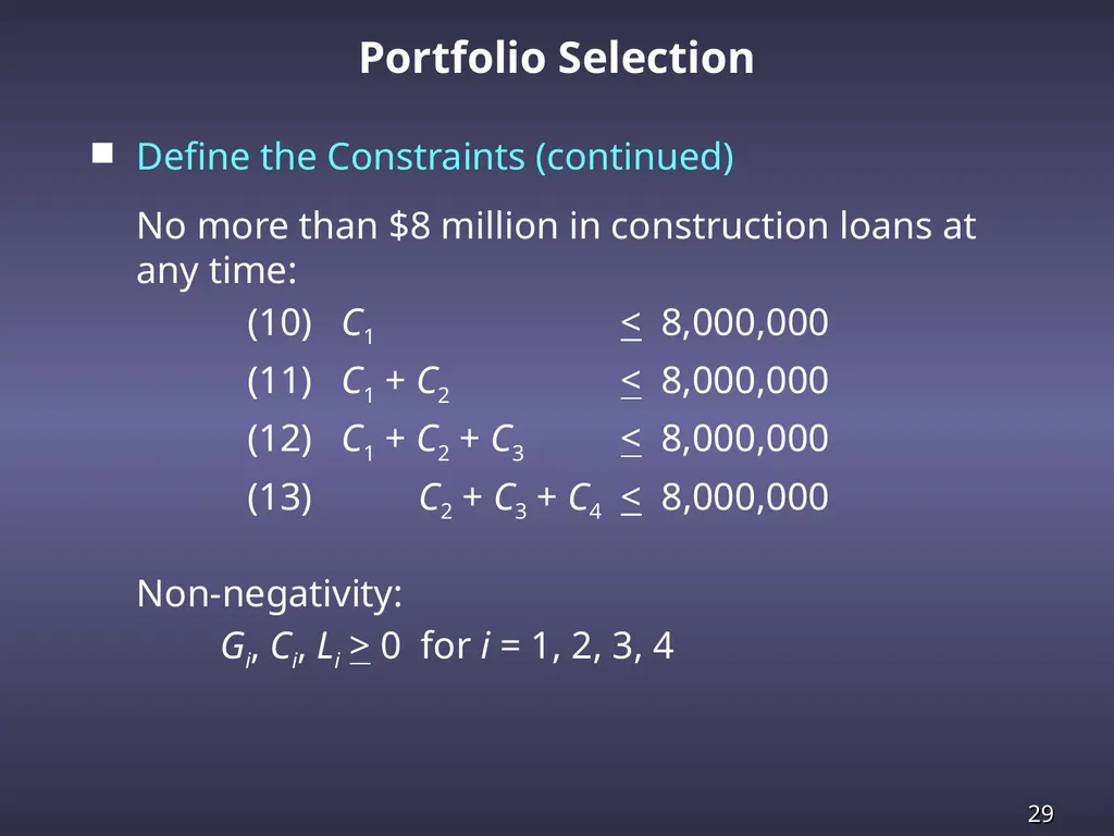
No more than $8 million in construction loans at any time:
(10) C1 < 8,000,000
(11) C1 + C2 < 8,000,000
(12) C1 + C2 + C3 < 8,000,000
(13) C2 + C3 + C4 < 8,000,000
Non-negativity:
Gi, Ci, Li > 0 for i = 1, 2, 3, 4<br>
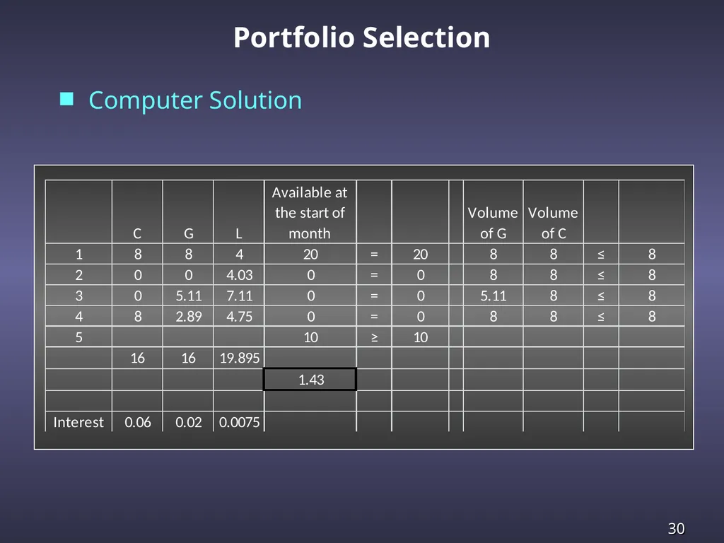
slide30. Portfolio Selection Computer Solution<br>
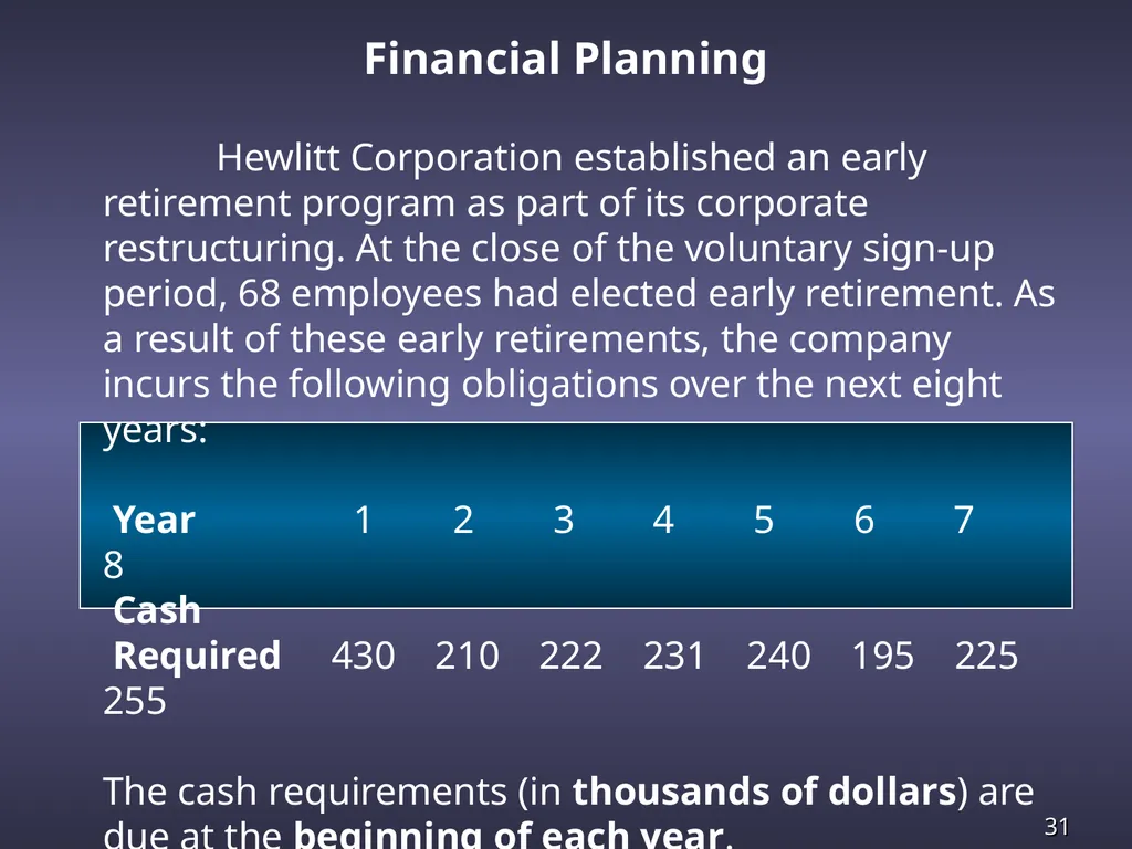
slide31. Financial Planning Hewlitt Corporation established an early retirement program as part of its corporate restructuring. At the close of the voluntary sign-up period, 68 employees had elected early retirement. As a result of these early retirements, the company incurs the following obligations over the next eight years:
Year 1 2 3 4 5 6 7 8
Cash
Required 430 210 222 231 240 195 225 255
The cash requirements (in thousands of dollars) are due at the beginning of each year.<br>
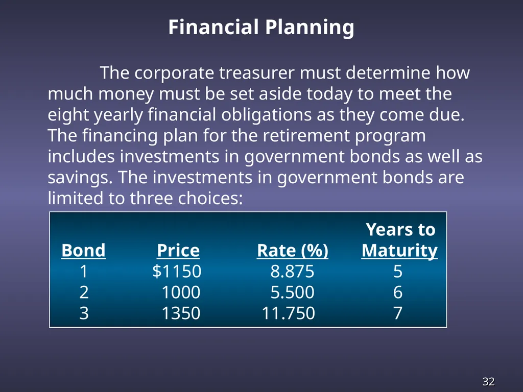
slide32. Financial Planning The corporate treasurer must determine how much money must be set aside today to meet the eight yearly financial obligations as they come due. The financing plan for the retirement program includes investments in government bonds as well as savings. The investments in government bonds are limited to three choices:
Years to
Bond Price Rate (%) Maturity
1 $1150 8.875 5
2 1000 5.500 6
3 1350 11.750 7<br>
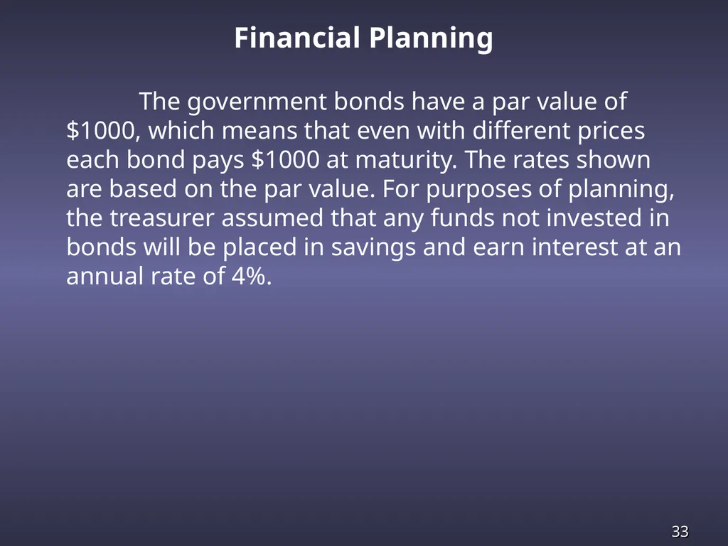
slide33. Financial Planning The government bonds have a par value of $1000, which means that even with different prices each bond pays $1000 at maturity. The rates shown are based on the par value. For purposes of planning, the treasurer assumed that any funds not invested in bonds will be placed in savings and earn interest at an annual rate of 4%.<br>
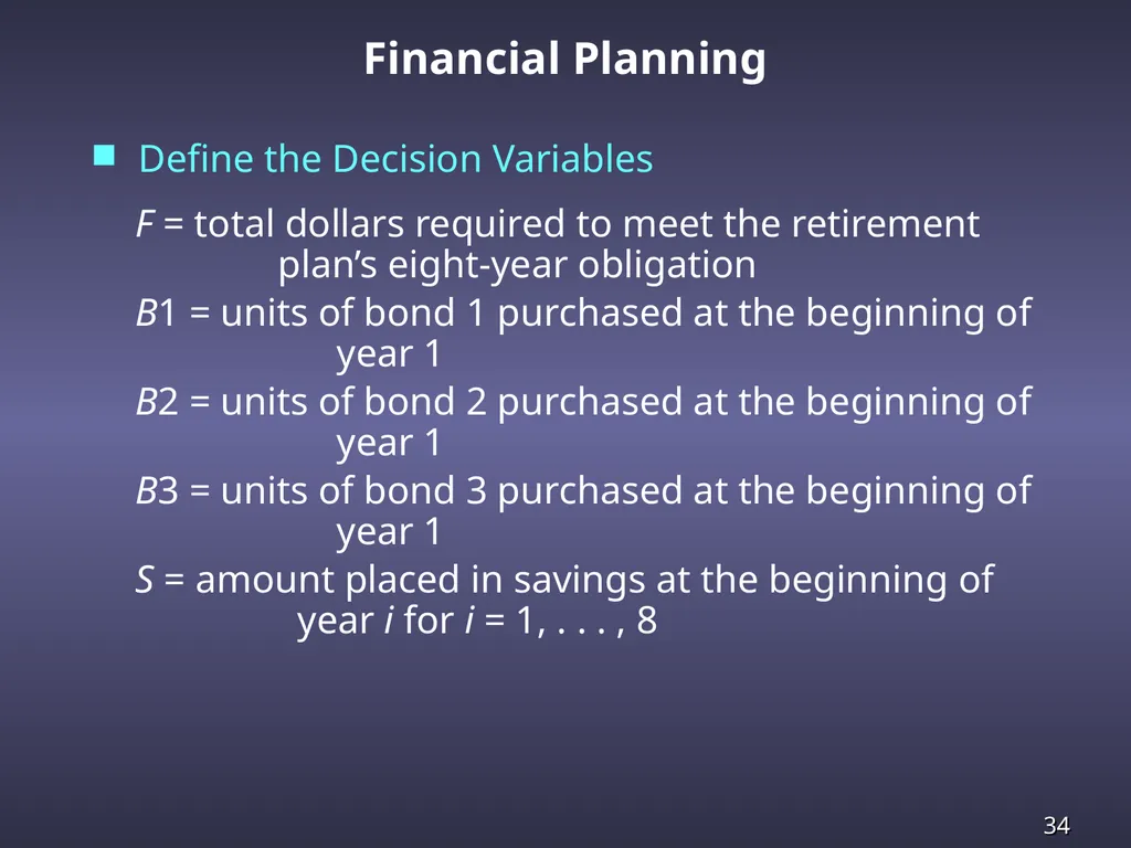
slide34. Financial Planning Define the Decision Variables
F = total dollars required to meet the retirement plan’s eight-year obligation
B1 = units of bond 1 purchased at the beginning of year 1
B2 = units of bond 2 purchased at the beginning of year 1
B3 = units of bond 3 purchased at the beginning of year 1
S = amount placed in savings at the beginning of year i for i = 1, . . . , 8<br>
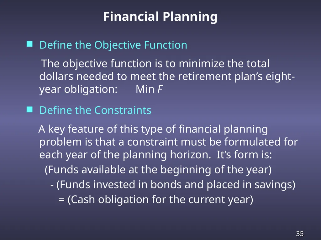
slide35. Financial Planning Define the Objective Function
The objective function is to minimize the total dollars needed to meet the retirement plan’s eight-year obligation: Min F
Define the Constraints
A key feature of this type of financial planning problem is that a constraint must be formulated for each year of the planning horizon. It’s form is:
(Funds available at the beginning of the year)
- (Funds invested in bonds and placed in savings)
= (Cash obligation for the current year)<br>
slide36. Financial Planning Define the Constraints
A constraint must be formulated for each year of the planning horizon in the following form:
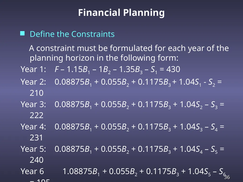
Year 1: F – 1.15B1 – 1B2 – 1.35B3 – S1 = 430
Year 2: 0.08875B1 + 0.055B2 + 0.1175B3 + 1.04S1 - S2 = 210
Year 3: 0.08875B1 + 0.055B2 + 0.1175B3 + 1.04S2 – S3 = 222
Year 4: 0.08875B1 + 0.055B2 + 0.1175B3 + 1.04S3 – S4 = 231
Year 5: 0.08875B1 + 0.055B2 + 0.1175B3 + 1.04S4 – S5 = 240
Year 6 1.08875B1 + 0.055B2 + 0.1175B3 + 1.04S5 – S6 = 195
Year 7: 1.055B2 + 0.1175B3 + 1.04S6 – S7 = 225
Year 8: 1.1175B3 + 1.04S7 – S8 = 255<br>
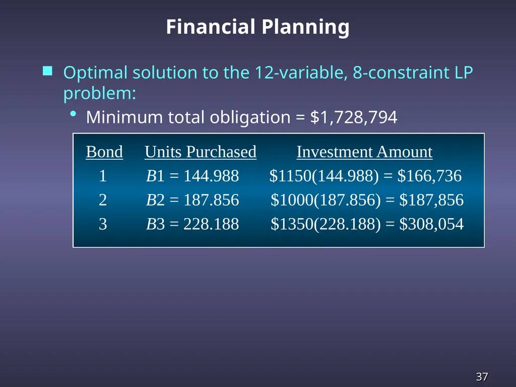
slide37. Financial Planning Optimal solution to the 12-variable, 8-constraint LP problem:
Minimum total obligation = $1,728,794
Bond Units Purchased Investment Amount
1 B1 = 144.988 $1150(144.988) = $166,736
2 B2 = 187.856 $1000(187.856) = $187,856
3 B3 = 228.188 $1350(228.188) = $308,054<br>
slide38. Operations Management Applications LP can be used in operations management to aid in decision-making about product mix, production scheduling, staffing, inventory control, capacity planning, and other issues.
An important application of LP is multi-period planning such as production scheduling.
Usually the objective is to establish an efficient, low-cost production schedule for one or more products over several time periods.
Typical constraints include limitations on production capacity, labor capacity, storage space, and more.<br>
slide39. Chip Hoose is the owner of Hoose Custom Wheels. Chip has just received orders for 1,000 standard wheels
and 1,250 deluxe wheels next month and for 800 standard and 1,500 deluxe the following month. All
orders must be filled. Operations Management Applications
Production Scheduling The cost of making standard wheels is $10 and deluxe
wheels is $16. Overtime rates are 50% higher. There
are 1,000 hours of regular time and 500 hours of overtime available each month. It takes 0.5 hour to make a standard wheel and 0.6 hour to make a deluxe wheel.
The cost of storing a wheel from one month to the next is $2.<br>
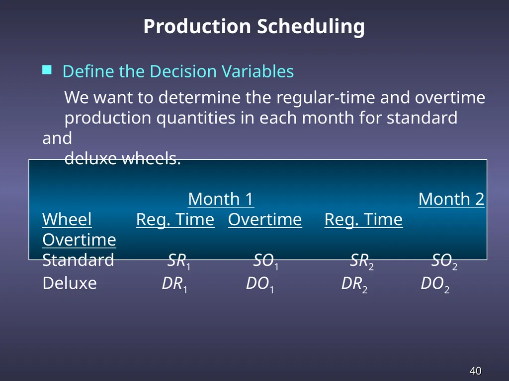
slide40. Production Scheduling We want to determine the regular-time and overtime
production quantities in each month for standard and
deluxe wheels.
Month 1 Month 2
Wheel Reg. Time Overtime Reg. Time Overtime
Standard SR1 SO1 SR2 SO2
Deluxe DR1 DO1 DR2 DO2 Define the Decision Variables<br>
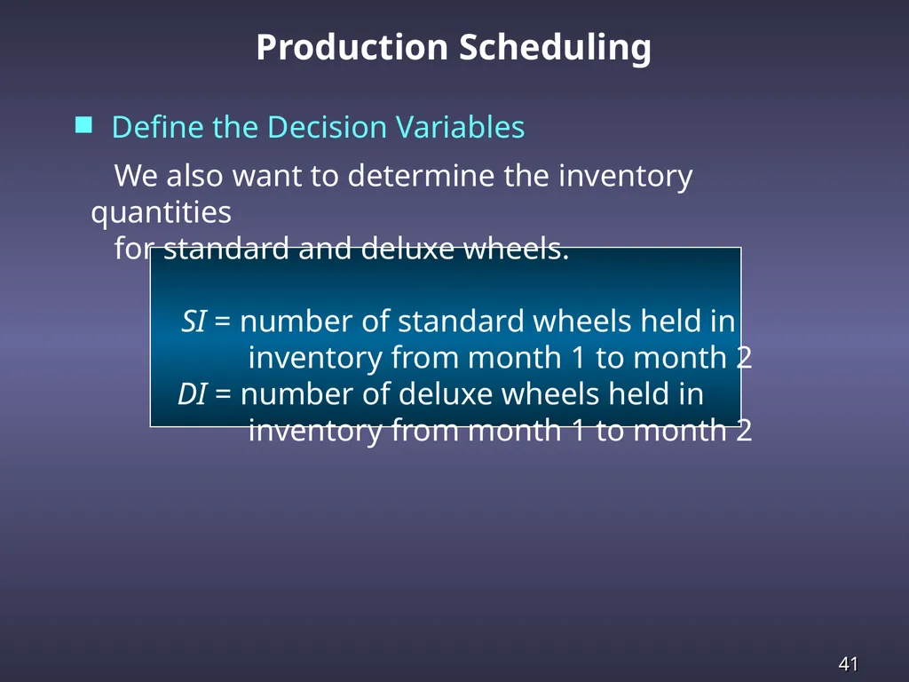
slide41. Production Scheduling We also want to determine the inventory quantities
for standard and deluxe wheels.
SI = number of standard wheels held in
inventory from month 1 to month 2
DI = number of deluxe wheels held in
inventory from month 1 to month 2 Define the Decision Variables<br>
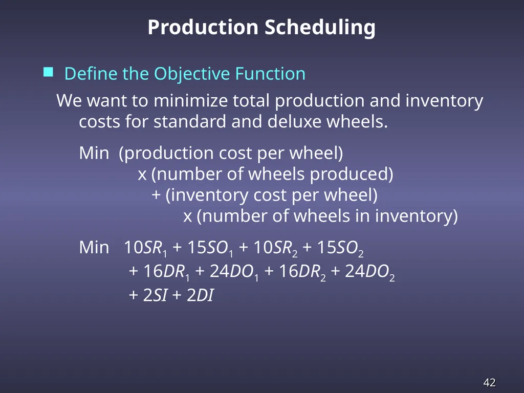
slide42. Production Scheduling We want to minimize total production and inventory costs for standard and deluxe wheels.
Min (production cost per wheel)
x (number of wheels produced)
+ (inventory cost per wheel)
x (number of wheels in inventory)
Min 10SR1 + 15SO1 + 10SR2 + 15SO2
+ 16DR1 + 24DO1 + 16DR2 + 24DO2
+ 2SI + 2DI Define the Objective Function<br>
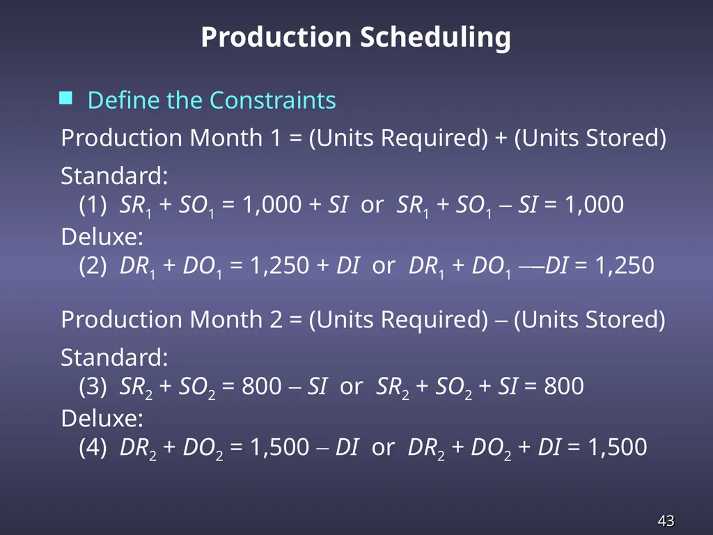
slide43. Production Scheduling Production Month 1 = (Units Required) + (Units Stored)
Standard:
(1) SR1 + SO1 = 1,000 + SI or SR1 + SO1 - SI = 1,000
Deluxe:
(2) DR1 + DO1 = 1,250 + DI or DR1 + DO1 -–DI = 1,250
Production Month 2 = (Units Required) - (Units Stored)
Standard:
(3) SR2 + SO2 = 800 - SI or SR2 + SO2 + SI = 800
Deluxe:
(4) DR2 + DO2 = 1,500 - DI or DR2 + DO2 + DI = 1,500 Define the Constraints<br>
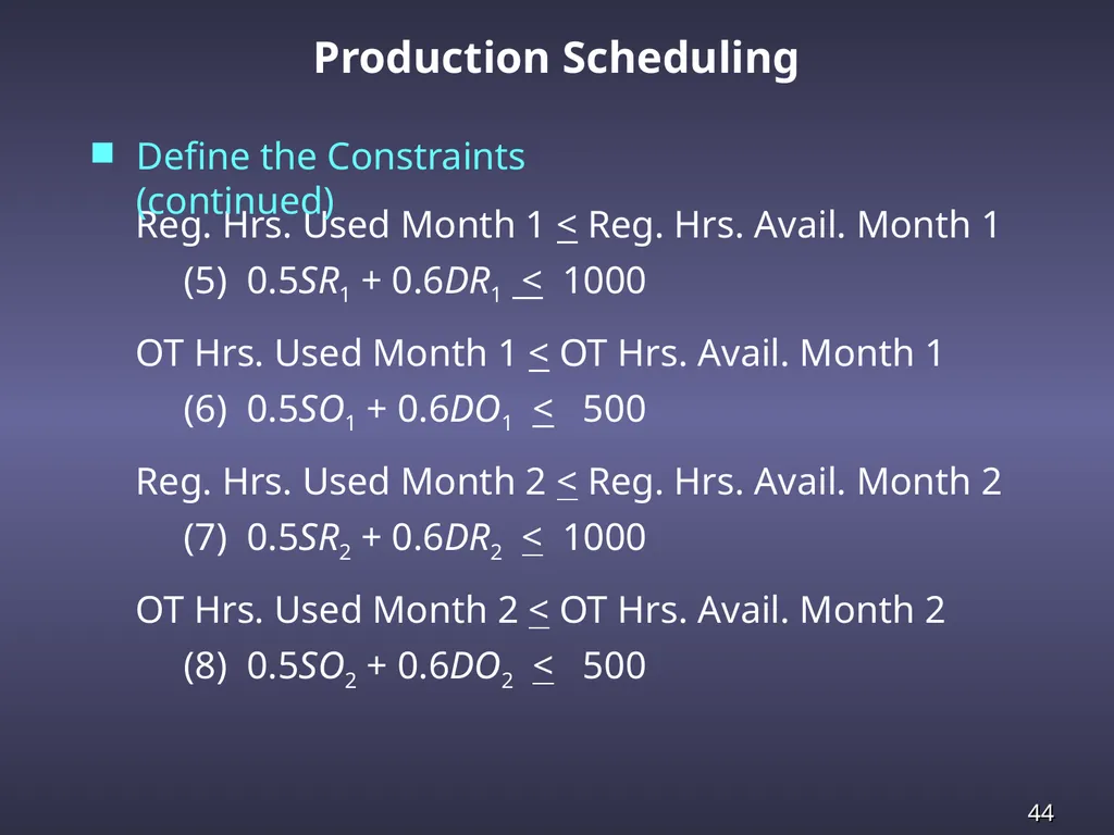
slide44. Production Scheduling Reg. Hrs. Used Month 1 < Reg. Hrs. Avail. Month 1
(5) 0.5SR1 + 0.6DR1 < 1000
OT Hrs. Used Month 1 < OT Hrs. Avail. Month 1
(6) 0.5SO1 + 0.6DO1 < 500
Reg. Hrs. Used Month 2 < Reg. Hrs. Avail. Month 2
(7) 0.5SR2 + 0.6DR2 < 1000
OT Hrs. Used Month 2 < OT Hrs. Avail. Month 2
(8) 0.5SO2 + 0.6DO2 < 500 Define the Constraints (continued)<br>
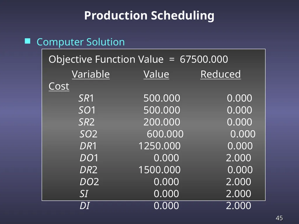
slide45. Objective Function Value = 67500.000
Variable Value Reduced Cost
SR1 500.000 0.000
SO1 500.000 0.000
SR2 200.000 0.000
SO2 600.000 0.000
DR1 1250.000 0.000
DO1 0.000 2.000
DR2 1500.000 0.000
DO2 0.000 2.000
SI 0.000 2.000
DI 0.000 2.000 Computer Solution Production Scheduling<br>
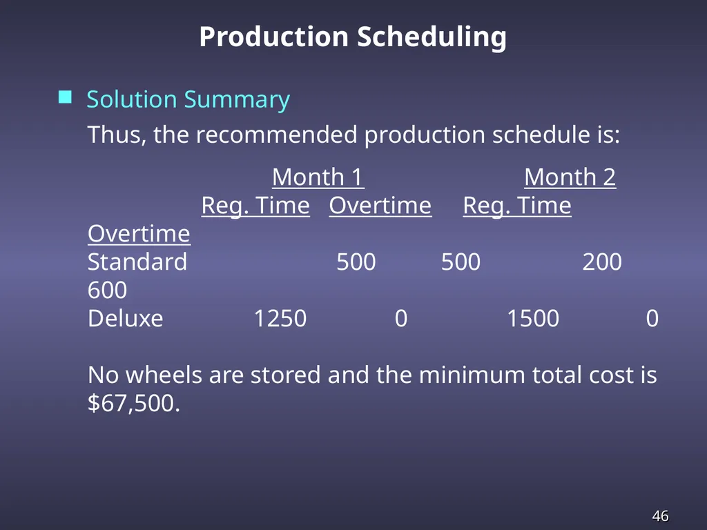
slide46. Thus, the recommended production schedule is:
Month 1 Month 2
Reg. Time Overtime Reg. Time Overtime
Standard 500 500 200 600
Deluxe 1250 0 1500 0
No wheels are stored and the minimum total cost is $67,500. Solution Summary Production Scheduling<br>
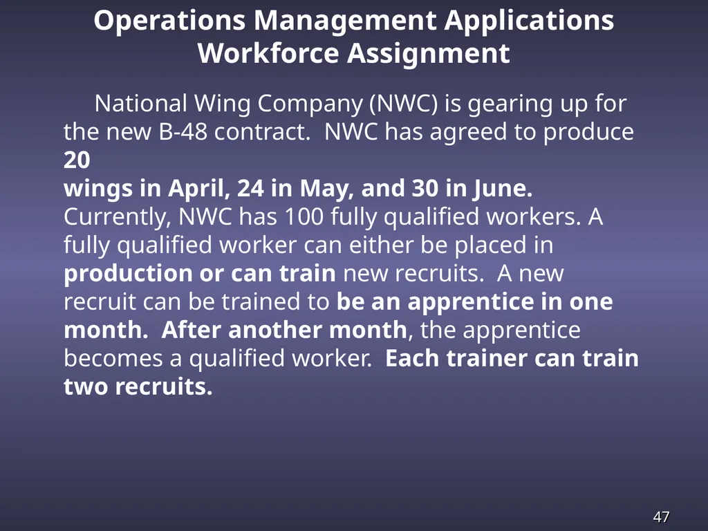
slide47. Operations Management Applications
Workforce Assignment National Wing Company (NWC) is gearing up for
the new B-48 contract. NWC has agreed to produce 20
wings in April, 24 in May, and 30 in June. Currently, NWC has 100 fully qualified workers. A fully qualified worker can either be placed in production or can train new recruits. A new recruit can be trained to be an apprentice in one month. After another month, the apprentice becomes a qualified worker. Each trainer can train two recruits.<br>
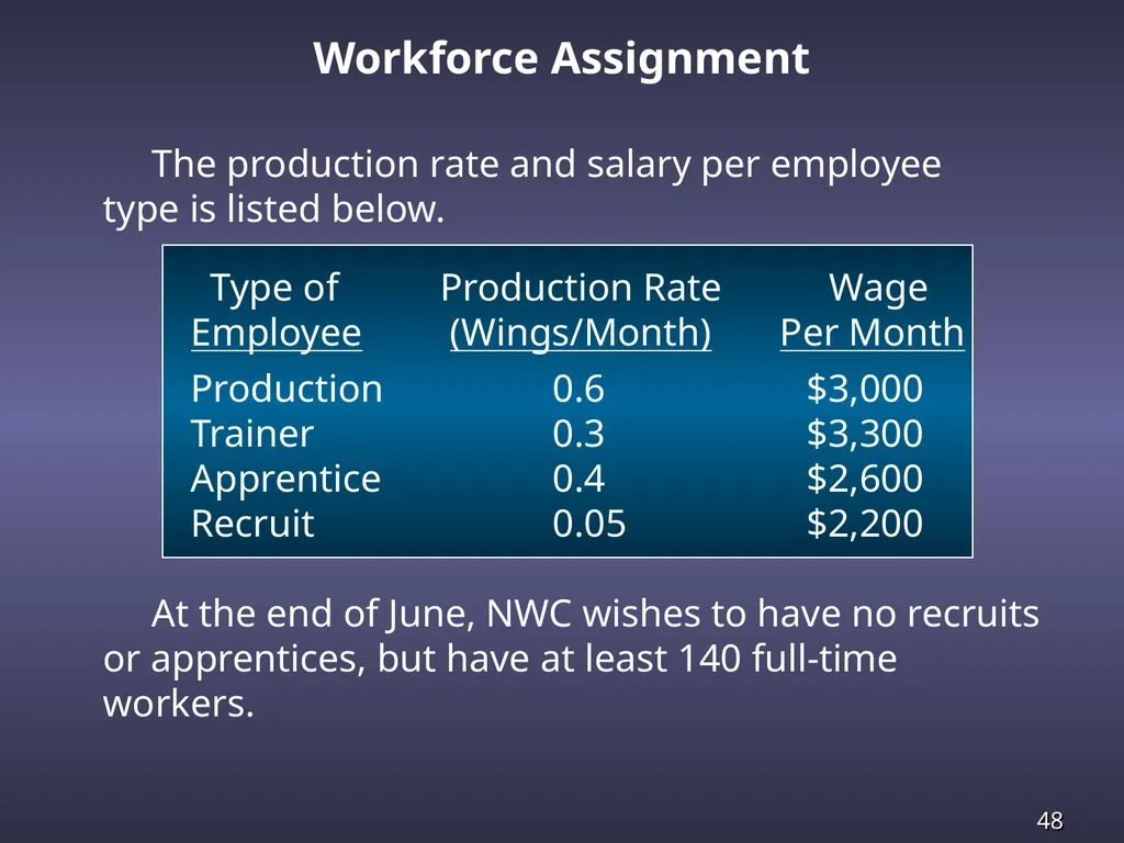
slide48. Workforce Assignment The production rate and salary per employee
type is listed below.
Type of Production Rate Wage
Employee (Wings/Month) Per Month
Production 0.6 $3,000
Trainer 0.3 $3,300
Apprentice 0.4 $2,600
Recruit 0.05 $2,200
At the end of June, NWC wishes to have no recruits
or apprentices, but have at least 140 full-time workers.<br>
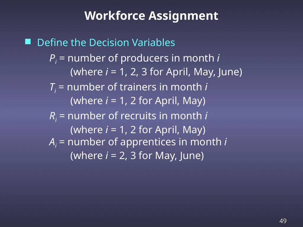
slide49. Workforce Assignment Define the Decision Variables Pi = number of producers in month i
(where i = 1, 2, 3 for April, May, June)
Ti = number of trainers in month i
(where i = 1, 2 for April, May)
Ri = number of recruits in month i
(where i = 1, 2 for April, May)
Ai = number of apprentices in month i
(where i = 2, 3 for May, June)<br>
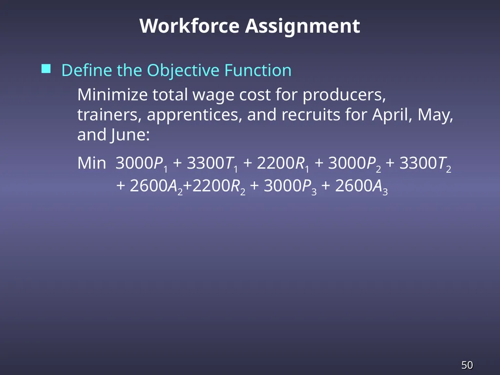
slide50. Workforce Assignment Define the Objective Function Minimize total wage cost for producers, trainers, apprentices, and recruits for April, May, and June:
Min 3000P1 + 3300T1 + 2200R1 + 3000P2 + 3300T2
+ 2600A2+2200R2 + 3000P3 + 2600A3<br>
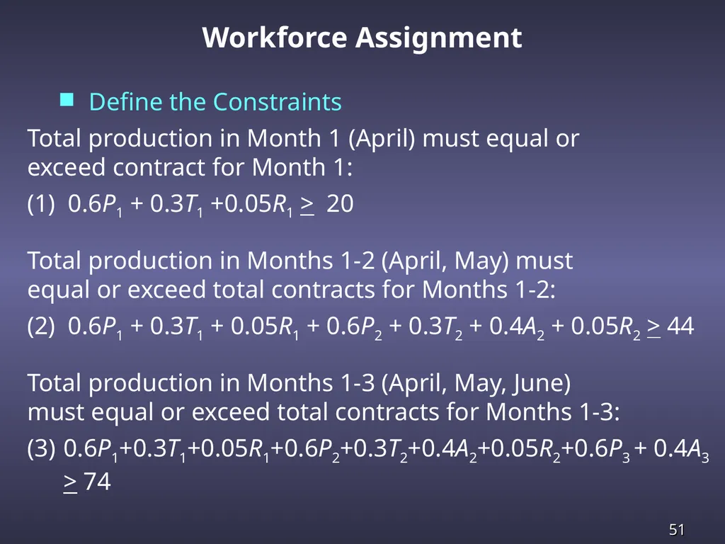
slide51. Workforce Assignment Define the Constraints Total production in Month 1 (April) must equal or
exceed contract for Month 1:
(1) 0.6P1 + 0.3T1 +0.05R1 > 20
Total production in Months 1-2 (April, May) must
equal or exceed total contracts for Months 1-2:
(2) 0.6P1 + 0.3T1 + 0.05R1 + 0.6P2 + 0.3T2 + 0.4A2 + 0.05R2 > 44
Total production in Months 1-3 (April, May, June)
must equal or exceed total contracts for Months 1-3:
0.6P1+0.3T1+0.05R1+0.6P2+0.3T2+0.4A2+0.05R2+0.6P3 + 0.4A3 > 74<br>
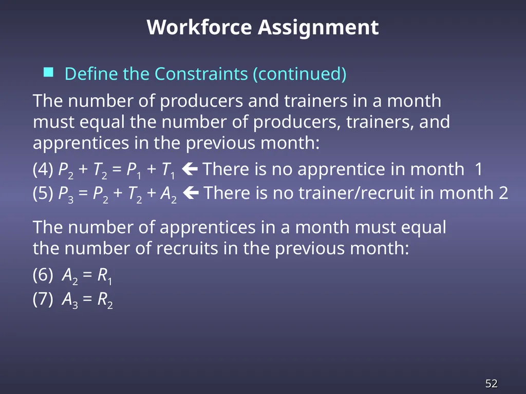
slide52. Workforce Assignment Define the Constraints (continued) The number of producers and trainers in a month
must equal the number of producers, trainers, and
apprentices in the previous month:
(4) P2 + T2 = P1 + T1 There is no apprentice in month 1
(5) P3 = P2 + T2 + A2 There is no trainer/recruit in month 2
The number of apprentices in a month must equal
the number of recruits in the previous month:
(6) A2 = R1
(7) A3 = R2<br>
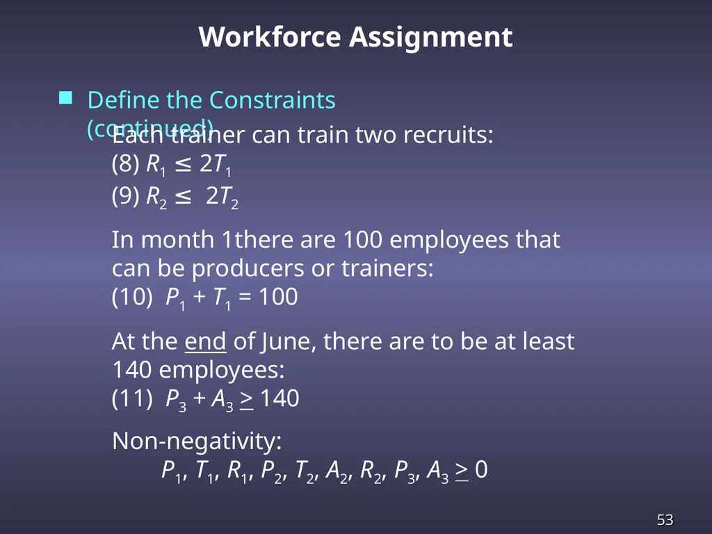
slide53. Workforce Assignment Define the Constraints (continued) Each trainer can train two recruits:
(8) R1 ≤ 2T1
(9) R2 ≤ 2T2
In month 1there are 100 employees that can be producers or trainers:
(10) P1 + T1 = 100
At the end of June, there are to be at least 140 employees:
(11) P3 + A3 > 140
Non-negativity:
P1, T1, R1, P2, T2, A2, R2, P3, A3 > 0<br>
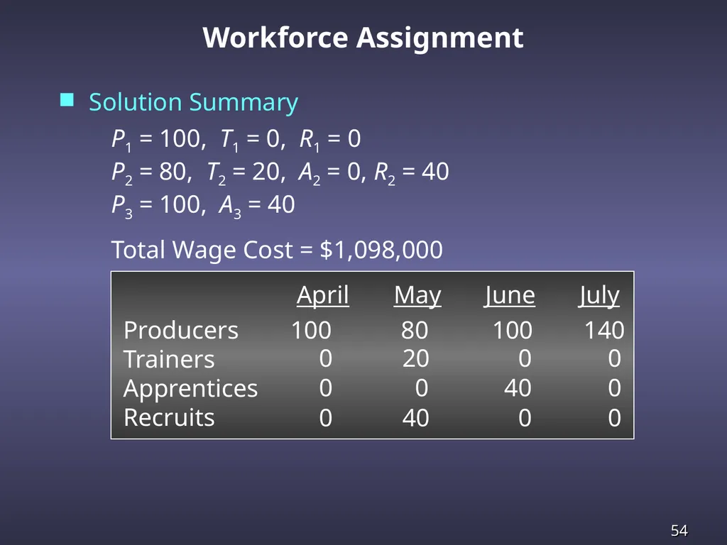
slide54. Workforce Assignment Solution Summary P1 = 100, T1 = 0, R1 = 0
P2 = 80, T2 = 20, A2 = 0, R2 = 40
P3 = 100, A3 = 40
Total Wage Cost = $1,098,000 Producers
Trainers
Apprentices
Recruits April May June July 100 80 100 140 0 20 0 0 0 0 40 0 0 40 0 0<br>
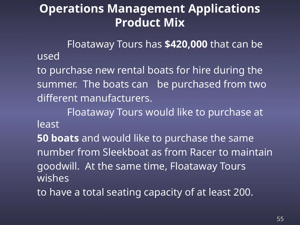
slide55. Operations Management Applications Product Mix Floataway Tours has $420,000 that can be used
to purchase new rental boats for hire during the
summer. The boats can be purchased from two
different manufacturers.
Floataway Tours would like to purchase at least
50 boats and would like to purchase the same
number from Sleekboat as from Racer to maintain
goodwill. At the same time, Floataway Tours wishes
to have a total seating capacity of at least 200.<br>
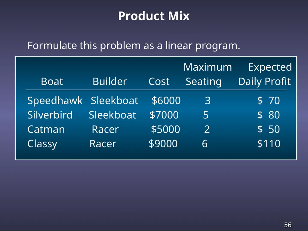
slide56. Formulate this problem as a linear program.
Maximum Expected
Boat Builder Cost Seating Daily Profit
Speedhawk Sleekboat $6000 3 $ 70
Silverbird Sleekboat $7000 5 $ 80
Catman Racer $5000 2 $ 50
Classy Racer $9000 6 $110 Product Mix<br>
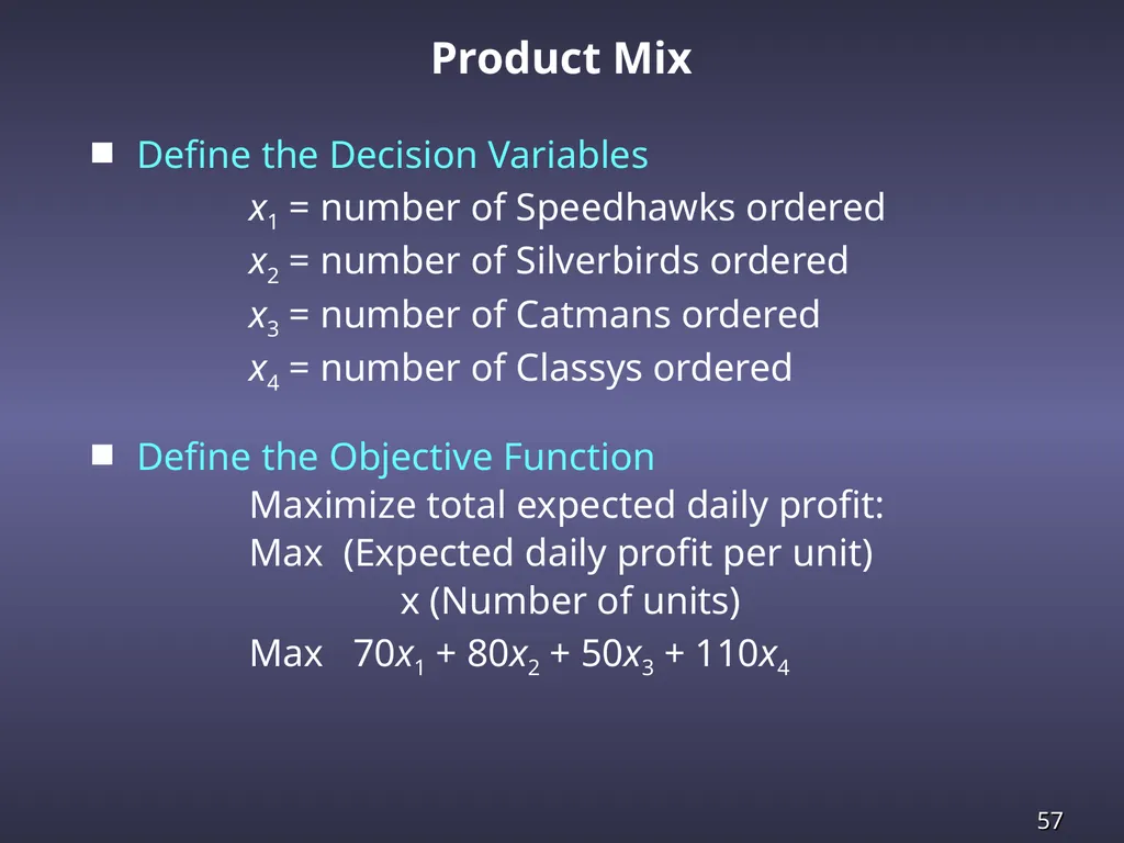
slide57. Define the Decision Variables
x1 = number of Speedhawks ordered
x2 = number of Silverbirds ordered
x3 = number of Catmans ordered
x4 = number of Classys ordered
Define the Objective Function
Maximize total expected daily profit:
Max (Expected daily profit per unit)
x (Number of units)
Max 70x1 + 80x2 + 50x3 + 110x4 Product Mix<br>
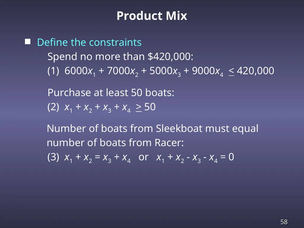
slide58. Define the constraints
Spend no more than $420,000:
(1) 6000x1 + 7000x2 + 5000x3 + 9000x4 < 420,000
Purchase at least 50 boats:
(2) x1 + x2 + x3 + x4 > 50
Number of boats from Sleekboat must equal
number of boats from Racer:
(3) x1 + x2 = x3 + x4 or x1 + x2 - x3 - x4 = 0 Product Mix<br>
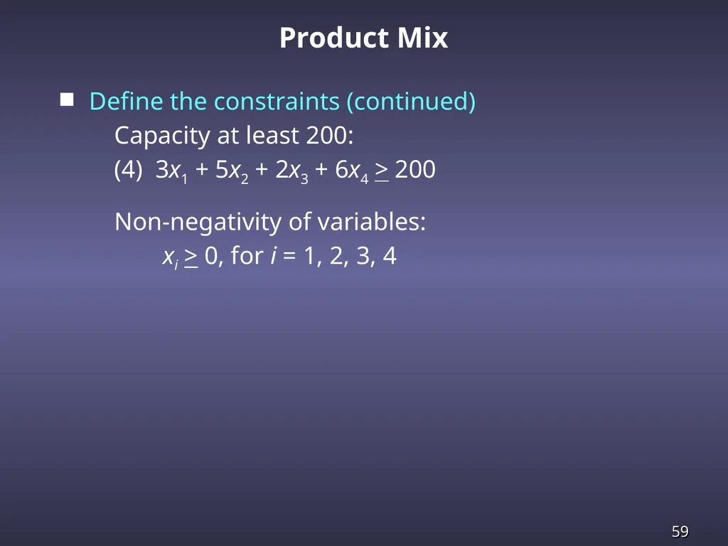
slide59. Define the constraints (continued)
Capacity at least 200:
(4) 3x1 + 5x2 + 2x3 + 6x4 > 200
Non-negativity of variables:
xi > 0, for i = 1, 2, 3, 4 Product Mix<br>
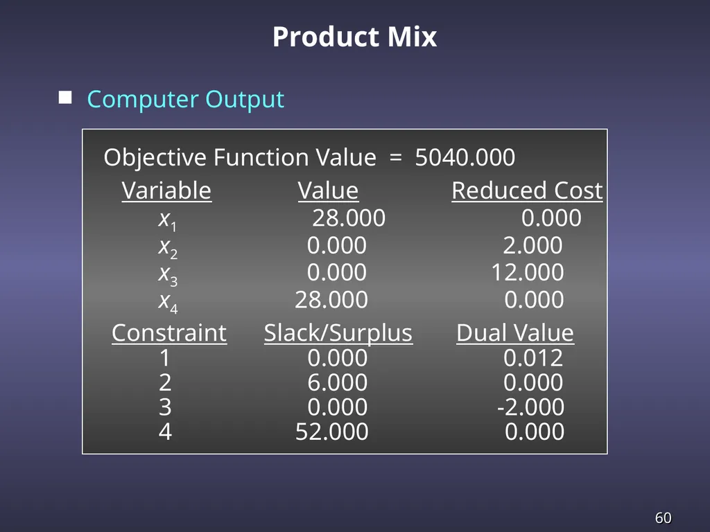
slide60. Computer Output
Objective Function Value = 5040.000
Variable Value Reduced Cost
x1 28.000 0.000
x2 0.000 2.000
x3 0.000 12.000
x4 28.000 0.000
Constraint Slack/Surplus Dual Value
1 0.000 0.012
2 6.000 0.000
3 0.000 -2.000
4 52.000 0.000 Product Mix<br>
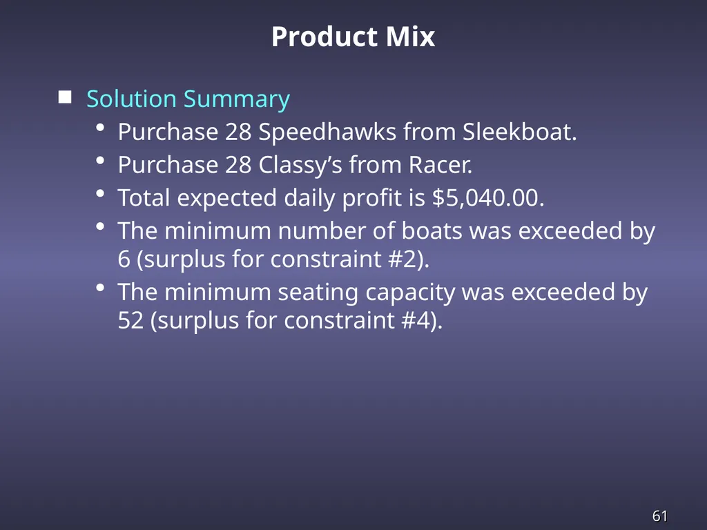
slide61. Solution Summary
Purchase 28 Speedhawks from Sleekboat.
Purchase 28 Classy’s from Racer.
Total expected daily profit is $5,040.00.
The minimum number of boats was exceeded by 6 (surplus for constraint #2).
The minimum seating capacity was exceeded by 52 (surplus for constraint #4). Product Mix<br>
slide62. Operations Management Applications Blending Problem Ferdinand Feed Company receives four raw
grains from which it blends its dry pet food. The pet
food advertises that each 8-ounce packet meets the
minimum daily requirements for vitamin C, protein
and iron. The cost of each raw grain as well as the
vitamin C, protein, and iron units per pound of each
grain are summarized on the next slide.<br>
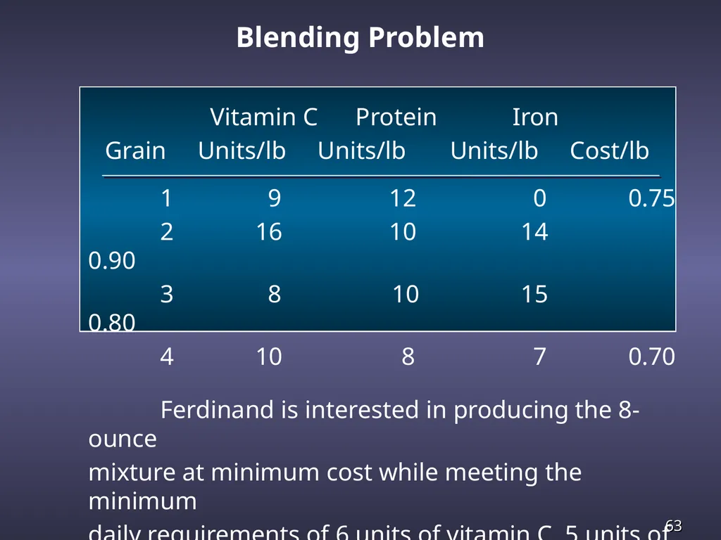
slide63. Blending Problem Vitamin C Protein Iron
Grain Units/lb Units/lb Units/lb Cost/lb
1 9 12 0 0.75
2 16 10 14 0.90
3 8 10 15 0.80
4 10 8 7 0.70
Ferdinand is interested in producing the 8-ounce
mixture at minimum cost while meeting the minimum
daily requirements of 6 units of vitamin C, 5 units of
protein, and 5 units of iron.<br>
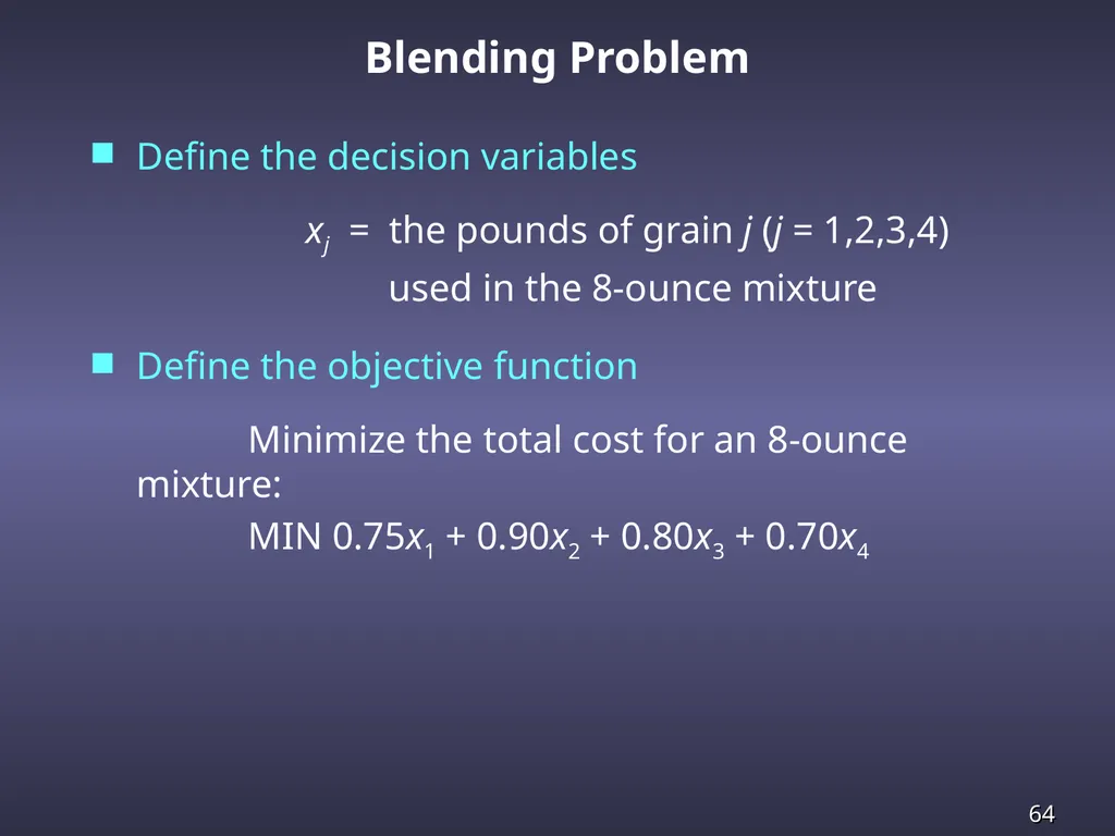
slide64. Blending Problem Define the decision variables
xj = the pounds of grain j (j = 1,2,3,4)
used in the 8-ounce mixture
Define the objective function
Minimize the total cost for an 8-ounce mixture:
MIN 0.75x1 + 0.90x2 + 0.80x3 + 0.70x4<br>
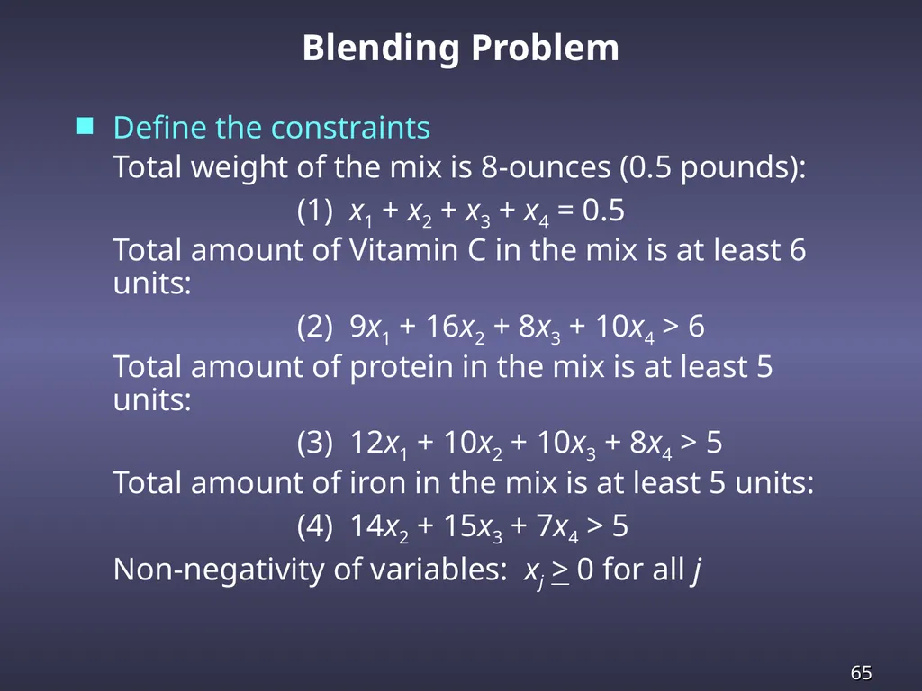
slide65. Blending Problem Define the constraints
Total weight of the mix is 8-ounces (0.5 pounds):
(1) x1 + x2 + x3 + x4 = 0.5
Total amount of Vitamin C in the mix is at least 6 units:
(2) 9x1 + 16x2 + 8x3 + 10x4 > 6
Total amount of protein in the mix is at least 5 units:
(3) 12x1 + 10x2 + 10x3 + 8x4 > 5
Total amount of iron in the mix is at least 5 units:
(4) 14x2 + 15x3 + 7x4 > 5
Non-negativity of variables: xj > 0 for all j<br>
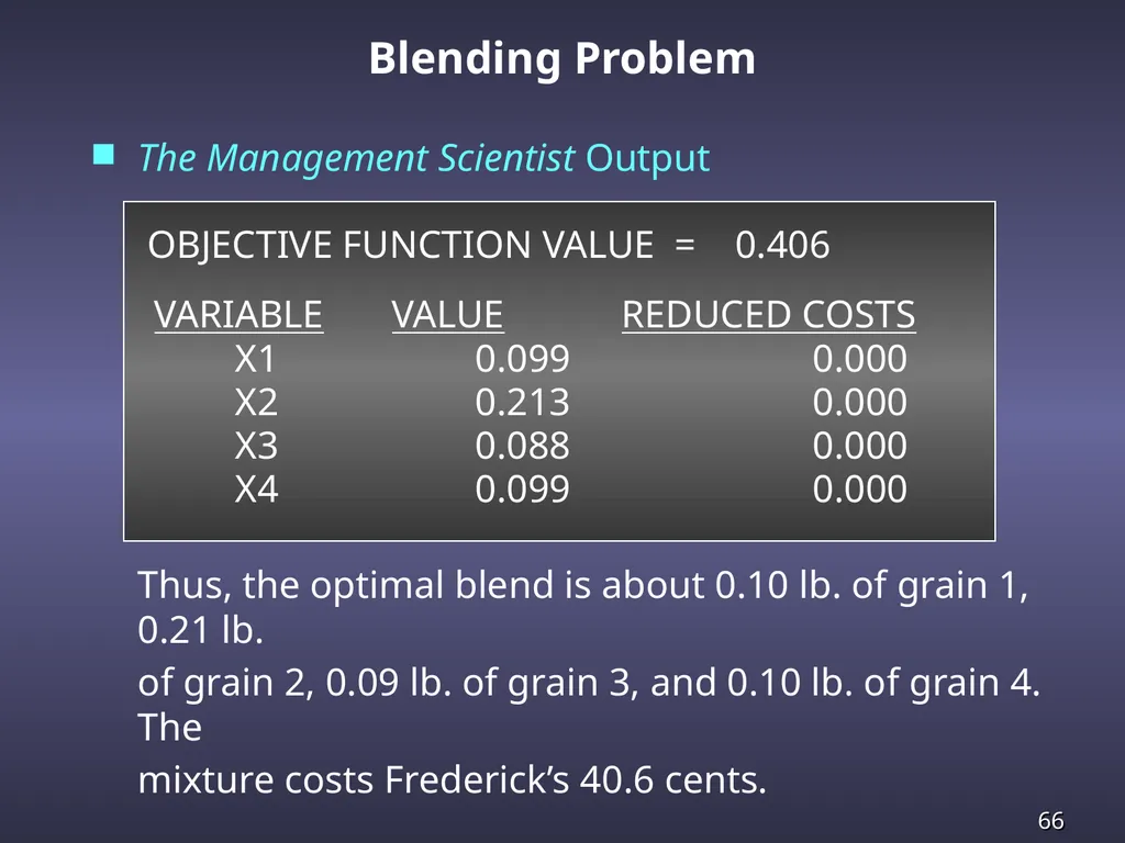
slide66. The Management Scientist Output
OBJECTIVE FUNCTION VALUE = 0.406
VARIABLE VALUE REDUCED COSTS
X1 0.099 0.000
X2 0.213 0.000
X3 0.088 0.000
X4 0.099 0.000
Thus, the optimal blend is about 0.10 lb. of grain 1, 0.21 lb.
of grain 2, 0.09 lb. of grain 3, and 0.10 lb. of grain 4. The
mixture costs Frederick’s 40.6 cents. Blending Problem<br>
slide67. End of Chapter 4<br>
A. Asef-Vaziri<br>
slide2. Chapter 4 Linear Programming Applications in Marketing, Finance, and Operations Marketing Applications
Financial Applications
Operations Management Applications<br>
slide3. Marketing Applications: Media Selection SMM Company recently developed a new instant
salad machine, has $282,000 to spend on advertising. The product is to be initially test marketed in the Dallas
area. The money is to be spent on a TV advertising blitz
during one weekend (Friday, Saturday, and Sunday) in
November. The three options available are: daytime advertising,
evening news advertising, and Sunday game-time
advertising. A mixture of one-minute TV spots is desired.<br>
slide4. Media Selection Estimated Audience
Ad Type Reached With Each Ad Cost Per Ad
Daytime 3,000 $5,000
Evening News 4,000 $7,000
Sunday Game 75,000 $100,000 SMM wants to take out at least one ad of each type (daytime, evening-news, and game-time). Further, there are only two game-time ad spots available. There are ten daytime spots and six evening news spots available daily. SMM wants to have at least 5 ads per day, but spend no more than $50,000 on Friday and no more than $75,000 on Saturday.<br>
slide5. Media Selection DFR = number of daytime ads on Friday
DSA = number of daytime ads on Saturday
DSU = number of daytime ads on Sunday
EFR = number of evening ads on Friday
ESA = number of evening ads on Saturday
ESU = number of evening ads on Sunday
GSU = number of game-time ads on Sunday Define the Decision Variables<br>
slide6. Media Selection Define the Objective Function Maximize the total audience reached:
Max (audience reached per ad of each type)
x (number of ads used of each type)
Max 3000DFR +3000DSA +3000DSU +4000EFR
+4000ESA +4000ESU +75000GSU<br>
slide7. Media Selection Define the Constraints At least one ad of each type (daytime, evening-news, and game-time).
(1) DFR + DSA + DSU > 1
(2) EFR + ESA + ESU > 1
(3) GSU > 1
There are ten daytime spots available daily.
(4) DFR < 10
(5) DSA < 10
(6) DSU < 10
There are six evening news spots available daily.
(7) EFR < 6
(8) ESA < 6
(9) ESU < 6<br>
slide8. Media Selection Define the Constraints (continued) Only two Sunday game-time ad spots available:
(10) GSU < 2
At least 5 ads per day:
(11) DFR + EFR > 5
(12) DSA + ESA > 5
(13) DSU + ESU + GSU > 5
Spend no more than $50,000 on Friday:
(14) 5000DFR + 7000EFR < 50000<br>
slide9. Media Selection Define the Constraints (continued) Spend no more than $75,000 on Saturday:
(15) 5000DSA + 7000ESA < 75000
Spend no more than $282,000 in total:
(16) 5000DFR + 5000DSA + 5000DSU + 7000EFR
+ 7000ESA + 7000ESU + 100000GSU7 < 282000
Non-negativity:
DFR, DSA, DSU, EFR, ESA, ESU, GSU > 0<br>
slide10. Media Selection The Management Scientist Solution<br>
slide11. A firm conducts marketing research to learn about consumer characteristics, attitudes, and preferences.
Marketing research services include designing the study, conducting surveys, analyzing data collected, and providing recommendations for the client.
In the research design phase, targets or quotas may be established for the number and types of respondents to be surveyed.
The marketing research firm’s objective is to conduct the survey so as to meet the client’s needs at a minimum cost. Marketing Applications<br>
slide12. Marketing Research: Marketing Research Market Survey, Inc. (MSI) specializes in evaluating consumer reaction to new products, services, and advertising campaigns. A client firm requested MSI’s assistance in ascertaining consumer reaction to a recently marketed household product.
During meetings with the client, MSI agreed to conduct door-to-door personal interviews to obtain responses from households with children and households without children. In addition, MSI agreed to conduct both day and evening interviews.<br>
slide13. Marketing Research The client’s contract called for MSI to conduct 1000 interviews under the following quota guidelines:
Interview at least 400 households with children.
2. Interview at least 400 households without children.
3. The total number of households interviewed during the
evening must be at least as great as the number of
households interviewed during the day.
4. At least 40% of the interviews for households with
children must be conducted during the evening.
5. At least 60% of the interviews for households without
children must be conducted during the evening.<br>
slide14. Marketing Research Because the interviews for households with children take additional interviewer time and because evening interviewers are paid more than daytime interviewers, the cost varies with the type of interview. Based on previous research studies, estimates of the interview costs are as follows:
Interview Cost
Household Day Evening
Children $20 $25
No children $18 $20<br>
slide15. Marketing Research In formulating the linear programming model for the MSI problem, we utilize the following decision-variable notation:
DC = the number of daytime interviews of households
with children
EC = the number of evening interviews of households
with children
DNC = the number of daytime interviews of households
without children
ENC = the number of evening interviews of households
without children<br>
slide16. Marketing Research The objective function: conduct the survey so as to meet the client’s needs at a minimum cost.
Min 20DC + 25EC + 18DNC + 20ENC
Conduct 1000 interviews under
DC + EC + DNC + ENC = 1000
It really does not matter if we write
DC + EC + DNC + ENC > 1000
Why
Interview at least 400 households with children.
DC + EC > 400
Interview at least 400 households without children
DNC + ENC > 400<br>
slide17. Marketing Research The total number of households interviewed during the evening must be at least as great as the number of households interviewed during the day.
EC + ENC > DC + DNC or -DC + EC - DNC + ENC > 0
At least 40% of the interviews for households with children must be conducted during the evening.
EC > 0.4(DC + EC) or -0.4DC + 0.6EC > 0
At least 60% of the interviews for households without children must be conducted during the evening.
ENC > 0.6(DNC + ENC) or -0.6DNC + 0.4ENC > 0
The non-negativity requirements: DC, EC, DNC, ENC > 0<br>
slide18. Marketing Research The 4-variable, 6-constraint LP problem formulation is:<br>
slide19. Marketing Research<br>
slide20. Financial Applications: Portfolio Selection Winslow Savings has $20 million available for
investment. It wishes to invest over the next four
months in such a way that it will maximize the total
interest earned over the four month period as well as
have at least $10 million available at the start of the
fifth month for a high rise building venture in which it
will be participating.<br>
slide21. Portfolio Selection For the time being, Winslow wishes to invest
only in 2-month government bonds (earning 2% over
the 2-month period) and 3-month construction loans
(earning 6% over the 3-month period). Each of these
is available each month for investment. Funds not
invested in these two investments are liquid and earn
3/4 of 1% per month when invested locally.<br>
slide22. Portfolio Selection Formulate a linear program that will help
Winslow Savings determine how to invest over the
next four months if at no time does it wish to have
more than $8 million in either government bonds or
construction loans.<br>
slide23. Portfolio Selection Define the Decision Variables
Gi = amount of new investment in government
bonds in month i (for i = 1, 2, 3, 4)
Ci = amount of new investment in construction
loans in month i (for i = 1, 2, 3, 4)
Li = amount invested locally in month i,
(for i = 1, 2, 3, 4)<br>
slide24. Portfolio Selection Define the Objective Function
Maximize total interest earned in the 4-month period:
Max (interest rate on investment) X (amount invested)
Max 0.02G1 + 0.02G2 + 0.02G3 + 0.02G4
+ 0.06C1 + 0.06C2 + 0.06C3 + 0.06C4
+ 0.0075L1 + 0.0075L2 + 0.0075L3 + 0.0075L4<br>
slide25. Portfolio Selection Define the Constraints
Month 1's total investment limited to $20 million:
(1) G1 + C1 + L1 = 20,000,000
Month 2's total investment limited to principle and interest invested locally in Month 1:
(2) G2 + C2 + L2 = 1.0075L1
or G2 + C2 - 1.0075L1 + L2 = 0<br>
slide26. Portfolio Selection Define the Constraints (continued)
Month 3's total investment amount limited to principle and interest invested in government bonds in Month 1 and locally invested in Month 2:
(3) G3 + C3 + L3 = 1.02G1 + 1.0075L2
or - 1.02G1 + G3 + C3 - 1.0075L2 + L3 = 0<br>
slide27. Portfolio Selection Define the Constraints (continued)
Month 4's total investment limited to principle and interest invested in construction loans in Month 1, goverment bonds in Month 2, and locally invested in Month 3:
(4) G4 + C4 + L4 = 1.06C1 + 1.02G2 + 1.0075L3
or - 1.02G2 + G4 - 1.06C1 + C4 - 1.0075L3 + L4 = 0
$10 million must be available at start of Month 5:
(5) 1.06C2 + 1.02G3 + 1.0075L4 > 10,000,000<br>
slide28. Portfolio Selection Define the Constraints (continued)
No more than $8 million in government bonds at any time:
(6) G1 < 8,000,000
(7) G1 + G2 < 8,000,000
(8) G2 + G3 < 8,000,000
(9) G3 + G4 < 8,000,000<br>
slide29. Portfolio Selection Define the Constraints (continued)
No more than $8 million in construction loans at any time:
(10) C1 < 8,000,000
(11) C1 + C2 < 8,000,000
(12) C1 + C2 + C3 < 8,000,000
(13) C2 + C3 + C4 < 8,000,000
Non-negativity:
Gi, Ci, Li > 0 for i = 1, 2, 3, 4<br>
slide30. Portfolio Selection Computer Solution<br>
slide31. Financial Planning Hewlitt Corporation established an early retirement program as part of its corporate restructuring. At the close of the voluntary sign-up period, 68 employees had elected early retirement. As a result of these early retirements, the company incurs the following obligations over the next eight years:
Year 1 2 3 4 5 6 7 8
Cash
Required 430 210 222 231 240 195 225 255
The cash requirements (in thousands of dollars) are due at the beginning of each year.<br>
slide32. Financial Planning The corporate treasurer must determine how much money must be set aside today to meet the eight yearly financial obligations as they come due. The financing plan for the retirement program includes investments in government bonds as well as savings. The investments in government bonds are limited to three choices:
Years to
Bond Price Rate (%) Maturity
1 $1150 8.875 5
2 1000 5.500 6
3 1350 11.750 7<br>
slide33. Financial Planning The government bonds have a par value of $1000, which means that even with different prices each bond pays $1000 at maturity. The rates shown are based on the par value. For purposes of planning, the treasurer assumed that any funds not invested in bonds will be placed in savings and earn interest at an annual rate of 4%.<br>
slide34. Financial Planning Define the Decision Variables
F = total dollars required to meet the retirement plan’s eight-year obligation
B1 = units of bond 1 purchased at the beginning of year 1
B2 = units of bond 2 purchased at the beginning of year 1
B3 = units of bond 3 purchased at the beginning of year 1
S = amount placed in savings at the beginning of year i for i = 1, . . . , 8<br>
slide35. Financial Planning Define the Objective Function
The objective function is to minimize the total dollars needed to meet the retirement plan’s eight-year obligation: Min F
Define the Constraints
A key feature of this type of financial planning problem is that a constraint must be formulated for each year of the planning horizon. It’s form is:
(Funds available at the beginning of the year)
- (Funds invested in bonds and placed in savings)
= (Cash obligation for the current year)<br>
slide36. Financial Planning Define the Constraints
A constraint must be formulated for each year of the planning horizon in the following form:
Year 1: F – 1.15B1 – 1B2 – 1.35B3 – S1 = 430
Year 2: 0.08875B1 + 0.055B2 + 0.1175B3 + 1.04S1 - S2 = 210
Year 3: 0.08875B1 + 0.055B2 + 0.1175B3 + 1.04S2 – S3 = 222
Year 4: 0.08875B1 + 0.055B2 + 0.1175B3 + 1.04S3 – S4 = 231
Year 5: 0.08875B1 + 0.055B2 + 0.1175B3 + 1.04S4 – S5 = 240
Year 6 1.08875B1 + 0.055B2 + 0.1175B3 + 1.04S5 – S6 = 195
Year 7: 1.055B2 + 0.1175B3 + 1.04S6 – S7 = 225
Year 8: 1.1175B3 + 1.04S7 – S8 = 255<br>
slide37. Financial Planning Optimal solution to the 12-variable, 8-constraint LP problem:
Minimum total obligation = $1,728,794
Bond Units Purchased Investment Amount
1 B1 = 144.988 $1150(144.988) = $166,736
2 B2 = 187.856 $1000(187.856) = $187,856
3 B3 = 228.188 $1350(228.188) = $308,054<br>
slide38. Operations Management Applications LP can be used in operations management to aid in decision-making about product mix, production scheduling, staffing, inventory control, capacity planning, and other issues.
An important application of LP is multi-period planning such as production scheduling.
Usually the objective is to establish an efficient, low-cost production schedule for one or more products over several time periods.
Typical constraints include limitations on production capacity, labor capacity, storage space, and more.<br>
slide39. Chip Hoose is the owner of Hoose Custom Wheels. Chip has just received orders for 1,000 standard wheels
and 1,250 deluxe wheels next month and for 800 standard and 1,500 deluxe the following month. All
orders must be filled. Operations Management Applications
Production Scheduling The cost of making standard wheels is $10 and deluxe
wheels is $16. Overtime rates are 50% higher. There
are 1,000 hours of regular time and 500 hours of overtime available each month. It takes 0.5 hour to make a standard wheel and 0.6 hour to make a deluxe wheel.
The cost of storing a wheel from one month to the next is $2.<br>
slide40. Production Scheduling We want to determine the regular-time and overtime
production quantities in each month for standard and
deluxe wheels.
Month 1 Month 2
Wheel Reg. Time Overtime Reg. Time Overtime
Standard SR1 SO1 SR2 SO2
Deluxe DR1 DO1 DR2 DO2 Define the Decision Variables<br>
slide41. Production Scheduling We also want to determine the inventory quantities
for standard and deluxe wheels.
SI = number of standard wheels held in
inventory from month 1 to month 2
DI = number of deluxe wheels held in
inventory from month 1 to month 2 Define the Decision Variables<br>
slide42. Production Scheduling We want to minimize total production and inventory costs for standard and deluxe wheels.
Min (production cost per wheel)
x (number of wheels produced)
+ (inventory cost per wheel)
x (number of wheels in inventory)
Min 10SR1 + 15SO1 + 10SR2 + 15SO2
+ 16DR1 + 24DO1 + 16DR2 + 24DO2
+ 2SI + 2DI Define the Objective Function<br>
slide43. Production Scheduling Production Month 1 = (Units Required) + (Units Stored)
Standard:
(1) SR1 + SO1 = 1,000 + SI or SR1 + SO1 - SI = 1,000
Deluxe:
(2) DR1 + DO1 = 1,250 + DI or DR1 + DO1 -–DI = 1,250
Production Month 2 = (Units Required) - (Units Stored)
Standard:
(3) SR2 + SO2 = 800 - SI or SR2 + SO2 + SI = 800
Deluxe:
(4) DR2 + DO2 = 1,500 - DI or DR2 + DO2 + DI = 1,500 Define the Constraints<br>
slide44. Production Scheduling Reg. Hrs. Used Month 1 < Reg. Hrs. Avail. Month 1
(5) 0.5SR1 + 0.6DR1 < 1000
OT Hrs. Used Month 1 < OT Hrs. Avail. Month 1
(6) 0.5SO1 + 0.6DO1 < 500
Reg. Hrs. Used Month 2 < Reg. Hrs. Avail. Month 2
(7) 0.5SR2 + 0.6DR2 < 1000
OT Hrs. Used Month 2 < OT Hrs. Avail. Month 2
(8) 0.5SO2 + 0.6DO2 < 500 Define the Constraints (continued)<br>
slide45. Objective Function Value = 67500.000
Variable Value Reduced Cost
SR1 500.000 0.000
SO1 500.000 0.000
SR2 200.000 0.000
SO2 600.000 0.000
DR1 1250.000 0.000
DO1 0.000 2.000
DR2 1500.000 0.000
DO2 0.000 2.000
SI 0.000 2.000
DI 0.000 2.000 Computer Solution Production Scheduling<br>
slide46. Thus, the recommended production schedule is:
Month 1 Month 2
Reg. Time Overtime Reg. Time Overtime
Standard 500 500 200 600
Deluxe 1250 0 1500 0
No wheels are stored and the minimum total cost is $67,500. Solution Summary Production Scheduling<br>
slide47. Operations Management Applications
Workforce Assignment National Wing Company (NWC) is gearing up for
the new B-48 contract. NWC has agreed to produce 20
wings in April, 24 in May, and 30 in June. Currently, NWC has 100 fully qualified workers. A fully qualified worker can either be placed in production or can train new recruits. A new recruit can be trained to be an apprentice in one month. After another month, the apprentice becomes a qualified worker. Each trainer can train two recruits.<br>
slide48. Workforce Assignment The production rate and salary per employee
type is listed below.
Type of Production Rate Wage
Employee (Wings/Month) Per Month
Production 0.6 $3,000
Trainer 0.3 $3,300
Apprentice 0.4 $2,600
Recruit 0.05 $2,200
At the end of June, NWC wishes to have no recruits
or apprentices, but have at least 140 full-time workers.<br>
slide49. Workforce Assignment Define the Decision Variables Pi = number of producers in month i
(where i = 1, 2, 3 for April, May, June)
Ti = number of trainers in month i
(where i = 1, 2 for April, May)
Ri = number of recruits in month i
(where i = 1, 2 for April, May)
Ai = number of apprentices in month i
(where i = 2, 3 for May, June)<br>
slide50. Workforce Assignment Define the Objective Function Minimize total wage cost for producers, trainers, apprentices, and recruits for April, May, and June:
Min 3000P1 + 3300T1 + 2200R1 + 3000P2 + 3300T2
+ 2600A2+2200R2 + 3000P3 + 2600A3<br>
slide51. Workforce Assignment Define the Constraints Total production in Month 1 (April) must equal or
exceed contract for Month 1:
(1) 0.6P1 + 0.3T1 +0.05R1 > 20
Total production in Months 1-2 (April, May) must
equal or exceed total contracts for Months 1-2:
(2) 0.6P1 + 0.3T1 + 0.05R1 + 0.6P2 + 0.3T2 + 0.4A2 + 0.05R2 > 44
Total production in Months 1-3 (April, May, June)
must equal or exceed total contracts for Months 1-3:
0.6P1+0.3T1+0.05R1+0.6P2+0.3T2+0.4A2+0.05R2+0.6P3 + 0.4A3 > 74<br>
slide52. Workforce Assignment Define the Constraints (continued) The number of producers and trainers in a month
must equal the number of producers, trainers, and
apprentices in the previous month:
(4) P2 + T2 = P1 + T1 There is no apprentice in month 1
(5) P3 = P2 + T2 + A2 There is no trainer/recruit in month 2
The number of apprentices in a month must equal
the number of recruits in the previous month:
(6) A2 = R1
(7) A3 = R2<br>
slide53. Workforce Assignment Define the Constraints (continued) Each trainer can train two recruits:
(8) R1 ≤ 2T1
(9) R2 ≤ 2T2
In month 1there are 100 employees that can be producers or trainers:
(10) P1 + T1 = 100
At the end of June, there are to be at least 140 employees:
(11) P3 + A3 > 140
Non-negativity:
P1, T1, R1, P2, T2, A2, R2, P3, A3 > 0<br>
slide54. Workforce Assignment Solution Summary P1 = 100, T1 = 0, R1 = 0
P2 = 80, T2 = 20, A2 = 0, R2 = 40
P3 = 100, A3 = 40
Total Wage Cost = $1,098,000 Producers
Trainers
Apprentices
Recruits April May June July 100 80 100 140 0 20 0 0 0 0 40 0 0 40 0 0<br>
slide55. Operations Management Applications Product Mix Floataway Tours has $420,000 that can be used
to purchase new rental boats for hire during the
summer. The boats can be purchased from two
different manufacturers.
Floataway Tours would like to purchase at least
50 boats and would like to purchase the same
number from Sleekboat as from Racer to maintain
goodwill. At the same time, Floataway Tours wishes
to have a total seating capacity of at least 200.<br>
slide56. Formulate this problem as a linear program.
Maximum Expected
Boat Builder Cost Seating Daily Profit
Speedhawk Sleekboat $6000 3 $ 70
Silverbird Sleekboat $7000 5 $ 80
Catman Racer $5000 2 $ 50
Classy Racer $9000 6 $110 Product Mix<br>
slide57. Define the Decision Variables
x1 = number of Speedhawks ordered
x2 = number of Silverbirds ordered
x3 = number of Catmans ordered
x4 = number of Classys ordered
Define the Objective Function
Maximize total expected daily profit:
Max (Expected daily profit per unit)
x (Number of units)
Max 70x1 + 80x2 + 50x3 + 110x4 Product Mix<br>
slide58. Define the constraints
Spend no more than $420,000:
(1) 6000x1 + 7000x2 + 5000x3 + 9000x4 < 420,000
Purchase at least 50 boats:
(2) x1 + x2 + x3 + x4 > 50
Number of boats from Sleekboat must equal
number of boats from Racer:
(3) x1 + x2 = x3 + x4 or x1 + x2 - x3 - x4 = 0 Product Mix<br>
slide59. Define the constraints (continued)
Capacity at least 200:
(4) 3x1 + 5x2 + 2x3 + 6x4 > 200
Non-negativity of variables:
xi > 0, for i = 1, 2, 3, 4 Product Mix<br>
slide60. Computer Output
Objective Function Value = 5040.000
Variable Value Reduced Cost
x1 28.000 0.000
x2 0.000 2.000
x3 0.000 12.000
x4 28.000 0.000
Constraint Slack/Surplus Dual Value
1 0.000 0.012
2 6.000 0.000
3 0.000 -2.000
4 52.000 0.000 Product Mix<br>
slide61. Solution Summary
Purchase 28 Speedhawks from Sleekboat.
Purchase 28 Classy’s from Racer.
Total expected daily profit is $5,040.00.
The minimum number of boats was exceeded by 6 (surplus for constraint #2).
The minimum seating capacity was exceeded by 52 (surplus for constraint #4). Product Mix<br>
slide62. Operations Management Applications Blending Problem Ferdinand Feed Company receives four raw
grains from which it blends its dry pet food. The pet
food advertises that each 8-ounce packet meets the
minimum daily requirements for vitamin C, protein
and iron. The cost of each raw grain as well as the
vitamin C, protein, and iron units per pound of each
grain are summarized on the next slide.<br>
slide63. Blending Problem Vitamin C Protein Iron
Grain Units/lb Units/lb Units/lb Cost/lb
1 9 12 0 0.75
2 16 10 14 0.90
3 8 10 15 0.80
4 10 8 7 0.70
Ferdinand is interested in producing the 8-ounce
mixture at minimum cost while meeting the minimum
daily requirements of 6 units of vitamin C, 5 units of
protein, and 5 units of iron.<br>
slide64. Blending Problem Define the decision variables
xj = the pounds of grain j (j = 1,2,3,4)
used in the 8-ounce mixture
Define the objective function
Minimize the total cost for an 8-ounce mixture:
MIN 0.75x1 + 0.90x2 + 0.80x3 + 0.70x4<br>
slide65. Blending Problem Define the constraints
Total weight of the mix is 8-ounces (0.5 pounds):
(1) x1 + x2 + x3 + x4 = 0.5
Total amount of Vitamin C in the mix is at least 6 units:
(2) 9x1 + 16x2 + 8x3 + 10x4 > 6
Total amount of protein in the mix is at least 5 units:
(3) 12x1 + 10x2 + 10x3 + 8x4 > 5
Total amount of iron in the mix is at least 5 units:
(4) 14x2 + 15x3 + 7x4 > 5
Non-negativity of variables: xj > 0 for all j<br>
slide66. The Management Scientist Output
OBJECTIVE FUNCTION VALUE = 0.406
VARIABLE VALUE REDUCED COSTS
X1 0.099 0.000
X2 0.213 0.000
X3 0.088 0.000
X4 0.099 0.000
Thus, the optimal blend is about 0.10 lb. of grain 1, 0.21 lb.
of grain 2, 0.09 lb. of grain 3, and 0.10 lb. of grain 4. The
mixture costs Frederick’s 40.6 cents. Blending Problem<br>
slide67. End of Chapter 4<br>